A Hybrid Scheme for Heavy Flavors: Merging the FFNS and VFNS

Abstract

We introduce a Hybrid Variable Flavor Number Scheme for heavy flavors, denoted H-VFNS, which incorporates the advantages of both the traditional Variable Flavor Number Scheme (VFNS) as well as the Fixed Flavor Number Scheme (FFNS). By including an explicit ${N_{F}}$-dependence in both the Parton Distribution Functions (PDFs) and the strong coupling constant $\alpha_{S}$, we generate coexisting sets of PDFs and $\alpha_{S}$ for ${N_{F}}=\{3,4,5,6\}$ at any scale $\mu$ that are related analytically by the $\overline{\rm MS}$ matching conditions. The H-VFNS resums the heavy quark contributions and provides the freedom to choose the optimal ${N_{F}}$ for each particular data set. Thus, we can fit selected HERA data in a FFNS framework, while retaining the benefits of the VFNS to analyze LHC data at high scales. We illustrate how such a fit can be implemented for the case of both HERA and LHC data.

I Introduction

Parton distribution functions (PDFs) provide the essential link between the theoretically calculated partonic cross-sections, and the experimentally measured physical cross-sections involving hadrons and mesons. A good understanding of this link is crucial if we are to make incisive tests of the standard model, and search for subtle deviations which might signal new physics.

For precision analyses of PDFs, the heavy quarks (charm, bottom, and top) must be properly taken into account; this is a non-trivial task due to the different mass scales which enter the theory. There is an extensive literature devoted to this question, and various heavy flavor schemes have been devised which are used in modern global analyses of parton distribution functions. The CTEQ global analyses of PDFs in nucleons Lai et al. (2010); Gao et al. (2013) and nuclei Schienbein et al. (2008, 2009) employ as a default the Aivazis-Collins-Olness-Tung (ACOT) scheme Aivazis et al. (1994a, b) and refinements of it Kramer et al. (2000); Tung et al. (2002). Extensions of the ACOT scheme beyond NLO Aivazis et al. (1994b); Kretzer and Schienbein (1998) were recently presented in Refs. Guzzi et al. (2012); Stavreva et al. (2012). The general ACOT scheme has also been applied to the case of DIS jet production Kotko and Slominski (2012a, b) and $pp$ induced heavy quark production Kniehl et al. (2011). The default scheme of the MSTW PDFs Martin et al. (2009) is the Thorne-Roberts (TR) factorization scheme Thorne and Roberts (1998); Thorne (2006) and the NNPDF collaboration uses the FONLL method Cacciari et al. (1998) applied to deep inelastic scattering (DIS) Forte et al. (2010) in its most recent PDF studies Ball et al. (2011, 2013a). The ACOT, TR, and FONLL schemes are examples of (general mass) variable flavor number schemes (VFNS). Other groups like ABKM/ABM Alekhin et al. (2010, 2012) and GJR/JR Gluck et al. (2008a); Jimenez-Delgado and Reya (2009a) utilize the fixed flavor number scheme (FFNS) as their default option, but include an option for other $N_{F}$ values Alekhin et al. (2010). The GJR/JR group also performs analyses in VFNS Gluck et al. (2008b); Jimenez-Delgado and Reya (2009b). For recent reviews of the schemes see, e.g., Thorne and Tung (2008); Olness and Schienbein (2009) and Sec. 22 in Andersen et al. (2010).

The ACOT scheme is based on the proof of factorization with massive quarks by Collins Collins (1998) which incorporates the flexibility of introducing separate matching and switching scales (see Secs. II and III). This possibility has been discussed in the literature for some time Amundson et al. ; Thorne and Tung (2008); Olness and Schienbein (2009); Forte et al. (2010). However, it is technically more complicated and has never been implemented in a global analysis framework employing the ACOT scheme. In this paper we study the VFNS in its most general formulation, with separate matching and switching scales, and denote it as the Hybrid Variable Flavor Number Scheme (H-VFNS) in order to clearly distinguish it from the traditional VFNS.

In the H-VFNS we generate coexisting sets of PDFs $f_{a}(x,\mu,{N_{F}})$ and the strong coupling constant $\alpha_{s}(\mu,{N_{F}})$ with ${N_{F}}=\{3,4,5,6\}$ which are related analytically by the precise $\overline{\rm MS}$ matching conditions. This provides maximal flexibility, both in a global analysis and for application of these PDFs, to choose the optimal subscheme (i.e. the value of ${N_{F}}$) in which to compute a given observable. The freedom of the H-VFNS allows an improved description of heavy flavor data sets in a wide kinematic range.

The rest of this paper is organized as follows. In Sec. II we present a brief review of existing heavy flavor schemes before we introduce our new H-VFNS in Sec. III. In Sec. IV we investigate the ${N_{F}}$-dependence of the PDFs and $\alpha_{s}$, followed by a discussion of the ${N_{F}}$-dependence of physical structure functions in Sec. V. In Sec. VI we present an example of how the H-VFNS scheme could be employed for a simultaneous study of low-scale data from HERA and high-scale data from the LHC as they might enter a global analysis of PDFs. Finally, in Sec. VII we present our conclusions. Technical details concerning the evolution of $\alpha_{s}$ and the PDFs as well as the matching conditions between sets with different ${N_{F}}$ have been relegated to the appendix.

II Brief review of heavy flavor schemes

There are several basic requirements that any complete theoretical description of heavy quarks must satisfy in the context of perturbative QCD (pQCD) to be valid in the full kinematic range from low to high energies Collins (1998); Thorne and Tung (2008). In particular, we focus on the following three.

1. For energy scales $\mu\ll m$, the heavy quark of mass $m$ should decouple from the theory.

2. For energy scales $\mu\gg m$, physical observables must be infrared-safe (IR-safe).

3. Heavy quark mass effects should be properly taken into account.

We now discuss/review some of the heavy flavor schemes used in the literature in the light of the three basic requirements.

In the following, we denote a factorization (renormalization) scheme with ${N_{F}}$ (${N_{R}}$) active quark flavors in the initial state (in quark loops) by $\mathrm{S}^{({N_{F}},{N_{R}})}$. If not stated otherwise, we set ${N_{F}}={N_{R}}$ and write $\mathrm{S}^{({N_{F}})}$.

II.1 Fixed Flavor Number Scheme

A single scheme $\mathrm{S}^{({N_{F}})}$ with a fixed number of active quark partons ${N_{F}}$ is called a fixed-flavor number scheme (FFNS). For example, in the $N_{F}=3$ FFNS, $\mathrm{S}^{(3)}$, the gluon and the three light quarks ($u,d,s$) are treated as active partons whereas the heavy quarks are not partons. They can only be produced in loops and in the final state and their masses are fully retained in the perturbative fixed order calculations. Similarly, it is possible to define a $N_{F}=4$ FFNS, $\mathrm{S}^{(4)}$, and a $N_{F}=5$ FFNS, $\mathrm{S}^{(5)}$.

The FFNS satisfies the requirements 1 and 3. In particular, the final state kinematics are exactly taken into account. Conversely, the FFNS is not IR-safe because logarithms of the heavy quark mass $\alpha_{s}\ln(\mu/m)$ arise in each order of perturbation theory which will become large for asymptotic energies $\mu\gg m$ so that they eventually spoil the convergence of the perturbation series in $\alpha_{s}$. Therefore, the FFNS cannot be reliably extended up to high energy scales such as those required for analysis of the LHC data.

Despite the lack of IR-safety, the FFNS is widely used because it is conceptually simple and a proper treatment of the final state kinematics is crucial close to the heavy quark production threshold and for exclusive studies of heavy quark production.

II.2 Variable Flavor Number Scheme

A variable-flavor number scheme (VFNS) is composed of a set of fixed flavor number schemes $\mathrm{S}^{({N_{F}})}$ with different ${N_{F}}$ values. The matching scale $\mu=\mu_{M}^{({N_{F}})}$ specifies the scale at which the PDFs and $\alpha_{s}$ in the scheme with ${N_{F}}+1$ flavors are related to those with ${N_{F}}$ flavors. The matching scales are of the order of the heavy quark mass $\mu_{M}^{({N_{F}})}\simeq m_{{N_{F}}}$ (${N_{F}}=4,5,6$) in order to avoid large logarithms in the perturbatively calculable matching conditions. The PDFs, $\alpha_{s}$, and observables are computed in a sub-scheme $\mathrm{S}^{({N_{F}})}$, where ${N_{F}}=3,4,5,6$ is determined by the energy scale $\mu$. We write this schematically as:

$$\mathrm{S}^{(3)}\overset{\mu_{M}^{(4)}}{\longrightarrow}\mathrm{S}^{(4)}\overset{\mu_{M}^{(5)}}{\longrightarrow}\mathrm{S}^{(5)}\overset{\mu_{M}^{(6)}}{\longrightarrow}\mathrm{S}^{(6)}.$$ (1)

By construction, a VFNS satisfies heavy quark decoupling (requirement 1) since this is respected by the individual schemes $\mathrm{S}^{({N_{F}})}$ from which the VFNS is comprised. Furthermore, a VFNS is IR-safe (requirement 2) because it resums the $\alpha_{s}\,\ln(\mu/m_{N_{F}})$ terms to all orders via the contribution from the heavy quark PDFs; hence, it can be reliably extended to the region $\mu/m_{c,b}\to\infty$.

The most delicate point to satisfy is the proper treatment of the heavy quark mass (requirement 3) Collins (1998):

• In the VFNS, since the UV counter-terms are the same as in the $\overline{\rm MS}$ scheme, the evolution equations for the PDFs and $\alpha_{s}$ are exactly those of a pure massless $\overline{\rm MS}$ scheme with ${N_{F}}$ active flavors; therefore, the information on the heavy quark masses enters the PDF evolution only via the matching conditions between two sub-schemes.

• The VFNS formalism allows all quark masses to be retained in the calculation of the Wilson coefficients. While it is common to neglect the masses of the lighter quarks for practical purposes, this simplification is not necessary for the application of the VFNS; hence, the VFNS fully retains all ${\cal O}(m^{2}/\mu^{2})$ contributions. Furthermore, multiple heavy quark masses can be treated precisely without loss of accuracy, and this result is independent of whether the heavy quark masses are large or small; hence, we have no difficulty addressing contributions of $m_{c}$ and $m_{b}$ simultaneously in the VFNS.

• Of course, the heavy quark masses can also be retained in the calculation of the final state phase space of a given partonic subprocess. Here, the difficulty arises that ’collinear’ heavy quarks in the evolution equations do not appear in the partonic subprocesses and their effect on the phase space is therefore not taken into account. For example, in DIS, the second heavy quark produced by a gluon splitting is ’lost’ in the leading order $\gamma^{\star}+c\to c$ subprocess and theoretical calculations in a VFNS can overshoot the data close to the $c\bar{c}$ production threshold, i.e., at low $Q^{2}$ and large $x$. The problem can be overcome by incorporating the kinematical effect of the second heavy quark via a slow rescaling variable resulting in the ACOT_χ scheme. Subsequently, this procedure has also been adopted by the MSTW group Thorne (2006).

• The ACOT_χ prescription provides a practical solution for the purpose of improving the quality of global analyses of PDFs in the VFNS since DIS structure function data —forming the backbone of such analyses— are better described at low $Q^{2}$.

  However, there are some shortcomings of the $\chi$-prescription: (i) The convolution variable (at LO, the slow-rescaling variable) is not unique and different versions have been investigated in the literature Nadolsky and Tung (2009). (ii) As a matter of principle, production thresholds for more than one heavy quark pair (say 2 or 3 heavy quark pairs) cannot be captured with a single slow-rescaling variable. Numerically, however, this will have negligible consequences (at NNLO precision). (iii) Most importantly, a corresponding prescription has not yet been formulated for the hadroproduction of heavy quarks Olness et al. (1999); Kniehl et al. (2005a, b, 2008) or other less inclusive observables. Note, these shortcomings of the $\chi$-prescription do not apply to the general ACOT prescription.

The problems satisfying requirement 3 can be overcome/reduced by switching to the $S^{(4)}$ scheme not at the charm mass but at a larger scale. This possibility will be discussed in the next section.

III Hybrid Variable Flavor Number Scheme

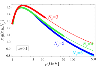
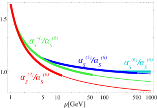
Figure 1: Schematic of a H-VFNS: PDF (left) and $\alpha_{S}$ (right) vs. $\mu$ for a selection of ${N_{F}}$ values. The preferred range of each ${N_{F}}$ branch is indicated by the thicker line. Thus, $f_{i}(x,\mu,{N_{F}}=3)$ can be used slightly above the $m_{c}$ transition, but for very large $\mu$ scales the ${N_{F}}=4,5,6$ branches are preferred as these resum the $m_{c}$ mass singularities.

The traditional VFNS introduced in the previous section can be generalized by introducing, in addition to the matching scales $\mu_{M}^{({N_{F}})}$, separate switching scales $\mu_{S}^{({N_{F}})}$. The switching scale $\mu_{S}^{({N_{F}})}$ prescribes where the transition from the scheme with ${N_{F}}$ flavors to the one with ${N_{F}}+1$ flavors is performed. Below the switching scale ($\mu<\mu_{S}^{({N_{F}})}$) physical observables are calculated in the $\mathrm{S}^{({N_{F}})}$ scheme , and above the switching scale ($\mu_{S}^{({N_{F}})}<\mu$) they are calculated in the $\mathrm{S}^{({N_{F}}+1)}$ scheme. Thus, the H-VFNS is a series of sub-schemes specified by:

$${\mathrm{S}} =\begin{cases}\mathrm{S}^{(3)};&\quad\mu\leq\mu_{S}^{(4)}\\ \mathrm{S}^{(4)};&\quad\mu_{S}^{(4)}<\mu\leq\mu_{S}^{(5)}\\ \mathrm{S}^{(5)};&\quad\mu_{S}^{(5)}<\mu\leq\mu_{S}^{(6)}\\ \mathrm{S}^{(6)};&\quad\mu_{S}^{(6)}<\mu\end{cases}$$ (2)

We refer to this scheme as the hybrid variable flavor number scheme (H-VFNS) in order to clearly distinguish it from the traditional VFNS in which the matching and the switching (transition) scales are equal. Indeed, in all practical applications to date these scales have been identified with the heavy quark masses: $\mu_{M}^{({N_{F}})}=\mu_{S}^{({N_{F}})}=m_{{N_{F}}}$; while this choice leads to considerable simplifications at the technical level, it also brings some disadvantages which we will discuss below. The theoretical basis for the implementation of the presented H-VFNS follows the general formulation of the ACOT scheme given (and proven) in Ref. Collins (1998).

The essential technical step to implement the H-VFNS is to add an explicit dependence on the number of active flavors, ${N_{F}}$, in both the PDFs $f_{a}(x,\mu,{N_{F}})$ and the strong coupling $\alpha_{S}(\mu,{N_{F}})$. This concept is illustrated notationally as:

$$f_{i}(x,\mu) \longrightarrow f_{i}(x,\mu,{N_{F}})$$

$$\alpha_{s}(\mu) \longrightarrow \alpha_{s}(\mu,{N_{F}}),$$

and we illustrate this schematically in Fig. 1 where we explicitly see the coexistence of PDFs and $\alpha_{S}$ for different $N_{F}$ values.

Instead of a single PDF, we will have a set of 4 coexisting PDFs, $f_{a}(x,\mu,N_{F})$ with $N_{F}=\{3,4,5,6\}$, that are related analytically by the $\overline{\rm MS}$ matching conditions (see Appendix A.2). Therefore, by knowing the PDFs for a specific $N_{F}$ branch, we are able to compute the related PDFs for any other number of active flavors. Likewise, we have a set of 4 coexisting strong couplings, $\alpha_{S}(\mu,N_{F})$ for $N_{F}=\{3,4,5,6\}$, that are also related analytically by the $\overline{\rm MS}$ matching conditions (see Appendix A.1).

Generating the PDFs and $\alpha_{s}$ in the H-VFNS

These PDFs and $\alpha_{s}$ are computed using the following prescription.

1. Parametrize the PDFs at a low initial scale $\mu_{0}=Q_{0}\sim 1$ GeV; as this is below the $m_{c,b,t}$ thresholds, this would correspond to $N_{F}=3$. We also choose an initial value for $\alpha_{s}(\mu_{0},N_{F}=3)$ at the same scale.

2. Starting at an initial scale $\mu_{0}$ with $N_{F}=3$, we evolve the PDFs using the DGLAP evolution equations and $\alpha_{s}(\mu,N_{F})$ with the renormalization group equations up to $\mu_{max}$. We thus obtain $f_{a}(x,\mu,N_{F}=3)$ and $\alpha_{s}(\mu,N_{F}=3)$ for scales $\mu\in[\mu_{0},\mu_{max}]$.

3. At $\mu=m_{c}$ we use the $\overline{\rm MS}$ matching conditions to compute both the $N_{F}=4$ PDFs and $\alpha_{s}$ using the $N_{F}=3$ results. We then use the $N_{F}=4$ evolution equations to obtain $f_{a}(x,\mu,N_{F}=4)$ and $\alpha_{s}(\mu,N_{F}=4)$ up to $\mu_{max}$.

4. At $\mu=m_{b}$ we again use the $\overline{\rm MS}$ matching conditions to compute both the $N_{F}=5$ PDFs and $\alpha_{s}$ using the $N_{F}=4$ results. We then use the $N_{F}=5$ evolution equations to obtain $f_{a}(x,\mu,N_{F}=5)$ and $\alpha_{s}(\mu,N_{F}=5)$ up to $\mu_{max}$.

5. At $\mu=m_{t}$ this procedure can be repeated again with $N_{F}=6$ for the top quark.

Because all the $N_{F}=\{3,4,5,6\}$ results for the PDFs $f_{a}(x,\mu,N_{F})$ and the strong coupling $\alpha_{S}(\mu,N_{F})$ are retained, the user has the freedom to choose which $N_{F}$ to use for a particular calculation. However, note that the number of active flavors used in $\alpha_{S}$ and in PDFs is always the same.

Properties of the H-VFNS

Having generated a set of $N_{F}$-dependent PDFs and strong couplings, we highlight two important properties.

1. The PDFs and strong couplings with different $N_{F}$ flavors co-exist simultaneously.

2. The PDFs and strong couplings with one $N_{F}$ value have a precise analytic relation to those with a different $N_{F}$ value which is specified by the appropriate evolution equations and the $\overline{\rm MS}$ boundary conditions at $\mu=m_{c,b,t}$ (c.f., Appendix A).

Property 1) allows us to avoid dealing with an $N_{F}$ flavor transition should it happen to lie right in the middle of a data set. For example, if we analyze the HERA $F_{2}^{charm}$ data which covers a typical range of $Q\sim[3,8]$ GeV, if we were to use the traditional VFNS then the $N_{F}$ transition between 4 and 5 flavors would lie right in the middle of the analysis region; clearly this is very inconvenient for the analysis. Because we can specify the number of active flavors $N_{F}$ in the H-VFNS, we have the option to not activate the $b$-quark in the analysis even when $\mu>m_{b}$; instead, we perform all our calculations of $F_{2}^{charm}$ using $N_{F}=4$ flavors. This will avoid any potential discontinuities in the PDFs and $\alpha_{s}$ in contrast to the traditional VFNS which forces a transition to ${N_{F}}=5$ at the $b$-quark mass.

Property 2) allows us to use the $N_{F}=4$ PDF $f_{i}(x,\mu,N_{F}=4)$ extracted from the $F_{2}^{charm}$ data set and relate this to $N_{F}=5$ and $N_{F}=6$ PDFs that can be applied at high $\mu$ scales for LHC processes. In this example note that all the HERA $F_{2}^{charm}$ data (both above and below $m_{b}$) influence the $N_{F}=5$ and $N_{F}=6$ PDFs used for the LHC processes.

Challenges Resolved

We can now see how this H-VFNS overcomes the challenges noted above. While the traditional VFNS forced the user to transition from $N_{F}=4$ to $N_{F}=5$ at $\mu=m_{b}$ (for example), because the H-VFNS approach retains the $N_{F}$ information we have the freedom to use the $N_{F}=4$ calculation for $\mu$ scales even above $m_{b}$.

The H-VFNS also shares the benefits of the FFNS in that we can avoid a $N_{F}$ transition which might lie in the middle of a data set. Furthermore, while the FFNS cannot be extended to large scales due to the uncanceled logs, the H-VFNS can be used at high scales (such as for LHC processes) because we retain the freedom to switch $N_{F}$ values and resum the additional logs where they are important.

Additionally, the H-VFNS implementation gives the user maximum flexibility in choosing where to switch between the $N_{F}$ and $N_{F}+1$ calculations. Not only can one choose different switching points for different processes (as sketched above), but we can make the switching point dependent on the kinematic variables of the process. For example, the production thresholds for charm/bottom quarks in DIS are given in terms of the photon-proton center of mass energy $W^{2}\simeq Q^{2}(1-x)/x$; thus, we could use this to define our switching scales.

An important operational question is: how far above the $\mu=m_{Q}$ can we reliably extend a particular $N_{F}$ framework. We know this will have mass singular logs of the form $\alpha_{s}\ln(\mu/m_{Q})$, so these will eventually spoil the perturbative expansion of the coefficient functions. We just need to ensure that we transition to the $N_{F}+1$ result before these logs obviate the perturbation theory. We will investigate this question numerically in Sec. V.

Relation to previous work

In closing we want to note that many of the ideas that we build upon here with the H-VFNS have been present in the literature for some time. The proof of factorization paper by Collins Collins (1998) incorporates the flexibility of introducing separate matching and switching scales, and applications to the ACOT scheme were outlined in Ref. Amundson et al. , and Ref. Thorne and Tung (2008) provides a recent review of the situation. The separate $N_{F}$ sets of the MSTW collaboration Martin et al. (2006) are precisely defined by the $\overline{\rm MS}$ matching conditions Buza et al. (1998) at ${\cal O}(\alpha_{s})$. This is extended to higher order for MSTW Martin et al. (2010) and ABKM/ABM Alekhin et al. (2010). Additionally, the NNPDF group provides PDF sets with different numbers of active flavors in Refs. Ball et al. (2011, 2013a) for NLO and NNLO. The phenomenological implications of coexisting $N_{F}$ PDF sets has been investigated in the MSTW and NNPDF frameworks Thorne (2012); Ball et al. (2013b). The extension of the ACOT scheme beyond NLO, where the PDF and $\alpha_{S}$ discontinuities appear, was presented in Ref. Stavreva et al. (2012). Putting these pieces together, and including the explicit $N_{F}$ dependence, allows us to construct a tractable implementation of the H-VFNS with user-defined switching scales.

Operationally, we are able to provide maximum flexibility with only a minimal extension of the PDF. A fully general framework as described in Ref. Amundson et al. would require a separate PDF grid (and associated evolution) for each data set with a distinct matching or switching scale. With the implementation outlined in the H-VFNS we are able to implement this economically with only three PDF grids for $N_{F}=\{3,4,5\}$; this is possible for a number of reasons as outlined below.

While we have imposed the choice $\mu_{M}^{({N_{F}})}=m_{{N_{F}}}$, we demonstrate in Appendix A.2 that when the matching conditions are implemented correctly, particularly at higher orders, the physical influence of this matching condition is minimal. On physical grounds, the natural choice for the switching scale is at or above the heavy quark mass scale $\mu_{S}^{({N_{F}})}\geq m_{{N_{F}}}$. Additionally, it is generally preferred to have the switching scale above the matching scale $\mu_{M}^{({N_{F}})}\leq\mu_{S}^{({N_{F}})}$ as this avoids the need for backward evolution. Our implementation of the H-VFNS with $m_{{N_{F}}}=\mu_{M}^{({N_{F}})}\leq\mu_{S}^{({N_{F}})}$ naturally accommodates these choices.

Therefore, our H-VFNS implementation economically requires only three PDF grids (for $N_{F}=\{3,4,5\}$), yet provides the user flexibility to use any switching scale, and the choice of the fixed matching scale $\mu_{M}^{({N_{F}})}=m_{{N_{F}}}$ has minimal impact on the physical results.

IV ${N_{F}}$ Dependence of the PDFs and $\alpha_{s}$

In this study we are using an initial PDF parameterization based on the nCTEQ “decut3” set of Ref. Kovarik et al. (2011). We use quark masses of $m_{c}=1.3$ GeV, $m_{b}=4.5$ GeV, and $m_{t}=175$ GeV, with a starting scale of $Q_{0}=1.2$ GeV which allows us to examine the charm threshold. The full set of $N_{F}=\{3,4,5,6\}$ PDFs is generated as described above using the $\overline{\rm MS}$ matching conditions applied at the quark mass values. The details of the matching are described in Appendix A.

IV.1 ${N_{F}}$ Dependence of the PDFs

We begin by illustrating the effect of the number of active flavors $N_{F}$ on the PDFs, $f_{i}(x,\mu,N_{F})$. One of the simplest quantities to examine is the momentum fraction $\left[\int_{0}^{1}x\,f_{i}(x)\,dx\right]$ carried by the PDF flavors as a function of the $\mu$-scale.

Fig. 2 shows the gluon and heavy quark momentum fractions as a function of the $\mu$ scale. For very low $\mu$ scales all the curves coincide by construction; when $\mu<m_{c,b,t}$ the charm, bottom, and top degrees of freedom will “deactivate” and the $N_{F}=4,5,6$ results will reduce to the $N_{F}=3$ result.

As we increase the $\mu$ scale, we open up new channels. For example, when $\mu>m_{c}$ the charm channel activates and the DGLAP evolution will generate a charm PDF via the $g\to c\bar{c}$ process. Because the overall momentum sum rule must be satisfied $\left[\sum_{i}\int_{0}^{1}x\,f_{i}(x)\,dx=1\right]$, as we increase the momentum carried by the charm quarks, we must decrease the momentum carried by the other partons. This interplay is evident in Fig. 2. In Fig. 2-a, we see that for $\mu=1000$ GeV, the momentum fraction of the $N_{F}=4$ gluon is decreased by $\sim 4\%$ as compared to the $N_{F}=3$ gluon. Correspondingly, in Fig. 2-b we see that at $\mu=1000$ GeV, the momentum fraction of the charm PDF is $\sim 4\%$. Thus, when we activate the charm in the DGLAP evolution, this depletes the gluon and populates the charm PDF via $g\to c\bar{c}$ process.

In a similar manner, comparing the momentum fraction of the $N_{F}=5$ gluon to the $N_{F}=4$ gluon at $\mu=1000$ GeV we see the former is decreased by $\sim 3\%$; in Fig. 2-b we see that at $\mu=1000$ GeV the momentum fraction of the bottom PDF is $\sim 3\%$.

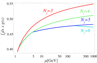
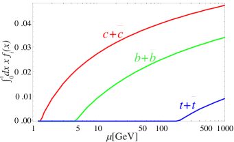
Figure 2: (a) Gluon momentum fraction; (b) Momentum fraction for $c+\bar{{c}}$, $b+\bar{{b}}$ and $t+\bar{{t}}$ quarks. The results have been obtained using NLO PDFs ($\overline{\rm MS}$) with a 2-loop $\alpha_{S}$.

The gluon PDF is primarily affected by the heavy $N_{F}$ channels as it couples via the $g\to c\bar{c},b\bar{b},t\bar{t}$ processes. The effect on the light quarks $\{u,d,s\}$ is minimal as these only couple to the heavy quarks via higher order processes ($u\bar{u}\to g\to c\bar{c}$). This property is illustrated in Fig. 3 where we display the $u$ and $\bar{u}$ quark momentum for different $N_{F}$ values. While the $N_{F}$ variation yields a $\sim 8\%$ momentum fraction shift for the gluon, the total shift of the $u$ quark is only $\sim 1\%$ of the momentum fraction.

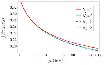
Figure 3: Momentum fraction carried by the (a) $u$-quark and (b) $\bar{u}$-quark in the 3, 4, 5, and 6 flavor schemes.

IV.2 ${N_{F}}$ Dependence of $\alpha_{s}$

The PDFs are only one piece of the full calculation; another essential ingredient is the strong coupling constant $\alpha_{S}(\mu,N_{F})$. The running coupling is sensitive to higher-order processes involving virtual quark loops; hence, it depends on the number of active quarks, and we make this dependence explicit with the $\alpha_{S}(\mu,N_{F})$ notation. More precisely, the strong coupling depends on the renormalization scale $\mu_{R}$, in contrast to the factorization scale $\mu_{F}$. However, for this work we have set $\mu_{R}=\mu_{F}=\mu$.

In Fig. 4 we display $\alpha_{S}(\mu,N_{F})$ vs. $\mu$ for different $N_{F}$ values. We choose an initial $\alpha_{S}(\mu,N_{F})$ at a low $\mu=Q_{0}$ and $N_{F}=3,$ and evolve this to larger scales using the NLO beta function. (See Appendix A.1 for details.) As we saw in Fig. 2, the $N_{F}$ transitions are evident.

There are strong constraints on $\alpha_{S}(\mu,N_{F})$ at low scales ($\mu\sim m_{\tau}$) from hadronic $\tau$ decays, and at high scales ($\mu\sim M_{Z}$) from LEP2 measurements Beringer et al. (2012); thus, it is not trivial to satisfy both limits for a fixed value of $N_{F}$.

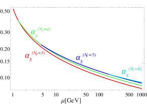
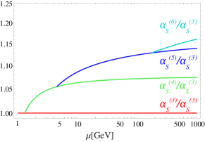
Figure 4: (a) 2-loop $\alpha_{S}$ for different number of flavors; (b) ratio of 3, 4, 5, and 6-flavor $\alpha_{S}$ to the 3-flavor one.

IV.3 Interplay between $\alpha_{S}(\mu,N_{F})$ and $g(x,\mu,N_{F})$

If we could do an all-orders calculation for any physical observable, this would be independent of $N_{F}$ and $\mu$; for finite-order calculations, any residual $\mu$ and $N_{F}$ dependence is simply an artifact of our truncated perturbation theory. Thus, the separate contributions of the perturbative QCD result must conspire to compensate the $\mu$ and $N_{F}$ dependence to the order of the calculation.

For example, when we activate the charm PDF, we find the gluon PDF is decreased. Within the limits of the perturbation theory, we would expect that the decreased contribution from the gluon initiated processes would be (at least partially) compensated by the new charm initiated processes. This compensation mechanism is clearly evident for the calculation of $F_{2}^{charm}$; additionally, we find that because the gluon initiated and charm initiated contribution generally have opposite renormalization scale dependence, the resulting VFNS prediction is more stable in $\mu$ as compared to the FFNS result Aivazis et al. (1994b).

Another compensating mechanism is evident when comparing Fig. 2 and Fig. 4 where we note that the $N_{F}$ dependence of $\alpha_{s}$ is generally opposite to that of the gluon PDF; this observation is particularly interesting as many NLO contributions are proportional to the combination $\alpha_{S}\times x\,g$. If we consider the inclusive structure functions $F_{123L}$, for example, the LO contributions are proportional to the electroweak couplings and the quark PDFs – both of which are relatively invariant under changes in $N_{F}$. Thus, the primary effect of the $N_{F}$ dependence will be to modify the NLO contributions which are dominantly proportional to $\sim\alpha_{S}\times x\,g$. For these contributions, the $x\,g$ and $\alpha_{S}$ dependence will partially cancel each other out so that the total result is relatively stable as a function of $N_{F}$ Aivazis et al. (1994b); Olness et al. (1999).

To illustrate this mechanism, we show the combination $\alpha_{S}^{(N_{R})}\times x\,g^{(N_{F})}$ vs. $x$ (in Fig. 5) and vs. $\mu$ (in Fig. 6). The compensating properties are best observed in the ratio plots (Figs. 5b and 6b).

For example, in Fig. 5b for $\mu=5$ GeV we see that if we start with $N_{F}=3$ for both $\alpha_{s}$ and $g$ (red line), the effect of changing $N_{F}=5$ for $\alpha_{s}$ increases $\alpha_{S}\times x\,g$ by 6%; but, changing $N_{F}=5$ for the gluon decreases $\alpha_{S}\times x\,g$ by roughly the same amount. Hence, the combination $\alpha_{S}\times x\,g$ is relatively stable under a change of $N_{F}$ as we see by comparing the curves labeled $\{3,3\}$ (red) and $\{5,5\}$ (cyan). This is an example of how the perturbation theory adjusts to yield a result that is (approximately) independent of $N_{F}$ at a given order of perturbation theory.

In Fig. 6 we show $\alpha_{S}\times x\,g$ vs. $\mu$ for a choice of $x$ values $\{10^{-1},10^{-3},10^{-5}\}$. While $\{3,3\}$ (red) and $\{5,5\}$ (cyan) results are roughly comparable for lower $\mu$ and higher $x$ values ($10^{-1}$), for smaller $x$ values and larger $\mu$ the shift in the gluon is not sufficient to compensate that of $\alpha_{s}$.

Reviewing Fig. 5 in more detail, we observe that the $N_{F}$ compensation works well for lower $\mu$ values $\sim(5,10)$ GeV across a broad range of $x$. For $\mu=5$ GeV, the curves labeled $\{3,3\}$ (red) and $\{5,5\}$ (cyan) match within about $\sim 2\%$ over much of the $x$ range. However, for larger $\mu=100$ GeV the compensation between ${\alpha_{S}}$ and $g$ is diminished. We will see this pattern again when we examine the physical structure functions, and this difference is driven (in part) by uncanceled mass singularities in the FFNS result.

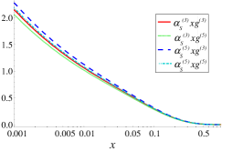
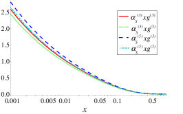
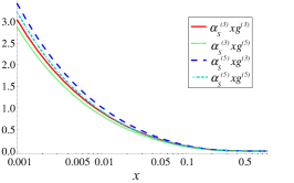
(a) Different combinations of 3- and 5-flavor ${\alpha_{S}}^{(N_{R})}xg^{(N_{F})}(x)$ as a function of $x$, for different values of $\mu$: $5$ (left), $10$ (middle) and $100$ (right) GeV.

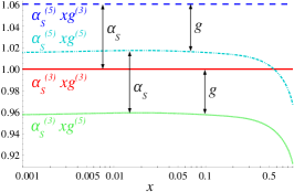
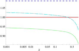
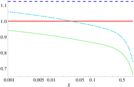
(b) Ratio of different combination of 3- and 5-flavor ${\alpha_{S}}^{(N_{R})}xg^{(N_{F})}(x)$ and ${\alpha_{S}}^{(3)}xg^{(3)}(x)$ as a function of $x$, for different values of $\mu$: $5$ (left), $10$ (middle) and $100$ (right) GeV.

Figure 5: ${\alpha_{S}}^{(N_{R})}xg^{(N_{F})}(x)$ as a function of $x$, for different values of $\mu$. The curves are labeled ${\alpha_{S}}^{(N_{R})}xg^{(N_{F})}(x)=\{N_{R},N_{F}\}$ where the first term in braces indicates the $N_{R}$ for the $\alpha_{s}$ and the second indicates the $N_{F}$ for $g$.

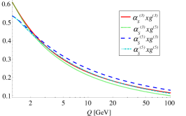
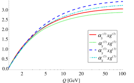
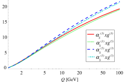
(a) Different combinations of 3- and 5-flavor ${\alpha_{S}}^{(N_{R})}xg^{(N_{F})}(x)$ as a function of $\mu$, for different values of $x$: $10^{-1}$ (left), $10^{-3}$ (middle) and $10^{-5}$ (right).

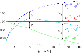
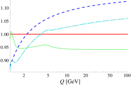
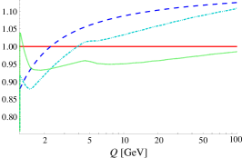
(b) Ratio of different combination of 3- and 5-flavor ${\alpha_{S}}^{(N_{R})}xg^{(N_{F})}(x)$ vs. ${\alpha_{S}}^{(3)}xg^{(3)}(x)$ as a function of $\mu$, for different values of $x$: $10^{-1}$ (left), $10^{-3}$ (middle) and $10^{-5}$ (right).

Figure 6: ${\alpha_{S}}^{(N_{R})}xg^{(N_{F})}(x)$ as a function of $\mu$, for different values of $x$. The curves are labeled ${\alpha_{S}}^{(N_{R})}g^{(N_{F})}(x)=\{N_{R},N_{F}\}$ where the first term in braces indicates the $N_{R}$ for the $\alpha_{s}$ and the second indicates the $N_{F}$ for $g$.

V Physical Structure Functions vs. ${N_{F}}$

Having examined the unphysical (but useful) combination ${\alpha_{S}}\times xg$, we now consider the physical observables $F_{2}$ and $F_{L}$ vs. $N_{F}$. In Fig. 7 we display $F_{2}$ vs. $Q$ for a choice of three $x$ values; the absolute values are shown in the upper figures, and the ratios in the lower figures. Figure 8 shows the corresponding plots for $F_{L}$. Both $F_{2}$ and $F_{L}$ were calculated at NLO and N3LO Stavreva et al. (2012) using 3 and 5 flavor H-VFNS PDFs. We observe a number of patterns in these figures.

Low $Q$: $Q<m$

At low $Q$ values, the $N_{F}=3$ and $N_{F}=5$ results coincide. This is by design as once we go below the thresholds for $N_{F}=4,5$ the charm and bottom quarks are “deactivated” and all $N_{F}$ calculations reduce to the $N_{F}=3$ result.

At low $Q$ values, we also observe there is a significant difference between the NLO and N3LO results; this difference arises from a number of sources including the fact that at low $Q$ the value of $\alpha_{s}$ is large, hence the higher order corrections are typically larger here.

High $Q$: $Q\gg m$

As we move to larger $Q$ values, we notice two distinct features.

First, at large $Q$ we find the NLO and N3LO results tend to coincide. Because $\alpha_{s}$ is decreasing at larger $Q$, the relative importance of the higher order corrections is reduced.

Second, we see that the $N_{F}=3$ and $N_{F}=5$ results slowly diverge from each other, both for the NLO and N3LO cases. This difference can be traced to the uncanceled mass singularity in the $N_{F}=3$ calculations which is roughly proportional to $\alpha_{s}\ln[Q/m]$. In the $N_{F}=5$ calculation, these logs are resummed into the heavy quark PDFs; for the $N_{F}=3$ calculation, these logs are not resummed and the calculation will be divergent in the limit $Q/m\to\infty$.

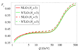
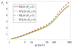
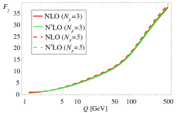
(a) Inclusive $F_{2}$ as a function of $Q$ [GeV] for different values of $x$: $10^{-1}$ (left), $10^{-3}$ (middle) and $10^{-5}$ (right).

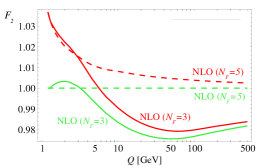
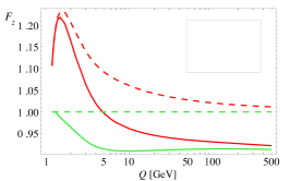
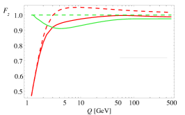
(b) Ratio of inclusive $F_{2}$ as a function of $Q$ [GeV] for different values of $x$: $10^{-1}$ (left), $10^{-3}$ (middle) and $10^{-5}$ (right).

Figure 7: Inclusive $F_{2}$ as a function of $Q$ [GeV] for different values of $x$: $10^{-1}$ (left), $10^{-3}$ (middle) and $10^{-5}$ (right). In these calculations we have chosen $\mu=Q$.

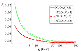
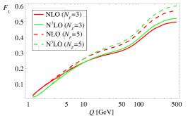
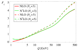
(a) Inclusive $F_{L}$ as a function of $Q$ [GeV] for different values of $x$: $10^{-1}$ (left), $10^{-3}$ (middle) and $10^{-5}$ (right).

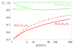
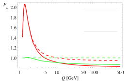
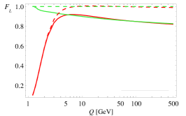
(b) Ratio of inclusive $F_{L}$ as a function of $Q$ [GeV] for different values of $x$: $10^{-1}$ (left), $10^{-3}$ (middle) and $10^{-5}$ (right).

Figure 8: Inclusive $F_{L}$ as a function of $Q$ [GeV] for different values of $x$: $10^{-1}$ (left), $10^{-3}$ (middle) and $10^{-5}$ (right). In these calculations we have chosen $\mu=Q$.

Intermediate $Q$: $Q\gtrsim m$

We now come to the critical question: how far above the charm flavor transition can we extend the $N_{F}=3$ FFNS calculation before the uncanceled logs $\alpha_{s}\ln[Q/m]$ degrade the perturbation expansion. By examining Figs. 7 and 8 we can determine the extent to which the $N_{F}=3$ and $N_{F}=5$ results diverge due to these logs. For scales $\mu=Q$ a few times the quark mass ($m_{c}$) the difference is small; but for larger scales $\mu=Q\sim 10m_{c}$ the difference can be in excess of 10% depending on the specific $x$ region. Also note, that while we are considering the inclusive $F_{2,L}$, it is only the heavy quark components which are driving the difference at large $\mu$ scales; for a less inclusive observable (such as $F_{2}^{charm}$) this effect would be even more prominent.

V.0.1 Recap

To recap, in the three kinematic regions of interest we find the following.

• In the low $Q$ region, we find the $N_{F}=3$ and $N_{F}=5$ results coincide; hence, in this region an $N_{F}=3$ FFNS result will match with any VFNS result. Thus, we can use either the $N_{F}=3$ and $N_{F}=5$ calculation in this region.

• In the region of high $Q$, we find the $N_{F}=3$ and $N_{F}=5$ results diverge logarithmically due to the uncanceled mass singularities, and in the limit $Q/m\to\infty$ the $N_{F}=3$ calculation contains divergent terms. Hence, in this region, we would expect the VFNS $N_{F}=5$ result to be most reliable.

• For $Q$ scales which are a few times the quark mass or less, the $N_{F}=3$ and $N_{F}=5$ results are comparable; for larger $Q$ scales, this difference will increase logarithmically with the scale. Thus, we can use either the $N_{F}=3$ and $N_{F}=5$ calculation in this region, but as we move to larger scales we need to transition to the $N_{F}=5$ in the VFNS.

These conclusions are illustrated in Fig. 1, and now we are able to make quantitative statements about the specific regions of validity.

In summary, the $N_{F}$ dependent PDFs provide us the freedom to choose the $N_{F}$ transitions where it is convenient for the analysis of specific data sets; however, this freedom comes with the responsibility that we must be aware of the mass singular logs and be sure not to extend a particular $N_{F}$ FFNS calculation beyond its region of reliability.

VI An Example: From Low to High Scales

We now finish with an example of how the H-VFNS scheme could be employed for a simultaneous study of both a low-scale process ($\mu\sim m_{b}$) at HERA and a high scale process ($\mu\gg m_{c,b}$) at the LHC.

At HERA, a characteristic $Q$ range for the extraction of $F_{2}^{charm}$, for example, is $\sim 2<Q<10$ GeV and this spans the kinematic region where the charm and bottom quarks become active in the PDF. These analyses can be performed using a $N_{F}=3$ FFNS calculation as the scales involved are not particularly large compared to the $m_{c,b,}$ scales. Additionally, the extraction of the $F_{2}^{charm}$ structure function is often computed using the HVQDIS program Harris and Smith (1998), and this explicitly works in a $N_{F}=3$ FFNS. This approximation is entirely adequate in this kinematic region as resummed logs are not particularly large in the relevant $Q$ region. The $F_{2}^{charm}$ structure function extracted in Aaron et al. (2011) is compared with predictions using $N_{F}=3$ FFNS PDFs from CT10f3 Lai et al. (2010) and MSTW2008f3 Martin et al. (2010) and both yield good descriptions of the data.

Conversely, at the LHC the $\mu$ range for new particle searches via the Drell-Yan process can be in excess of a TeV. For this analysis, we would want to use $N_{F}=5$ so that the charm and bottom logs are resummed.

Because the H-VFNS simultaneously provides $N_{F}=\{3,4,5,6\}$, we can analyze the HERA data in a FFNS $N_{F}=3$ context while also analyzing the LHC data in a $N_{F}=\{4,5,6\}$ VFNS context.

Operationally, we could perform a PDF fit to both a combination of HERA and LHC data by implementing the following steps.

1. Parametrize the PDFs at a low initial scale $\mu=Q_{0}\sim 1$ GeV, and generate a family of $N_{F}$ dependent PDFs as outlined in Sec. III.

2. Fit the HERA $F_{2}^{charm}$ structure function data using $N_{F}=3$ “FFNS” PDFs, $f_{i}(x,\mu,N_{F}=3)$ and $\alpha_{s}(\mu,N_{F}=3)$.

3. Fit the high-scale LHC data using $N_{F}=4,5,6$ “VFNS” PDFs, $f_{i}(x,\mu,N_{F}=4,5,6)$ and $\alpha_{s}(\mu,N_{F}=4,5,6)$.

4. Repeat steps 1) through 3) until we have a suitable minimum.

Note, because we generate all the PDFs and $\alpha_{s}$ for all $N_{F}=\{3,4,5,6\}$ flavors in step 1), the separate $N_{F}$ branches are analytically related. Furthermore, this is done using a “forward” DGLAP evolution; no “backward” DGLAP evolution is required.

Also note that because we have access to all $N_{F}=\{3,4,5,6\}$ sets, there is no difficulty in performing the HERA analysis of step 2) and the LHC analysis of step 3) in different $N_{F}$ frameworks.

Finally, as we demonstrated in Sec. V, the user is now responsible for ensuring each $N_{F}$ calculation is not used beyond its range of validity. While it is now possible to compute with $N_{F}=3$ at high $\mu$ scales, this does not necessarily give a reliable result for the cross sections.

$N_{F}$ Conversion Factors

Finally, we demonstrate how to use the family of $N_{F}$ dependent PDFs to estimate the effect of changing from $N_{F}=3$ to $N_{F}=5$ in a calculation such as the extraction of $F_{2}^{charm}$ discussed above. For example, the HVQDIS program Harris and Smith (1995, 1998) works in a $N_{F}=3$ FFNS while many of the PDFs are only available for $N_{F}=4,5$. If we have access to both $N_{F}=3$ and $N_{F}=5$ PDFs, we can simply use the correct $N_{F}$ PDF set, and the conversion between the different $N_{F}$ sets is simply given by the following identity:

$$f^{(N_{F}=5)}(x)=f^{(N_{F}=3)}(x)\left[\frac{f^{(N_{F}=5)}(x)}{f^{(N_{F}=3)}(x)}\right].$$

The term in brackets above represents the “correction factor” in converting between $N_{F}=3$ and $N_{F}=5$ PDF sets.

As we noted in Sec. IV.1, the dominant effect of changing from $N_{F}=3$ to $N_{F}=5$ was to deplete the gluon PDF which fed the charm PDF via the $g\to c\bar{c}$ process. Therefore, we can estimate this effect by comparing the shift of the gluon PDF for $N_{F}=3$ and $N_{F}=5$. This effect is shown in Fig. 9-a where we plot the gluon PDF explicitly, and in Fig. 9-b we plot the ratio. We see that even at the lowest $Q$ value displayed (10 GeV) the shift in the gluon PDF is $\sim 6\%$ and relatively insensitive to $x$, except for the highest $x$ values. Because the $x$ dependence is minimal, we can approximately extract this correction factor from the convolution of the PDFs; thus, at scales $\mu\lesssim 10$ GeV, we can estimate the effect of the $N_{F}=3$ to $N_{F}=5$ conversion by simply rescaling the gluon PDF.

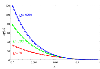
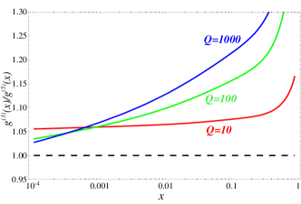
Figure 9: (a) Comparison of 3-flavor (solid lines) and 5-flavor (dashed lines) gluon for $Q=\{10,100,1000\}$ GeV; (b) ratio of 3- to 5-flavor gluon for the corresponding $Q$ values.

For example, if we are looking at charm structure functions, this is driven by the $\gamma g\to c\bar{c}$ process, plus higher order corrections. Since this process is linear in the gluon PDF, the effect would be approximately a constant overall shift; specifically, 6% for the case of $Q\sim 10$ GeV.

Even if we do not have access to both the $N_{F}=3$ and $N_{F}=5$ PDF sets, the combination $[f^{(N_{F}=5)}/f^{(N_{F}=3)}]$ is driven by the DGLAP evolution and only mildly sensitive to the detailed PDF; hence, the above technique can still provide a rough approximation as to the correction factor between the $N_{F}=3$ and $N_{F}=5$ PDFs.

VII Conclusion

We have investigated the $N_{F}$ dependence of the PDFs and proposed an extension of the traditional VFNS which we denote the H-VFNS. In this scheme, we include an explicit $N_{F}$ dependence in both the PDFs $f_{a}(x,\mu,N_{F})$ and strong coupling $\alpha_{S}(\mu,N_{F})$; this provides the user the freedom, and responsibility, to choose the appropriate $N_{F}$ values for each data set and kinematic region.

Our H-VFNS implementation economically requires only four PDF grids (for $N_{F}=\{3,4,5,6\}$), yet provides the user flexibility to use any switching scale. For a practical implementation of the H-VFNS, we choose a fixed matching scale $\mu_{M}^{({N_{F}})}=m_{{N_{F}}}$ and demonstrate that this has minimal impact on the physical results.

The H-VFNS is able to simultaneously work with low energy data (e.g., HERA data at low $Q^{2}$) in a $N_{F}=3$ FFNS framework, while also incorporating high-scale LHC data in a $N_{F}=\{3,4,5,6\}$ framework. Additionally, this can be implemented without any backward DGLAP evolution.

Although the PDFs and $\alpha_{S}(\mu,N_{F})$ are discontinuous across flavor thresholds at higher orders, the H-VFNS provides the user the flexibility to shift the $N_{F}$ transition for individual data sets and kinematic regions to avoid complications.

Thus, the H-VFNS provides a valuable tool for fitting data across a wide variety of processes and energy scales from low to high.

Appendix A Evolution and Matching Conditions

A.1 ${\alpha_{S}}$ Evolution & Matching Conditions

The running of the ${\alpha_{S}}(\mu,N_{F})$ is given by the renormalization group equation:

$$\mu^{2}\frac{d\alpha_{s}}{d\mu^{2}}=\beta(\alpha_{s})=-\left(b_{0}\alpha_{s}^{2}+b_{1}\alpha_{s}^{3}+b_{2}\alpha_{s}^{4}+...\right).$$

At the NLO (2-loop) level, which we use in this work, we obtain

$${\alpha_{S}}(\mu^{2},N_{F}) = \frac{1}{b_{0}\ln\frac{\mu^{2}}{\Lambda^{2}}}\left(1-\frac{b_{1}}{b_{0}^{2}}\frac{\ln\left(\ln\mbox{$\frac{\mu^{2}}{\Lambda^{2}}$}\right)}{\ln\mbox{$\frac{\mu^{2}}{\Lambda^{2}}$}}\right),$$

where $b_{0}=(33-2N_{F})/12\pi$ and $b_{1}=(153-19N_{F})/24\pi^{2}$. The $N_{F}$ dependence arises from the virtual quark loops which enter at higher orders.

The relation of $\alpha_{s}$ across flavor thresholds for $N_{F}$ and $N_{F}+1$ flavors is computed to be Beringer et al. (2012):

$$\alpha_{S}(\mu^{2},N_{F+1}) = \alpha_{S}(\mu^{2},N_{F})\,\biggl{[}1+$$

$$\left.\sum_{k=1}^{\infty}\sum_{\ell=0}^{k}\,c_{k\ell}\,\left[\alpha_{S}(\mu^{2},N_{F})\right]^{k}\,\ln^{l}\left(\frac{\mu^{2}}{m^{2}}\right)\right],$$

where $c_{10}=0$ and $c_{20}=-11/72\pi^{2}$. Thus, even if we perform the matching at $\mu=m$ we find

$$\alpha_{S}(m^{2},N_{F}+1)=\alpha_{S}(m^{2},N_{F})\,+c_{20}\alpha_{S}^{3}(m^{2},N_{F})$$

such that there is a ${\cal O}\left(\alpha_{S}^{3}\right)$ discontinuity in $\alpha_{S}$.

In the above, the $\mu$ scale appearing in the argument of $\alpha_{S}$ is more precisely the renormalization scale $\mu_{R}$; this is distinguished from the factorization scale $\mu_{F}$ appearing in the argument of PDF. However, in this work, we choose to set $\mu_{R}=\mu_{F}=\mu$.

Note also that there are in fact two versions of the FFNS scheme, which are characterized by different treatment of the number of active flavors entering ${\alpha_{S}}$ (denoted here as $N_{R}$, to be distinguished from the number of flavors entering PDF evolution $N_{F}$). In the “classical” FFNS, $N_{R}=N_{F}$. In the modified version, $N_{R}$ is incremented across flavor thresholds as in the VFNS while $N_{F}$ remains fixed. Discussion of advantages and disadvantages of these two formulations of FFNS can be found in Martin et al. (2006); Gluck and Reya (2007). In particular, allowing $N_{R}$ to vary can help the running ${\alpha_{S}}$ accommodate experimental constraints from both high ($\sim M_{Z}$) and low ($\sim m_{\tau}$) scales Beringer et al. (2012); Berger et al. (2010).

A.2 PDF Evolution & Matching Conditions

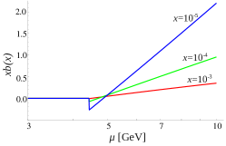
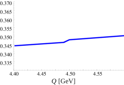
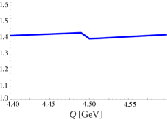
Figure 10: a) Discontinuity in the $b$-quark PDF $f_{b}(x,\mu)$ at NNLO vs. $\mu$ for $x$={$10^{-3},10^{-4},10^{-5}\}$. b) & c) Discontinuity for $F_{L}$ vs. $Q$ for $x$={$10^{-3},10^{-5}\}$ (left to right) at NNLO in the region of the bottom mass, $m_{b}=4.5$ GeV as computed in Ref. Stavreva et al. (2012).

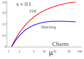
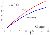
(a) Comparison of charm NLO matching and DGLAP PDFs for two choices of $x$.

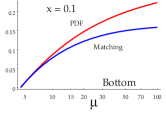
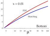
(b) Comparison of bottom NLO matching and DGLAP PDFs for two choices of $x$.

Figure 11: Comparison of charm and bottom matching conditions at NLO with the DGLAP evolved PDFs for $x=\{0.1,0.01\}$.

The relation of the PDFs with $N_{F}+1$ flavors to that of $N_{F}$ can be computed perturbatively Buza et al. (1996, 1998). The explicit form of these matching conditions can be found e.g. in eqs. (2.37)-(2.41) and Appendix B of Ref. Buza et al. (1998). For the purpose of further discussion we show here only a symbolic form of the matching conditions

$$\tilde{f}_{i}(x,\mu,N_{F}+1)=A^{ij}\otimes\,\tilde{f}_{j}(x,\mu,N_{F}),\\$$ (4)

where

$$\begin{split}A^{ij}&=\delta^{ij}+\frac{{\alpha_{S}}}{2\pi}\left(a_{1}^{ij}+b_{1}^{ij}\,\ln\left[\frac{\mu^{2}}{m^{2}}\right]\right)\\ &\quad+\left(\frac{{\alpha_{S}}}{2\pi}\right)^{2}\,\left(a_{2}^{ij}+b_{2}^{ij}\,\ln\left[\frac{\mu^{2}}{m^{2}}\right]+c_{2}^{ij}\,\ln^{2}\left[\frac{\mu^{2}}{m^{2}}\right]\right)+...\end{split}$$ (5)

In the above equation $\tilde{f}_{i}$ can be a combination of light parton densities ($f_{i}+f_{\bar{i}}$), heavy parton densities ($f_{H}+f_{\bar{H}}$), the singlet combination of parton densities $\Sigma$, or the gluon. Note that there is an implicit summation over the above combinations. Coefficients $a^{ij}$, $b^{ij}$, $\cdots$ can be computed perturbatively. While we have not indicated it explicitly, all quantities on the RHS of Eq. (4) (including $\alpha_{S}(N_{F})$) are evaluated with $N_{F}$ flavors, and those on the LHS are evaluated with $N_{F}+1$ flavors.

Note that the QCDNUM Botje (2011) program includes the NNLO evolution with the discontinous and NNLO matching conditions.

In the $\overline{\rm MS}$ scheme the $a_{1}^{ij}$ term is computed to be zero, while the $a_{2}^{ij}$ term is non-zero. Because $a_{1}^{ij}=0$, if we perform the matching between $N_{F}$ and $N_{F}+1$ flavors at $\mu=m$, the $\ln(\mu/m)$ terms vanish and we find at NLO [${\cal O}({\alpha_{S}}^{1})$] that $f_{i}(x,\mu=m,N_{F}+1)=f_{i}(x,\mu=m,N_{F})$; that is, the PDFs are continuous. This is why, at NLO, the VFNS implemented the matching automatically at $\mu=m$. Because $a_{2}^{ij}\not=0$, at NNLO and beyond the PDFs will acquire discontinuities of ${\cal O}({\alpha_{S}}^{2})$; therefore, there is no longer any special benefit obtained by forcing the $N_{F}$ transition at $\mu=m$.

For example, the discontinuity of the $b$-quark PDF is shown in Fig. 10-a, and curiously this yields a slightly negative value just above the transition point for $f_{b}(x,\mu\gtrsim m,N_{F}=5)$. There is a corresponding discontinuity in the gluon PDF (not shown) which has a positive shift, as it must to ensure the PDF sum rules are satisfied.

These discontinuities exhibit themselves in the physical observables such as the structure functions as shown in Fig. 10-b and Fig. 10-c. These discontinuities are formally higher order, and will be reduced order by order as we extend the perturbation theory. It is interesting to note that $F_{L}$ for the larger $x$ value ($10^{-3}$) has a slightly positive discontinuity while at the smaller $x$ value ($10^{-5}$) the discontinuity is negative. This reflects the shift between the (positive) gluon and the (negative) quark contributions in the different $x$ regions. It is this mixture of the gluon and the quark terms which will ensure the physical observable is continuous up to the specified order of perturbation theory, while the PDF will always remain discontinuous at ${\cal O}({\alpha_{S}}^{2})$.

In the presented H-VFNS, we choose to compute the matching between $N_{F}$ and $N_{F}+1$ flavors at $\mu=m$ (because the logs vanish); however, since we retain both the $N_{F}$ and $N_{F}+1$ PDFs for $\mu\geq m$, the user has the choice to compute in either the $N_{F}$ or $N_{F}+1$ framework, whichever is more suitable. Because the traditional VFNS did not provide PDFs for $N_{F}$ flavors at $\mu\geq m$, this was previously not an option.

The matching conditions of Eqs. (4) and (5) essentially represent a perturbative expansion of the DGLAP evolution equations, up to an additional constant term $a_{k}^{ij}$.

We observe that if we choose to perform the matching not at $\mu=m$ but instead at a higher scale such as $\mu=2m$, the PDF boundary condition for the heavy quark is not $f_{c}(x,\mu,N_{F}=4)=0$. Instead, the correct condition at NLO is:

$$f_{c}(x,\mu,N_{F} = 4)\simeq 0+\frac{{\alpha_{S}}(\mu,N_{F}=3)}{2\pi}\,\ln\left[\frac{\mu^{2}}{m_{c}^{2}}\right]\,\times$$ (6)

$$\times\quad P_{qg}\otimes g(x,\mu,N_{F}=3)+...$$

Note, the LHS uses $N_{F}=4$ PDFs and the RHS uses $N_{F}=3$ PDFs.

These matching conditions are displayed in Fig. 11 where we compare these to the DGLAP evolved PDF distribution at NLO. We see for scales near the matching point $\mu\sim m$, the differences are small. However, if the matching is performed away from the $\mu\sim m$ region, then the differences are larger. This is because the matching of Eq. (6) is only computed to NLO, so it only includes a single partonic splitting, while the DGLAP evolution resums an infinite tower of partonic emissions. The difference comes from the missing second-order splittings which are proportional to ${\alpha_{S}}^{2}\,\ln(\mu/m)$. If we repeat this exercise and compute the matching to NNLO, then we will include the ${\alpha_{S}}^{2}\,\ln(\mu/m)$ contributions, but miss the ${\alpha_{S}}^{3}\,\ln(\mu/m)$. Thus the curves in Fig. 11 will remain comparable for a larger range of $\mu\gtrsim m$.

In this analysis, our matching scale is always taken to be the quark mass, $\mu_{M}^{({N_{F}})}=m_{{N_{F}}}$. This provides us the benefit that the PDF with ${N_{F}}$ active flavors is defined for all values above $\mu=m_{{N_{F}}}$ without invoking backward-evolution.

In the traditional VFNS, the switching scale $\mu_{S}^{({N_{F}})}$ was forced to be equal to the matching scale, which was set to the quark masses: $\mu_{S}^{({N_{F}})}=\mu_{M}^{({N_{F}})}=m_{{N_{F}}}$. For the H-VFNS, the switching scale $\mu_{S}^{({N_{F}})}$ is not predefined by the PDF set but can freely be chosen by the user.

The resulting PDFs will, to some extent, depend on the matching scale $\mu_{M}^{({N_{F}})}$, but as Fig. 11 demonstrates this effect will be insignificant so long as $\mu_{M}^{({N_{F}})}\sim m_{{N_{F}}}$. Likewise, resulting observables will, to some extent, depend on the switching scale $\mu_{S}^{({N_{F}})}$, but as Figs. 7 and 8 demonstrate this effect will be insignificant so long as we do stay within the region of validity.

References

- Lai et al. (2010) H.-L. Lai, M. Guzzi, J. Huston, Z. Li, P. M. Nadolsky, et al., Phys.Rev. D82, 074024 (2010), eprint 1007.2241.
- Gao et al. (2013) J. Gao, M. Guzzi, J. Huston, H.-L. Lai, Z. Li, et al. (2013), eprint 1302.6246.
- Schienbein et al. (2008) I. Schienbein et al., Phys. Rev. D77, 054013 (2008), eprint 0710.4897.
- Schienbein et al. (2009) I. Schienbein, J. Yu, K. Kovarik, C. Keppel, J. Morfin, et al., Phys.Rev. D80, 094004 (2009), eprint 0907.2357.
- Aivazis et al. (1994a) M. A. G. Aivazis, F. I. Olness, and W.-K. Tung, Phys. Rev. D50, 3085 (1994a), eprint hep-ph/9312318.
- Aivazis et al. (1994b) M. Aivazis, J. C. Collins, F. I. Olness, and W.-K. Tung, Phys.Rev. D50, 3102 (1994b), eprint hep-ph/9312319.
- Kramer et al. (2000) M. Kramer, F. I. Olness, and D. E. Soper, Phys.Rev. D62, 096007 (2000), eprint hep-ph/0003035.
- Tung et al. (2002) W.-K. Tung, S. Kretzer, and C. Schmidt, J.Phys. G28, 983 (2002), eprint hep-ph/0110247.
- Kretzer and Schienbein (1998) S. Kretzer and I. Schienbein, Phys.Rev. D58, 094035 (1998), eprint hep-ph/9805233.
- Guzzi et al. (2012) M. Guzzi, P. M. Nadolsky, H.-L. Lai, and C.-P. Yuan, Phys.Rev. D86, 053005 (2012), eprint 1108.5112.
- Stavreva et al. (2012) T. Stavreva, F. Olness, I. Schienbein, T. Jezo, A. Kusina, et al., Phys.Rev. D85, 114014 (2012), eprint 1203.0282.
- Kotko and Slominski (2012a) P. Kotko and W. Slominski, Phys.Rev. D86, 094008 (2012a), eprint 1206.4024.
- Kotko and Slominski (2012b) P. Kotko and W. Slominski, pp. 819–822 (2012b), eprint 1206.3517.
- Kniehl et al. (2011) B. Kniehl, G. Kramer, I. Schienbein, and H. Spiesberger, Phys.Rev. D84, 094026 (2011), eprint 1109.2472.
- Martin et al. (2009) A. D. Martin, W. J. Stirling, R. S. Thorne, and G. Watt, Eur. Phys. J. C63, 189 (2009), eprint 0901.0002.
- Thorne and Roberts (1998) R. S. Thorne and R. G. Roberts, Phys. Rev. D57, 6871 (1998), eprint hep-ph/9709442.
- Thorne (2006) R. Thorne, Phys.Rev. D73, 054019 (2006), eprint hep-ph/0601245.
- Cacciari et al. (1998) M. Cacciari, M. Greco, and P. Nason, JHEP 9805, 007 (1998), eprint hep-ph/9803400.
- Forte et al. (2010) S. Forte, E. Laenen, P. Nason, and J. Rojo, Nucl.Phys. B834, 116 (2010), eprint 1001.2312.
- Ball et al. (2011) R. D. Ball, V. Bertone, F. Cerutti, L. Del Debbio, S. Forte, et al., Nucl.Phys. B849, 296 (2011), eprint 1101.1300.
- Ball et al. (2013a) R. D. Ball, V. Bertone, S. Carrazza, C. S. Deans, L. Del Debbio, et al., Nucl.Phys. B867, 244 (2013a), eprint 1207.1303.
- Alekhin et al. (2010) S. Alekhin, J. Blumlein, S. Klein, and S. Moch, Phys.Rev. D81, 014032 (2010), eprint 0908.2766.
- Alekhin et al. (2012) S. Alekhin, J. Blumlein, and S. Moch, Phys.Rev. D86, 054009 (2012), eprint 1202.2281.
- Gluck et al. (2008a) M. Gluck, P. Jimenez-Delgado, and E. Reya, Eur.Phys.J. C53, 355 (2008a), eprint 0709.0614.
- Jimenez-Delgado and Reya (2009a) P. Jimenez-Delgado and E. Reya, Phys. Rev. D79, 074023 (2009a), eprint 0810.4274.
- Gluck et al. (2008b) M. Gluck, P. Jimenez-Delgado, E. Reya, and C. Schuck, Phys.Lett. B664, 133 (2008b), eprint 0801.3618.
- Jimenez-Delgado and Reya (2009b) P. Jimenez-Delgado and E. Reya, Phys. Rev. D80, 114011 (2009b), eprint 0909.1711.
- Thorne and Tung (2008) R. Thorne and W. Tung (2008), eprint 0809.0714.
- Olness and Schienbein (2009) F. Olness and I. Schienbein, Nucl.Phys.Proc.Suppl. 191, 44 (2009), eprint 0812.3371.
- Andersen et al. (2010) J. Andersen et al. (SM and NLO Multileg Working Group), pp. 21–189 (2010), eprint 1003.1241.
- Collins (1998) J. C. Collins, Phys.Rev. D58, 094002 (1998), eprint hep-ph/9806259.
- (32) J. Amundson, F. I. Olness, C. Schmidt, W. Tung, and X. Wang, Theoretical description of heavy quark production in DIS (1998), http://lss.fnal.gov/archive/1998/conf/Conf-98-153-T.pdf.
- Collins and Tung (1986) J. C. Collins and W.-K. Tung, Nucl.Phys. B278, 934 (1986).
- Olness and Scalise (1998) F. I. Olness and R. J. Scalise, Phys.Rev. D57, 241 (1998), eprint hep-ph/9707459.
- Nadolsky and Tung (2009) P. M. Nadolsky and W.-K. Tung, Phys.Rev. D79, 113014 (2009), eprint 0903.2667.
- Olness et al. (1999) F. I. Olness, R. Scalise, and W.-K. Tung, Phys.Rev. D59, 014506 (1999), eprint hep-ph/9712494.
- Kniehl et al. (2005a) B. Kniehl, G. Kramer, I. Schienbein, and H. Spiesberger, Phys.Rev. D71, 014018 (2005a), eprint hep-ph/0410289.
- Kniehl et al. (2005b) B. Kniehl, G. Kramer, I. Schienbein, and H. Spiesberger, Eur.Phys.J. C41, 199 (2005b), eprint hep-ph/0502194.
- Kniehl et al. (2008) B. A. Kniehl, G. Kramer, I. Schienbein, and H. Spiesberger, Phys.Rev. D77, 014011 (2008), eprint 0705.4392.
- Lai et al. (2000) H. Lai et al. (CTEQ Collaboration), Eur.Phys.J. C12, 375 (2000), eprint hep-ph/9903282.
- Martin et al. (2006) A. Martin, W. Stirling, and R. Thorne, Phys.Lett. B636, 259 (2006), eprint hep-ph/0603143.
- Martin et al. (2010) A. Martin, W. Stirling, R. Thorne, and G. Watt, Eur.Phys.J. C70, 51 (2010), eprint 1007.2624.
- Beringer et al. (2012) J. Beringer et al. (Particle Data Group), Phys.Rev. D86, 010001 (2012).
- Aktas et al. (2006) A. Aktas et al. (H1 Collaboration), Eur.Phys.J. C45, 23 (2006), eprint hep-ex/0507081.
- Botje (2011) M. Botje, Comput. Phys. Commun. 182, 490 (2011), eprint 1005.1481.
- Buza et al. (1998) M. Buza, Y. Matiounine, J. Smith, and W. van Neerven, Eur.Phys.J. C1, 301 (1998), eprint hep-ph/9612398.
- Thorne (2012) R. Thorne, Phys.Rev. D86, 074017 (2012), eprint 1201.6180.
- Ball et al. (2013b) R. D. Ball et al. (The NNPDF Collaboration), Phys.Lett. B723, 330 (2013b), eprint 1303.1189.
- Kovarik et al. (2011) K. Kovarik, I. Schienbein, F. Olness, J. Yu, C. Keppel, et al., Phys.Rev.Lett. 106, 122301 (2011), eprint 1012.0286.
- Aaron et al. (2011) F. Aaron et al. (H1 Collaboration), Eur.Phys.J. C71, 1769 (2011), eprint 1106.1028.
- ATLAS Collaboration (2013) ATLAS Collaboration, ATLAS-CONF-2013-017 (2013).
- Chatrchyan et al. (2013) S. Chatrchyan et al. (CMS Collaboration) (2013), eprint 1302.4794.
- Harris and Smith (1998) B. Harris and J. Smith, Phys.Rev. D57, 2806 (1998), eprint hep-ph/9706334.
- Harris and Smith (1995) B. Harris and J. Smith, Nucl.Phys. B452, 109 (1995), eprint hep-ph/9503484.
- Gluck and Reya (2007) M. Gluck and E. Reya, Mod.Phys.Lett. A22, 351 (2007), eprint hep-ph/0608276.
- Berger et al. (2010) E. L. Berger, M. Guzzi, H.-L. Lai, P. M. Nadolsky, and F. I. Olness, Phys.Rev. D82, 114023 (2010), eprint 1010.4315.
- Buza et al. (1996) M. Buza, Y. Matiounine, J. Smith, R. Migneron, and W. van Neerven, Nucl.Phys. B472, 611 (1996), eprint hep-ph/9601302.