A note on Keen’s model: The limits of Schumpeter’s “Creative Destruction”

Abstract

This paper presents a general solution for a recent model by Keen for endogenous money creation. The solution provides an analytic framework that explains all significant dynamical features of Keen’s model and their parametric dependence, including an exact result for both the period and subsidence rate of the Great Moderation. It emerges that Keen’s model has just two possible long term solutions: stable growth or terminal collapse. While collapse can come about immediately from economies that are nonviable by virtue of unsuitable parameters or initial conditions, in general the collapse is preceded by an interval of exponential growth. In first approximation, the duration of that exponential growth is half a period of a sinusoidal oscillation. The period is determined by reciprocal of the imaginary part of one root of a certain quintic polynomial. The real part of the same root determines the rate of growth of the economy. The coefficients of that polynomial depend in a complicated way upon the numerous parameters in the problem and so, therefore, the pattern of roots. For a favorable choice of parameters, the salient root is purely real. This is the circumstance that admits the second possible long term solution, that of indefinite stable growth, i.e. an infinite period.

Keywords: Keen model, Financial instability hypothesis, Asymptotic solution, Nonlinear dynamics, Endogenous money

JEL: B50, C62, C63, E12, E47

1 Introduction

In Keen (1995), Keen (2011b), Keen (2011c), Keen (2012), Steve Keen has introduced a mathematical formalism that addresses the Financial Instability Hypothesis of Minsky (2008) in the form of low order nonlinear systems of differential equations. When parameters are set to values consistent with estimates from macroeconomic modeling, models of this kind developed by Keen can exhibit instability reminiscent of that studied in chaos theory and, more important, instability much like that seen in the Great Moderation followed by the rapid economic spiral downward commencing in 2008.

Nonlinear systems often have a rich spectrum of behaviors as the governing parameters are changed and here, where there are ten or more parameters, exploring all possible such behaviors would appear a daunting task, although perhaps not hopelessly so in that models relevant to the real world occupy only a modest range of the otherwise mathematically unbounded parameter space. One way to classify such systems is to ask for a given set of parameters what are the possible long time characteristic (“asymptotic”) behaviors of the system for a wide range of initial conditions (though here, too, considering only “realistic”, rather than all possible, initial conditions).

To speak now of the specific model explored here, one such behavior is that noted; collapse in the long term, with various economic quantities decaying exponentially with time. It is significant that this collapse is always a possible terminal solution, regardless of parameter settings. Nonetheless, this collapse is not always the invariable long time characteristic behavior for all initial conditions of interest. Rather, for only certain parameter regimes does one realize this limit irrespective of initial conditions. For other parameter regimes, this collapse can only come about for an exceedingly small range of possible starting conditions and quite another long term solution is the tendency approached under most economic conditions: a stable, steadily growing, “Schumpeter economy” as Keen has termed this model.

Though Keen’s model is an intricate ninth order nonlinear system, quite remarkably it admits a general asymptotic solution — that is, one with nine free parameters — whose form depends upon particular roots that emerge from solving an ordered sequence of algebraic equations with coefficients depending on both model parameters and previous roots in the sequence. Briefly one finds first a quintic, as derived in the main body of the paper. If the root with largest real part is real, the solution is stable, if a complex pair, unstable. That root enters into coefficients of the next polynomial, of seventh degree. Its derivation is more involved and hence confined to an appendix. A complex root pair of that polynomial explains the Great Moderation of Keen’s model. Derivation of a final polynomial depending on all the preceding is briefly sketched. In total nine unique exponents result, which can be thought of as a nonlinear basis set much as Cvitanović (1992) speaks of zeta functions as the nonlinear equivalent of a Fourier transform.

Existence of such an asymptotic solution (that it has a finite spanning basis set of exponents) shows that long term trajectories are not chaotic but rather entirely deterministic. The only uncertainty in the solution arises instead in the preliminary adjustment phase, of about a decade, where model conditions in the initial nine-dimensional parameter space collapse onto a lower dimensional attractor. And even this latter uncertainty is in principle amenable to resolution, requiring approximation of the associated projection operator.

This study aims to identify those parameters in an economy that play the greatest role in precipitating the endogenous instability that Minsky so presciently foresaw or, alternately expressed, those parameters that, if altered, could most easily mitigate the potential for instability. A careful delineation of the sensitivity of this economic model to the various governing parameters reveals that just a few are key. The most critical are capital-output ratio, the return to capital, and the interest rate.

From the standpoint of policy, the capital-output ratio is an economic factor hardly amenable to intervention in any practical way, but rather reflects the complex interaction of diverse factors such as the overall degree and nature of industrialization, of technological adoption, of financialization of the economy, and so on. But the return to capital is more immediately affected by, among other things, tax policy and the bargaining power (or lack thereof) of unions, and the interest rate is of course a direct function of monetary policy.

However the model explored in this first work is confined to investment, the debt service for which is paid from the revenue stream generated by the capital asset. Far more damaging is what Minsky identified as the inevitable secular trend in good economic times towards increased “Ponzi finance,” where investment in already existing assets fuels a bubble, and debt service requires either further borrowing or else sell-off of the asset in a (hoped for) rising market. Work that explores the latter direction is reported in the very recent paper of Grasselli and Costa Lima (2012), who determine equilibria and the local stability of both a third-order model by Keen and then the authors’ extension to a fourth-order system, which incorporates dynamical evolution of Ponzi finance through the economic cycle. A key finding is that Ponzi financing destabilizes what were otherwise stable equilibria of the system.

2 Model Introduction

The model considered here is a system taken from Keen (2011a), but see also the detailed discussion and development of essentially the same model in Keen (2012):

$$\frac{dB_{C}}{dt} = \frac{F_{L}}{\tau_{RL}(\pi_{r})}-\frac{B_{C}}{\tau_{LC}(\pi_{r})}$$ (1)

$$\frac{dB_{PL}}{dt} = r_{L}\,F_{L}-r_{D}\,F_{D}-r_{D}\,W_{D}-\frac{B_{PL}}{\tau_{B}}$$ (2)

$$\frac{dF_{L}}{dt} = \frac{B_{C}}{\tau_{LC}(\pi_{r})}-\frac{F_{L}}{\tau_{RL}(\pi_{r})}+P_{C}\,Y_{r}\,Inv(\pi_{r})$$ (3)

$$\frac{dF_{D}}{dt} = r_{D}\,F_{D}-r_{L}\,F_{L}+\frac{B_{C}}{\tau_{LC}(\pi_{r})}-\frac{F_{L}}{\tau_{RL}(\pi_{r})}+\frac{B_{PL}}{\tau_{B}}+\frac{W_{D}}{\tau_{W}}-\frac{Y_{r}\,W}{a(t)}+P_{C}\,Y_{r}\,Inv(\pi_{r})$$ (4)

$$\frac{dW}{dt} = \left(Ph(\lambda)+\omega\,(g(\pi_{r})-(\alpha+\beta))-\frac{1}{\tau_{Pc}}\,\left(1-\frac{W}{a(t)\,(1-s)\,P_{C}}\right)\right)\,W$$ (5)

$$\frac{dP_{C}}{dt} = -\frac{1}{\tau_{Pc}}\,\left(P_{C}-\frac{W}{a(t)\,(1-s)}\right)$$ (6)

$$\frac{dK_{r}}{dt} = g(\pi_{r})\,K_{r}$$ (7)

$$\frac{d\lambda}{dt} = (g(\pi_{r})-(\alpha+\beta))\,\lambda$$ (8)

where $a(t)=a_{0}\,\exp(\alpha\,t)$ models the growth of productivity over time. Population growth is modeled as $N_{0}\exp(\beta\,t)$ (the effect of which is incorporated implicitly in the system above via the growth rate $\beta$, in contrast to the explicit dependence on $a(t)$). The rate of profit is

$$\pi_{r}=\frac{1}{v\,P_{C}\,Y_{r}}\,\left(P_{C}\,Y_{r}-W\,Y_{r}/a(t)-\left(r_{L}\,F_{L}-r_{D}\,F_{D}\right)\right)\,.$$ (9)

We relate capital to output via $Y_{r}=K_{r}/v$. The rate of economic growth is given by $g=Inv(\pi_{r})/v-\delta$. Auxiliary functions defined in terms of a generalized exponential are

$$Inv(\pi_{r}) = G(\pi_{r},1/25,1/25,2,0)$$

$$Ph(\lambda) = G(\lambda,96/100,0,2,-1/25)$$

$$\tau_{RL}(\pi_{r}) = G(\pi_{r},3/100,10,100,3)$$

$$\tau_{LC}(\pi_{r}) = G(\pi_{r},3/100,2,-50,1/2)$$

where

$$G(x,x_{\nu},y_{\nu},s,m)=(y_{\nu}-m)\,\exp\left(s\,\left(x-x_{\nu}\right)/\left(y_{\nu}-m\right)\right)+m\,.$$

This system differs from Keen only in that the evolution equation for worker deposits, $W_{D}$, has been eliminated since, by an accounting identity, the sum of $W_{D}(t)+F_{D}(t)+B_{PL}(t)-F_{L}(t)\equiv cst$ is invariant in time and so $W_{D}$ can be always computed in terms of the remaining variables. Values for the parameters are chosen as stated in Table 1 and initial conditions in Table 2. The latter are supplemented with $W_{D}(0)=13$ and hence $cst=12$.

Table 1: Standard parameters for the model specified in (1 - 8)

$\alpha=0.015$	$\beta=0.02$	$\delta=0.01$	$\omega=0.1$
$\tau_{B}=1$	$\tau_{W}=1/26$	$\tau_{Pc}=1$	$s=0.27$
$a_{0}=1$	$v=3$	$r_{L}=0.05$	$r_{D}=0.01$

Table 2: Initial conditions for (1 - 8)

$B_{C}(0)=12$	$B_{PL}(0)=5$	$F_{L}(0)=100$	$F_{D}(0)=70$
$W(0)=1$	$P_{C}(0)=1$	$K_{r}(0)=900$	$\lambda(0)=1$

Briefly, $B_{C}$ is bank capital, $B_{PL}$ the flow of funds in and out of the bank in e.g., interest payments on deposits and loans, $F_{L}$ monies borrowed by a firm for investment, $F_{D}$ firm deposits at the bank, $W$ wages paid to workers, $P_{C}$ the price of goods, $K_{r}$ capital, and $\lambda$ the employment rate. A block “Phillips” diagram that represents the interaction of these variables is shown in Figure 1.

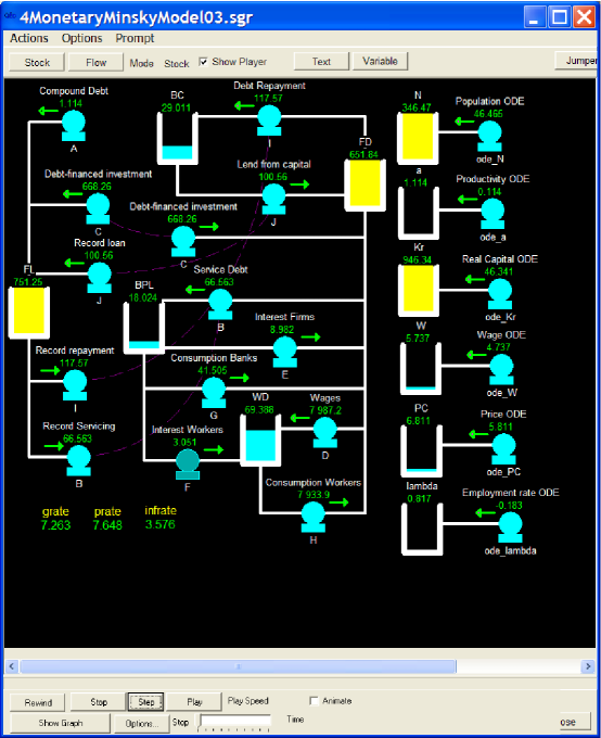
Figure 1: A Phillips diagram of (1 – 8) prepared using the QED software package developed by an anonymous collaborator of Steve Keen.

The central assumption of the model is the apostate view of Schumpeter (1934) on endogenous expansion of credit money by the banking system. As noted in Fontana (2000), the modern monetary theory of production has two branches; the Circuitist school — reflected in this model in the specific appeal to the three agent model of Graziani (1990): a buyer, a seller, and a bank — and the post-Keynesian school. The focus of the latter on liquidity preference arising from the zero elasticity of production and substitution of money is not part of the model but one can imagine various means of its incorporation. Moreover the model is about the growth of credit money, not fiat money of a sovereign government per se, although the existence of the latter is implicit in the tacit acceptance of currency itself. But here, too, a suitable generalization is readily envisioned, with the central distinction contra Graziani, of the asymmetry of only two agents — government and non-government — giving rise to the point first noted by Lerner (1970) of the irrelevance of government “debt”. The model is about the dynamics of debt, whose salience at the present time is apparent. Precisely because of the ubiquity of instability, perhaps the most interesting direction in which one might extend the model would be to include a significant role for equity-based, rather than debt-based, financing, the stabilizing influence of which has long been argued by Michael Hudson.

Perhaps the most important addition to Keen’s model in light of the post-industrial financialization of the economy would be a store of value modeled by a lumped parameter asset proxy representing equities and real estate, introducing the competitive relation between asset pricing and commodity and wage pricing.

Other significant features include increased (“speculative”) borrowing over and above profits by firms during booms and diminished (“hedge”) borrowing below the prevailing profit level during slumps, and upward wage pressure in a tight labor market. Note finally that in this simple model there are no explicit fixed (depreciating) capital assets, only deposits. And workers live always within their means; they do not take out loans.

While greatly simplified in many respects, Keen’s model is nonetheless an extremely valuable paradigm for understanding endogenous money creation as well as the intrinsic instability of a debt-based economy. This is all the more so true given that, as this paper demonstrates, one can completely characterize all the essential dynamics in analytic terms and hence dissect all the parametric dependences of the model with no need of time stepping numerous particular cases, looking for common patterns by heuristic means.

3 Analysis

Initially there are eight unknowns governed by eight equations; the coefficients of the functions

$$[B_{C},B_{PL},F_{L},F_{D},W,P_{C},K_{r},\lambda]\,.$$

As noted, we eliminate $W_{D}$ from the identity that $F_{L}-F_{D}-B_{PL}-W_{D}$ is constant. The value of this initial constant is subdominant relative to assumed exponentially growing solutions and so is dropped from the system, that is, the so-called “leading order” balance imposes that the four exponential terms sum to zero. Absent that initial constant, the resulting system is homogeneous in the unknowns. To fix a solution of this nonlinear system requires that one then identify two of the unknowns as fiducial parameters in terms of which the remainder are given.

Note the force of this observation. We start off the economy by having to specify nine distinct, unrelated, quantities (including $W_{D}(0)$). The initial firm loan, $F_{L}(0)$, has nothing to do with the starting wage, $W(0)$, neither constrains the initial price level, $P_{C}(0)$, and so on. And yet after a short time, effectively regardless of how we start, knowledge of only two of the economic variables suffices to determine the value of the others; nonlinearity forces particular relations among these. This is in stark contrast with a linear system of eighth order. For the latter one must at all times observe the current values of all eight variables to uniquely specify the state of the system.

This partition is not unique, but one convenient choice is to identify $B_{C}^{(0)}$ and $K_{r}^{(0)}$ as the pair. With this choice the appropriate form for the variables is found to be

$$B_{C} \sim B_{C}^{(0)}\,\exp(\mu\,t)$$ (10)

$$B_{PL} \sim B_{PL}^{(0)}\,B_{C}^{(0)}\,\exp(\mu\,t)$$ (11)

$$F_{L} \sim F_{L}^{(0)}\,B_{C}^{(0)}\,\exp(\mu\,t)$$ (12)

$$F_{D} \sim F_{D}^{(0)}\,B_{C}^{(0)}\,\exp(\mu\,t)$$ (13)

$$W \sim W^{(0)}\,B_{C}^{(0)}/K_{r}^{(0)}\,\exp((\mu-\beta)\,t)$$ (14)

$$P_{C} \sim P_{C}^{(0)}\,B_{C}^{(0)}/K_{r}^{(0)}\,\exp((\mu-\beta-\alpha)\,t)$$ (15)

$$K_{r} \sim K_{r}^{(0)}\,\exp((\alpha+\beta)t)$$ (16)

$$\lambda \sim \lambda^{(0)}=24/25+1/50\,\log(1+25\,\alpha)\,.$$ (17)

Note that $\lambda$, the employment rate, is asymptotically constant and independent of initial conditions, fixed solely by the rate of change of productivity, $\alpha$. Additionally, $g$ tends to the value $\alpha+\beta$ so that the equation for $K_{r}$ is immediately solved without reference to the unknown $\mu$, or the other variables. For this solution the debt ratio, $100\,F_{L}/(P_{C}\,Y_{r})$, is asymptotically constant.

One can give a partial intuitive justification for this scaling. The variable $K_{r}$ measures capital but, by virtue of a fixed capital to output ratio, this is a direct measure also of real output of goods. By contrast $B_{C}$ is strictly a measure of credit money. As the price of goods is variable, there must then be at least one added scale parameter in the problem related to finance. The surprise is that one alone suffices. Note that the temporal output of real goods is completely decoupled from the behavior of money in this debt-based economy. Growth in production of goods in this asymptotic regime is rigidly locked to population growth and gains in productivity regardless of the financial state, i.e. whether a stable or unstable growing solution.

The forms above do not constitute exact solutions of the equations, only leading order approximations, that is, there is a series of small corrections. But the exponential terms dominate as $t\to\infty$. It should be noted that there is no theory for the form of an asymptotic expansion except for a very restricted class of linear ordinary differential equations. Even for a second order linear problem, but at an irregular singular point, one can in general only rely upon experience and intuition to say nothing, as here, of a nonlinear ordinary differential equation, and ninth order at that. However, it is known that if a solution has an asymptotic expansion, then the form of the latter is unique. In nearly every case in practice, the correctness of the proposed form has to be established by showing the expansion is consistent order-by-order up to a given level of truncation. That exercise is carried out in Appendix B, where explicit construction of higher order terms vindicates the leading order forms given here and, further, the complete basis of a general solution is established by showing that this expansion has the requisite nine free parameters (reincorporating the equation for $W_{D}$). This is to be contrasted with the common case of so-called “singular” asymptotic solutions that have fewer free parameters than the order of the governing equation(s). In the end, the acid test of any proposed asymptotic expansion is that it matches the computed solution with an error term that vanishes at the correct rate in the relevant limit (here $t\to\infty$). The various figures that follow demonstrate this conclusively.

What we obtain from this exercise is a solution which, carried out to four terms for each of the independent variables, gives a reasonably accurate solution commencing at say, $t=15$, and which becomes exponentially more accurate for increasing $t$. The logical complement to this is a solution exact at $t=0$, hence taking on board the initial conditions, and that gives also a tolerably accurate result at $t=15$. The two solutions, blended together using the formal method of matched asymptotic expansions, then constitute a global solution for Keen’s model. All the significant dynamics of Keen’s model are contained in the large time solution. The main utility of a short time solution is to characterize the space of initial conditions.

The key that permits the large time solution, and motivates the ansatz above, is that the nonlinear terms are all simple ratios or products and so the various exponent dependences can add in an appropriate fashion such that a set of terms in a given equation share a common exponent while other terms, if any, have a lesser exponent. This is an application of the well known method of “dominant balance”.

Degeneracy of this set enters from comparison of equations for $dW/dt$ and $dP_{C}/dt$. A nontrivial solution for the pair requires that we take $Ph(\lambda)=\alpha$, which in turns defines the constant value of $\lambda^{(0)}$, but then this pair of equations is replaced by just the one for $dP_{C}/dt$. The other option is to choose $s=1$ but this yields a vacuous solution. This reduces the problem to an overdetermined system of six (linear!) equations in the five unknowns $[B_{PL}^{(0)},F_{L}^{(0)},F_{D}^{(0)},W^{(0)},P_{C}^{(0)}]$: (1 – 4), (6), and (9). However, $\mu$ enters as a free parameter in the coefficient matrix and hence it is possible to obtain a consistent system if $\mu$ is chosen so that the determinant of the augmented $6\times 6$ matrix vanishes. This yields a quintic polynomial for $\mu$ (only quintic since (9), which closes the system, is a kinematic consistency condition, rather than a dynamic constraint).

In the instance that $\mu$ is real, a realizable model requires that the solution for each of the five unknowns be non-negative. That restriction defines limits on model parameters, one example of which appears in a later figure.

Not including the sixteen parameters that enter into the generalized exponential functions, there are ten other parameters whose values determine the roots for $\mu$. The expressions for the coefficients are too complicated to report here but are readily programmed via symbolic means so that one can then numerically explore the signature of roots over the entire ten-dimensional space. (The generated code runs to about 1200 lines.)

Before turning to that exploration, however, it is conceptually helpful to consider the single parameter $s$, the return to capital, set in the model at $0.27$ in accord with historical norms. Understanding its influence provides a useful paradigm for understanding the more general parametric dependence of the model. With the other nine parameters fixed at the values in Table 2, the following polynomial for $\mu$ results

$$0.5583 \,(s-1)\,\mu^{5}+(16.2171\,s-15.7665)\,\mu^{4}+(45.9571\,s-33.31195)\,\mu^{3}$$ (18)

$$+(45.4431\,s-20.6586)\,\mu^{2}+(15.1452s-2.6459)\,\mu-0.080144\,.$$

At the standard value of $s$, there are three real negative roots of $\mu$. These violate the assumption of a growing solution. The remaining two are the complex pair $0.06987723\pm 0.04598378\,i$. As $s$ is increased, the imaginary component approaches zero and at $s_{crit}=0.2891574$, a double real root appears. Above this bifurcation point, there are two positive real roots. The root of largest real value is hereafter denoted $\mu_{0}$ (and the one with positive imaginary part in the case of a complex pair).

3.1 Unstable solution

Looking first to the complex case, which corresponds to an unstable financial system, we take $s=0.285$, fairly close to the bifurcation point and on the unstable side. Here $\mu_{0}=0.08146881+0.02251608\,i$. To compare (10) to numerical simulation requires that we determine the unknown phase and amplitude. While these are in principle unique functions of the initial conditions, that relation is not immediate and so instead the values are here fixed numerically by simply matching the long time behavior. This exercise gives a leading order estimate of

$$B_{C}\sim|B_{C}^{(0)}|\,\exp(\Re(\mu_{0})\,t)\,\sin(\Im(\mu_{0})\,t+\phi)$$ (19)

where $|B_{C}^{(0)}|=494.24171$ and $\phi=-0.090296116$. Figure 2 shows an initial period of adjustment of the exact solution, with oscillation of decreasing period about the leading order result. In the lower panel one sees that this vacillation quickly assumes a well defined period, the value of which can be found by carrying analysis to next order, for which see Appendix B.

Notice the transparent onset of instability in the lower panel, at about $t=100$, its interval of small (relative) amplitude indicated by the solid line. The rate of growth of this initial transient (the slope of the straight line) could be determined from suitable analysis but this is aside from the main thrust of the paper. Rather we remain focused on the goal of explicating all possible limiting behaviors and so consider only late stage evolution of the solution, characterized in §3.3.

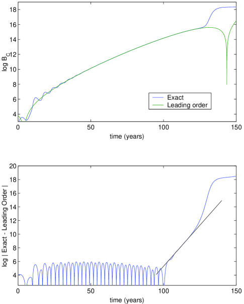
Figure 2: Top panel: comparison of the leading order prediction for $B_{C}$ and the actual computed solution. Bottom panel: the logarithm of the difference of the two curves, showing the onset of instability commencing at about $t=100$

Perhaps the most significant feature to note is the sharp dip of the leading order curve in the top panel at about $t=143$. This reflects the zero crossing of the sine function in (19). There is a second dip at $t=3$ but this is in the interval of initial adjustment as the solution evolves from the given initial conditions onto the “manifold” defined by the exponential solution. Of necessity, a complex exponential solution invalidates itself; even discounting that predicted negative values for the various variables are meaningless, that the terms assumed largest in the equations become arbitrarily small is inconsistent. While we are not yet, based on analysis, able to say what becomes of the solution subsequently, we nonetheless can give a definite estimate for the breakdown time, namely $T=\pi/\Im(\mu_{0})$, here $139.5$ years. It is fundamentally this half-period dictated by the root of the quintic that sets the basic duration of economic growth.

Late in the cycle there is the noted onset of instability, whose growth rate is much faster than $\Re(\mu_{0})$, and this precipitates the ultimate (nonlinear) collapse. As remarked above, that fatal instability cannot occur early in the cycle; the conditions for its growth are unfavorable then. So we may accept $T$ as a leading order approximation of the duration of the economic growth cycle (or equivalently, the time until collapse), with modest correction of that based on a detailed analysis of the transition to collapse, briefly limned in §3.3.

Finally, while (19) does match the computation very well, that comparison rests upon two empirical parameters. A more exacting, parameter-free test is desirable. For this purpose, (12-13) suggest that one compute the ratio of $F_{L}/F_{D}$, as this should approach a constant. That value of that constant is a specific prediction from the solution of the overdetermined linear set noted in the first part of §3. For $s=0.285$, the exact values of the relevant coefficients are found to be

$$F_{L}^{(0)}=15.935787+0.32483068\,i\qquad F_{D}^{(0)}=15.050902+0.23250923\,i\,.$$

Converting these complex results to equivalent real-valued solutions gives the ratio of the moduli of these two complex numbers as the desired constant, $1.058886$. The ratio of $F_{L}/F_{D}$, divided by that prediction, is plotted as the “raw” curve in Figure 3. That result is not seen to approach unity. The reason is that the complex results also determine a phase shift of $F_{L}$ with respect to $F_{D}$, as reflected in the arguments of their respective sine functions following conversion to real form. For the given parameters, deposits at a given time should be compared to loans slightly more than two and a half months earlier; deposits lag loans. That result (“phase adjusted”) conforms to expectation extremely well; the ratio levels off to within a few parts in $10^{4}$ of unity. (The later sharp upsweep of the curve marks the transition to collapse.) The theory is vindicated.

This phase correction points up a needed revision in the proposed estimate of $T$. Really one should solve the augmented $6\times 6$ system, as was done for the entries above, and the phases of the five fields relative to $B_{C}$ determined. The complete results of this exercise for the unstable case here are given in Table 3, expressed in real form. The nearest zero crossing over this full set marks a tighter upper bound on the duration of growth, always less than half a period. Here (and in most cases) that restriction comes from the phase shift for wages, $W$, and the constrained period is $T^{*}=125.74$ years. For smaller values of $T$, this restriction can become a significant relative decrease. Nonetheless, for simplicity, in the remainder of the paper we continue to cite the formula for the elementary estimate, $T$, as an explicit representation for the phase correction is not immediately revealing.

Table 3: Scale amplitudes and phases for the unstable (complex) version of the asymptotic solution in (10 - 17) that matches the model with parameters as given in Table 1 except for $s=0.285$

variable	amplitude	phase (years)
$B_{PL}^{(0)}$	$0.5949050$	$-0.0277274$
$F_{D}^{(0)}$	$15.0526978$	$0.6862392$
$F_{L}^{(0)}$	$15.9390976$	$0.9054319$
$W^{(0)}$	$23.8111979$	$13.7830358$
$P_{C}^{(0)}$	$31.8161573$	$12.8275901$

To reiterate an earlier observation, we might have launched this model economy with a million dollars in firm loans outstanding and one dollar in the firm’s deposit account. Or the reverse. And yet after a modest interval, that ratio of firm loans to firm deposits (suitably lagged) approaches parity ($1.0588..$), and without regard to any other initial variable, such as the interest rate, or worker salary, or the employment rate! The more general import of this is the suggestion that the most useful economic indices will generally be ratios of time-lagged aggregate quantities. Which ratios are of most diagnostic value will depend on the quality and frequency of available datasets. Optimal lags must be discovered empirically.

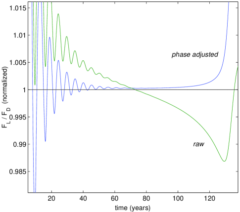
Figure 3: A second test of the asymptotic theory: the ratio should approach unity.

3.2 Stable solution

Turning to $s>s_{crit}$, we take $s=0.3$ and find the largest root is $\mu_{0}=0.13171713$. We can here anticipate a correction to the leading order form

$$B_{C}\sim B_{C}^{(0)}\,\exp(\mu_{0}\,t)+B_{C}^{(1)}\,\exp(\nu_{1}\,t)\,.$$ (20)

For Figure 4 the coefficients $B_{C}^{(0,1)}$ are determined by a least squares fit. Note the oscillatory residual, once these two are removed, which is also exponentially growing, but is subdominant to the other two. Empirically this solution is stable; growth persists indefinitely. To prove its linear stability would be a tedious exercise but also a weaker result than desired. Linear stability shows only that the solution is stable to infinitesimal disturbances where this solution has in fact finite amplitude stability; it recovers from observable disruptions. A yet stronger result would be a demonstration of “global stability”, meaning that this solution is the universal long term outcome for all possible initial economic states. But that is easily shown to be false by counterexample as indicated in Figure 5, where we introduce a bifurcation induced now by $v$, the capital-output ratio, rather than $s$ as above, and track the behavior of $F_{D}$.

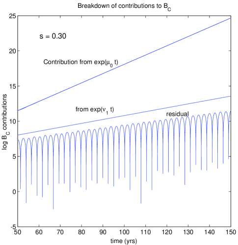
Figure 4: Dissection of the exact solution in terms of (20).

The initial computation uses $v=2.9$, which is still in the unstable complex exponential regime. The computation is then halted at $t_{1}=94.16736$ and again at $t_{2}=94.16748$. Each of these two interrupted computations is then continued but with $v=2.7263$, for which $\mu_{0}$ is real and hence a stable growing solution exists as that above.

But note that while the first computation carrying on from $t_{1}$ (upper curve) does eventually approach the stable growing solution with predicted growth rate $\mu_{0}=0.1167$, the second one commencing from $t_{2}$ (lower curve) ultimately ends in collapse. We can infer that there is a particular value $t^{*}$ in the open interval $(t_{1},t_{2})$ that does neither, but rather continues along the indicated dashed line with slope $\mu_{1}=0.05428$. This is the second positive root of the quintic; it is an unstable solution. The set of all possible initial conditions that yield this second solution constitutes a border in the eight-dimensional space of initial conditions; dividing solutions that grow indefinitely at rate $\mu_{0}$ from those that collapse. As the present computation hints, conditions that yield the latter are uncommon. In effect, only when the initial state is such that things are already headed towards collapse is that scenario likely to continue.

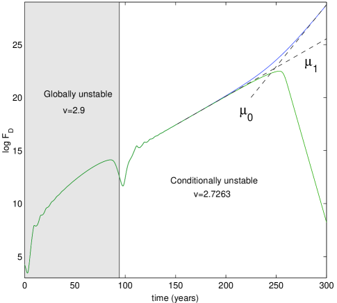
Figure 5: A slight perturbation of initial conditions to show that either immediate collapse or stable long term growth is possible.

3.3 Collapse and predictability

The late stage evolution of the solution heading for a collapse is as follows. First note that $\pi_{r}$ diverges as a negative definite exponentially growing function and hence the functions $Inv$, $\tau_{RL}$ and $\tau_{LC}$ quickly saturate at $0$, $3$, and $\infty$ respectively. Also $\lambda$ is a positive definite exponentially decaying function and so quickly $Ph$ saturates at $-4/100$. We have then in addition that $g=-\delta$. (These simplifications are easily justified as self-consistent after the fact.)

It follows that

$$B_{C} \sim bc_{0}+bc_{1}\,\exp(-t/\tau_{RL})$$ (21)

$$F_{L} \sim fl_{1}\,\exp(-t/\tau_{RL})$$ (22)

$$Kr \sim kr_{1}\,\exp(-\delta\,t)$$ (23)

$$\lambda \sim \lambda_{1}\,\exp(-(\alpha+\beta+\delta)\,t)$$ (24)

Next one solves for the pair $P_{C}$ and $W$. This pair is exactly soluble on the substitutions noted above and yields

$$P_{C} \sim \exp((\exp(-(\alpha-Ph+\mu)\,t)\,c_{1}-c_{2})/(\alpha-Ph+\mu)+(1-t)/\tau_{Pc})$$ (25)

$$W \sim c_{1}(s-1)\,a_{0}\,\tau_{Pc}\,\exp((Ph-\mu)\,t)\,P_{C}(t)$$ (26)

where $\mu=\omega\,(\alpha+\beta+\delta)$. Notice the exponential within the exponential in the form for $P_{C}$. These two results are easily confirmed by using simulation results to plot $P_{C}/W\,\exp((Ph-\mu)\,t)$, which quickly saturates to a constant (and allows immediate determination of $c_{1}$).

This leaves one to solve for $F_{D}$ and $B_{PL}$. There are several exponentials contributing to the solution for each but, for the parameters as given in the standard model, all of these except the leading contribution can be safely neglected leaving

$$F_{D}\sim fd_{0}+fd_{1}\,\exp(-t/\tau_{RL})\qquad B_{PL}\sim bp_{0}+bp_{1}\,\exp(-t/\tau_{RL})\,.$$ (27)

It is an involved exercise to work out the relations among the various coefficients in these asymptotic forms but it is anyway instructive to note that $bp_{0}=cst/99$, where $cst$, recall, is the conserved quantity $F_{L}(t)-F_{D}(t)-B_{PL}(t)-W_{D}(t)$.

From these functional forms, one can derive the previously asserted exponential divergence of $\pi_{r}$ and so the set constitutes a valid asymptotic solution for the set of eight differential equations. Unlike the previous solution however, this solution does not lead to any characteristic polynomial whose coefficients depend on the parameters in the problem and so it does not have an associated regime diagram like that in later Figure 9. Rather, this solution exists for all parameter settings.

In Figure 6 the prediction from (26) (right hand dashed curve) is compared to the exact solution for the same unstable case as in §3.1, where $s=0.285$. (As before, the needed parameters are obtained from a numerical fit. These are $c_{1}=-1654.10346$ and $c_{2}=-8.74399851$.) In addition the predicted exponential growth from (14) is plotted. It is seen that the two results cover nearly the entire span of time. The narrow time interval of about $[110,125]$ is the transition from one asymptotic form to the other.

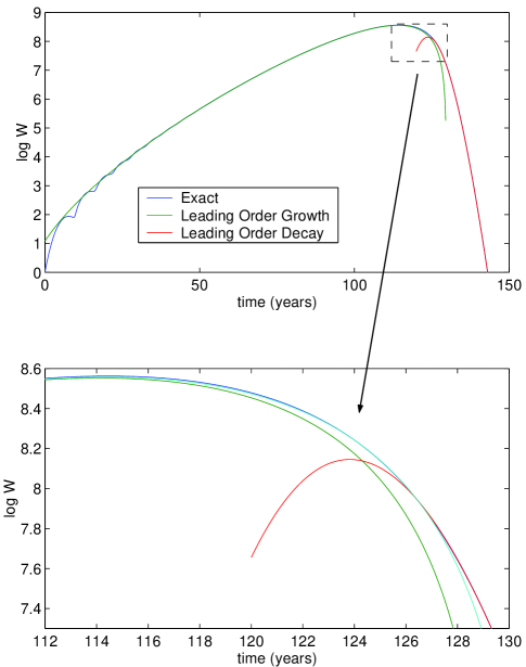
Figure 6: Prediction for $W$ in the terminal collapse.

This bridge is effected by the same instability denoted by the straight line segment in Figure 2. In first approximation, the slope of that line emerges as the eigenvalue of a particular matrix. As an expedient substitute for that calculation, the slope was determined ex post facto to be about $0.24$. The sum of this growing transient $c_{3}\,\exp(0.24t)$, added to the complex exponential solution, is plotted as a dash-dot line in the lower panel (but not the upper) of Figure 6. One observes that the sum intersects the second dashed curve (the decay solution) tangentially. This is a simple graphical construction of what would emerge from the method of matched asymptotic expansions. By means of that formalism the amplitudes and phase, all here determined empirically, are instead found deductively from the requirement that successive parts of the solution be smoothly joined.

This view of the solution raises the issue of sensitivity to initial conditions. Over most of the cycle, evolution of the two exponential solutions, growing and decaying, is perfectly stable. Any variability in time scale for collapse must therefore arise from either: (1) the initial transient adjustment as the solution tries to lock on to the growing solution, or (2) the timing of the trigger for the second transient parasitic solution that acts as the bridge from one to the other exponential.

Figure 7 is instructive in this regard. Here one hundred simulations are plotted with the eight initial conditions in Table 2 for each run perturbed by a fractional change of $\delta_{k}$ for $k=1\ldots 8$, where $\delta_{k}$ is a normal random variable of zero mean and standard deviation $\sigma=0.01$. The results are plotted each with an individually adjusted time shift $\Delta t=c_{2}/\Im(\mu_{0})$ where $c_{2}$ is the phase in (19), computed by a log least squares fit on the range $t=[60,90]$. This amounts to synchronizing the time in each realization by using for a reference the asymptotic exponential solution to define the origin, $t=0$. With this timing shift, the average of all simulations is equivalent to starting at $t=-3.98$ years and with a standard deviation of $\sigma=1.12$ years. It takes, in other words, on average about four years to get locked into a long period cycle of growth for initial conditions in this neighborhood.

For clarity, each realization of $B_{C}$ is also scaled by the amplitude of the associated asymptotic solution (19) at $t=70$ in the shifted frame, that is, $|B_{C}^{(0)}|\,\exp(\Re(\mu_{0})\,(70-\Delta t))$. That scaling is significant because the ensemble of computed values of $B_{C}$ spans two orders of magnitude by $t=120$, a huge sensitivity to initial conditions indeed! But now the asymptotic rescaling and shift make it abundantly clear that the onset of collapse is rigidly locked in time on adopting (19) to define the time origin of the growth cycle. The latter synchronization is a manifestation of nonlinearity and can be seen as a consequence of the associated matched asymptotic expansion; the collapse cannot be adjoined to the growth phase at an arbitrary point in the cycle. Rather, the required smoothness of connections simultaneously in not just $B_{C}$, but all eight variables, singles out a unique point, late in the cycle, where the match must be made. The piece that connects the two exponential solutions contains a subdominant contribution that reflects the influence of particular initial conditions. The conclusion is that the leading order sensitivity of the solution timing to initial conditions is solely the varying interval it takes for locking onto the growth cycle. Once this is achieved, the timing of the collapse is preordained.

On this view one should describe collapse as taking one of two asymptotic mathematical forms; the immediate collapse and the deferred collapse. The first is the solution given in (21-27). The second is a more involved structure, a so-called “uniform asymptotic expansion,” consisting of the solution stated in (10-17) from §3.1, using canonical initial conditions at $t=0$ (scale amplitudes and phases for the particular parameters, as in Table 3, with free parameters of $[B_{C}^{(0)},\Delta t_{B_{C}},K_{r}^{(0)}]$ determined by the eight initial conditions), and switching at late time to (21-27) by means of a correction term that effects the match to leading order. It is then only a question of which of these two solutions is the “nearer” for a given set of initial conditions in the eight-dimensional space of Table 2.

With regard to duration of the economic cycle as a function of variation in the initial conditions, this is a “regular” perturbation; the value of $\sigma=1.12$ is about a one percent change in the realized value of $T$, of the same order as the scale of the perturbation of initial conditions. Of course the definition of $T$ is somewhat ambiguous depending what characteristic feature of the solution at late time is chosen but an average value of $130$ years is plausible and this differs modestly from the leading order estimate of $\pi/\Im(\mu_{0})$.

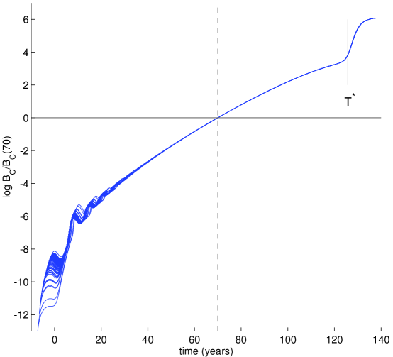
Figure 7: Sensitivity of the solution to perturbation of the initial conditions.

Note from the plot that the phase-adjusted refinement of this, $T^{*}$, is an excellent predictor for the transition to collapse. This accuracy holds up for shorter cycles as well, as shown in Figure 8, with parameters varied from Table 1 in a Monte Carlo run. This parameter set results in 60 years of growth before collapse, similar in duration to the postwar private sector debt run-up from 1945 through 2008. The plot is similar to Figure 3, with another time-lagged ratio, $B_{P}/B_{C}$, normalized so that the predicted asymptotic limit for the growth phase is again unity.

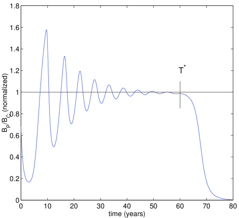
Figure 8: A shorter period of growth, with collapse still accurately indicated by $T^{*}$.

3.4 Regime diagrams

Returning once more to the focus on the single bifurcation parameter $s$, we can by aid of (18) quickly sketch out a regime diagram, shown in Figure 9. To the right, the dominant root of $\mu$ is real and the solution of §3.2 is the outcome for most initial conditions. In the middle (light gray), the leading root is a complex pair and the usual outcome is the “deferred collapse”, with a period of growth (§3.1) followed by a quick collapse (§3.3). To the left (dark gray), all roots of $\mu$ lie in the left half plane so no exponential growth is possible and all initial conditions lead to collapse. (Note that the apparent bifurcation for small $s$ is nugatory. The two leading roots are real however the largest of these is still less than zero, violating the assumption that the exponential terms dominate, e.g. the constant sum of $F_{L}-F_{D}-B_{PL}-W_{D}$.)

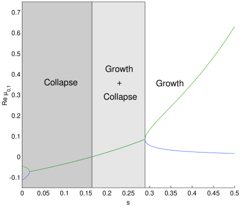
Figure 9: Bifurcation from stability to instability induced by the return to capital, $s$.

One would like to understand the general sensitivity of this system to bifurcations such as this one in $s$ (or $v$). The order of the characteristic polynomial for $\mu$, quintic, is a function of the form of the differential equations; modifying parameters cannot change that. But as with $s$, so too variations of other parameters may induce bifurcations. There are a large number here and in the remainder we briefly examine the influence of ten: $[\tau_{B},\tau_{W},r_{L},\tau_{PC},r_{D},s,v,\alpha,\delta,\beta]$. (It would be possibly instructive — and feasible — to enrich this space with sixteen more; the parameters in the four generalized exponential functions for $\tau_{RL}$, $\tau_{LC}$, $\mbox{Inv}(\pi_{r})$, and $\mbox{Ph}(\lambda)$.)

This is rather too much freedom to exploit and it is useful first to undertake a more limited exploration; to vary each of the ten parameters singly and compare results. A natural way to make this comparison is to replace a candidate variable $x$ whose value in the standard model is $x_{0}$ with $\nu\,x_{0}$, and allow $\nu$ to vary from $1/4$ to $4$ in equal logarithmic steps. For a number of these, a factor of four either way lies well outside the range of real world plausibility but the exploration is for the moment a purely formal one.

The results in Figure 10 show that the parameters $\tau_{B}$ and $\tau_{W}$ for example have negligible influence on the roots. The three that are most sensitive are the return to capital $s$, with a bifurcation to stability for increasing $s$ at $0.289$, for a decreasing capital-output ratio $v$ at $2.797$, and a decreasing interest rate on loans $r_{L}$ at $0.038$. (Each of these values is readily verified with short time stepping runs a bit beyond the point of bifurcation, confirming that the ten parameter coding of the characteristic polynomial is correct.) Other parameters, such as $\tau_{PC}$ do induce a bifurcation, but only for a relatively large change in value (about a factor of two).

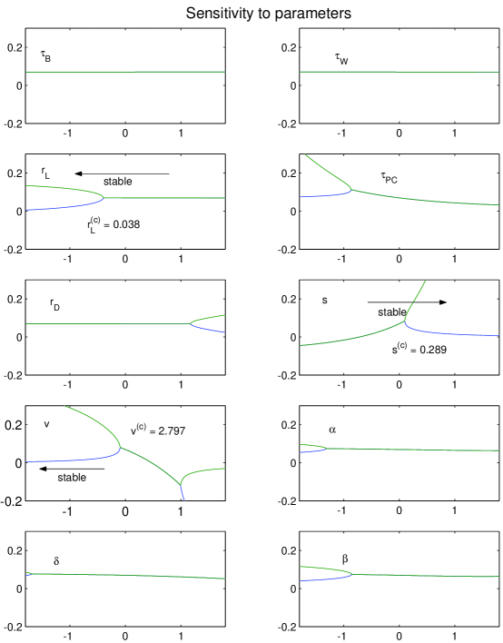
Figure 10: Sensitivity of bifurcations to the ten model parameters individually

While $r_{L}$ is a relevant factor, for both simplicity and graphical reasons we confine attention to a two-dimensional subspace, that of $[s,v]$. Figure 11 illustrates the border of stability in this plane, with axes as those in Figure 10. The vertical line corresponds to the slice shown in panel six of Figure 10, the horizontal line to panel seven. Their intersection is the standard model. The log of the leading order estimate of $T=\pi/\Im(\mu_{0})$ is contoured in color. Note that the odd behavior in the upper right hand corner, where the period becomes extremely short, reflects the return to capital $s$ approaching unity.

The border separating stable from unstable growth makes intuitive sense. Its positive slope shows that, as the economy becomes more capital intensive (increasing $v$), the minimal return to capital, $s_{crit}$, that ensures stability is monotone increasing. Near the center of the plot, that relation is approximately $s_{crit}=1.12\,s_{0}\,(v/v_{0})^{1.07}$. Moreover, there is a critical value of $v$ above which the economy must always collapse directly.

Setting aside phase lags in the complex case, when $\Re(\mu)=\beta+\alpha$, from (15) prices are asymptotically constant. This is shown by the dashed line. To the left the economy is inflationary, prices of goods rise; to the right deflationary. So in this model, and quite likely much more generally for debt-based economies, inflation is stabilizing. Furthermore workers here enjoy a rising standard of living (until a collapse), with wages in constant dollars growing in lockstep with productivity gains, as in the US from 1947 to 1973. This holds even in a deflationary regime and with falling wages (to the right of the dash-dotted line), albeit the period of growth then becomes very short.

Also note in this figure the red dashed line that demarcates a critical state where $F_{D}=0$, the firm has no assets at all (but the bank continues to advance it loans on the Micawberish promise of future earnings). This is an intrinsic model limit; values of $(s,v)$ above the red line lead to negative asymptotic values for $F_{D}$. As remarked earlier, realizable models in general are those for which the entire set $[B_{PL}^{(0)},F_{L}^{(0)},F_{D}^{(0)},W^{(0)},P_{C}^{(0)}]$ yields non-negative results. In the particular slice shown here it simply happens to be $F_{D}^{(0)}$ that defines the border of allowed parameter space.

Below this line in the allowed region, firm assets ($F_{D}$) are always less than firm liabilities ($F_{L}$) — the firm perpetually runs in the red. This is not unexpected in the (complex) regime of mixed growth and collapse where, as in Figure 3, the appropriate phase lag is used, but it remains true even in the pure growth regime, where there is no phase lag. But recall that at leading order the linear coefficients satisfy $W_{D}^{(0)}+F_{D}^{(0)}=F_{L}^{(0)}-B_{PL}^{(0)}$ and since all terms are constrained to be positive definite for a consistent model, then necessarily $F_{D}^{(0)}\leq F_{L}^{(0)}$. If worker loans were introduced to the model we would have only the weaker aggregate inequality that $W_{D}^{(0)}+F_{D}^{(0)}\leq F_{L}^{(0)}+W_{L}^{(0)}$ and one or the other could have assets greater than liabilities, but not both.

Reincorporating $r_{L}$, the wedge-shaped region typified by deferred collapse becomes a volume whose varying extent in that third dimension could next be explored. With the addition of further parameters, a complicated hypervolume results but, again, the main operative constraints on stability as suggested by Figure 10 remain the subspace spanned by $[s,v,r_{L}]$.

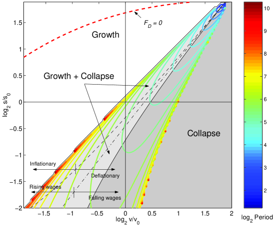
Figure 11: Bifurcation in the two-dimensional subspace of $[s,v]$, with shading as in Figure 9. Contours indicate the approximate period, $T$, of economic growth but these apply only in the light gray region.

For completeness sake it should be noted that the border separating light from dark gray, $\Re(\mu_{0})=0$, constitutes another class of solutions, these exhibiting algebraic, rather than exponential, behavior. Also in this spirit are solutions that lie at borders in the space of initial conditions as noted in §3.2, rather than in parameter space. But border solutions of either kind are of limited relevance as they are unstable to an infinitesimal perturbation.

3.5 Model Robustness

Another aspect of the model bears comment. One would like to be sure that the identification of stable and unstable regimes is a robust one. Here we can look to the forms chosen for $a(t)$ and $N(t)$ from concern that the arguments given earlier, which trade heavily on the properties of exponential functions, point to an implausible sensitivity on having exactly an exponential form for the underlying variables $a$ and $N$. While one can argue that an exponential growth model is justified for population (excepting inconveniences such as wars and plagues), there is not really much to be said in its defense for $a(t)$ except that historical data show a concave upward trend.

So one might instead try a replacement for both of these in the form of algebraic growth:

$$a=a_{0}\,(t_{0}+\alpha\,t)^{\nu}\qquad N=N_{0}\,(t_{0}+\beta\,t)^{\nu}\,.$$

By suitable adjustment of the exponent and constants, each of these can be made to give curves similar enough to data over a time span of say, $50$ years, that a model based on these latter forms had better give qualitatively similar results. (The choice of $\nu=5/2$ is reasonable for matching the standard case.)

Briefly, this form does largely recapitulate the results above (and with surprisingly little change in e.g., $s_{crit}$). One can conjecture that the weak requirement of merely a concave upward form for $a$ and $N$ suffices. One could strengthen this argument for robustness further by looking to equivalent conclusions for variation in the functional form of $G$, the all purpose exponential here for $\tau_{RL}$ and allied functions, but there are not likely to be any surprises in that direction either.

4 Conclusions

At times mathematical manipulations can obscure, not reveal, the meaning of a model. So it bears emphasizing that the central points here are simply expressed. Any economy has a finite capacity for carrying aggregate debt. How much debt depends upon various factors, notably among them the three earlier cited: interest rate, return to capital, and the capital to output ratio. In a stable Schumpeter economy all the relevant economic indicators march together in synchrony. When the debt burden exceeds the carrying capacity of the economy, the hallmark is the necessary lag of key variables. We have seen this in Figure 3. Recall that deposits lag loans and only by reason of that delay is it possible to sustain speculative investment in that model economy.

It is evident this relation must be unidirectional in time; it would be nonsensical were the time ordering reversed. So much is clear with no need of mathematical argument. Indeed, judging from the byzantine result of Appendix A for the phase of wages, $W$, it is likely not even possible to prove such a phase relation between $F_{L}$ and $F_{D}$. And for the model here it may not even be true for all possible parameter values. But, were loans to lag deposits, we should simply conclude the model was in that parameter range irrelevant to the real world.

So Schumpeter’s “creative destruction” is a healthy aspect of capitalism only when the economy in which it operates has adequate capacity to sustain the associated debt and that does not automatically come about from the invisible hand of Adam Smith. It requires no great leap of faith to conclude that Ponzi finance must inevitably overwhelm the carrying capacity of any economy.

To be sure, the model here is at best a “lumped parameter” description of a complicated nonlinear system. One is mindful from the Sonnenschein Mantel Debreu theorem that macroeconomic modeling has in key respects only a tenuous relation to microeconomic models and so it is fair to question how robust are the conclusions drawn here; whether the equations that compose this model are even an appropriate representation of aggregate behavior. The best line of argument in defense is probably to be had from appeal to empirical time series.

Michael Hudson has written often of the central role of debt in economies since antiquity, particularly underscoring Marx’s incisive critique of debt in capitalism, emphasizing its exponential growth Hudson (2010) as well as its ratcheting quality: “… every U.S. business recovery since WW II has taken off with a higher level of debt. That means debt service — the monthly ‘nut’ you have to cover — has become much higher with each recovery.” Hudson (2009) The ultimately catalytic role of mounting debt in precipitating collapse is pungently expressed by Hudson in his epigram “debts that can’t be paid won’t be.”Hudson (2012)

Keen has expressed this dynamic through the time rate of change of debt contributing to the aggregate demand. And what emerges then in the system here defined by (1 – 8) is rapid evolution onto a manifold, to use the nomenclature of nonlinear dynamical systems.

The typical occurrence of “slow” manifolds as illustrated in textbook problems for a system of two or three first-order nonlinear differential equations has one identify variables as either “fast” or “slow”. The former are said to be “slaved” to the slow variables, and this signifies that equations for the fast variables have the time derivative eliminated, leaving an algebraic relation that defines fast in terms of slow. This relation fixes in turn the structure of the slow manifold, normally by an iterative process that may or may not give a convergent global representation. Commonly the fast variables evolve exponentially in time while evolution on the manifold is algebraic, so the disparity in time scales is great.

Here the fast evolution is exponential in time, but so is the slow evolution; there is only a difference in rates and hence the decaying epicycles as in Figure 8 remain apparent. The approach here aims also at a exposing a manifold, but the resulting uniform asymptotic expansion of §3.3 is more correctly thought of as a closely related “inertial” manifold.

That aim has largely been achieved. The one technical omission, of a detailed match of two exponential solutions, is not likely to be very revealing. It would give a more refined value for $T^{*}$, but one hardly differing from the conceptually much simpler, and substantially accurate, phase-corrected value already defined.

What emerges in a broader sense is an understanding that the manifold reflects the centrality of debt in economic systems. The economy is indeed “slaved” to debt, not merely in the narrow technical sense of dynamical systems, but in human terms as well. Atop this structure lie the epicycles that offer the great economic sport of daily life, the engaged players blithely unaware of a slower clock, ticking away inexorably on a multi-decadal time scale, the hidden alarm long ago set.

Appendix A Correction for $T^{*}$

Typically the largest phase shift, which dictates the corrected period $T^{*}$, is that for $W$. In terms of the complex root $\mu_{0}$, that phase shift can be computed exactly according to:

$$W^{(0)}=\frac{\mu_{0}\,(s-1)}{\alpha+\beta+\delta}\,\left(1+\tau_{P_{C}}\,\left(\mu_{0}-\alpha-\beta\right)\right)\,\frac{N(\mu_{0},\gamma)}{D(\gamma)}$$

where

$$N(\mu_{0},\gamma) = 6125\,(5\,{\rm e}^{2})^{1/7}\,(\mu_{0}+2)\,\gamma^{26}+175\,(5^{4}\,{\rm e})^{1/7}\,(6\,\mu_{0}+13)\,\gamma^{20}+75\,(3\,\mu_{0}+7)\,\gamma^{14}$$

$$+735\,\mu_{0}\,(5^{17}/{\rm e})^{1/21}\,\gamma^{12}+105\,(5^{5}/{\rm e}^{4})^{1/21}\,(6\,\mu_{0}+1)\,\gamma^{6}+9\,(5^{2}/{\rm e})^{1/3}\,(3\,\mu_{0}+1)\,,$$

$$D(\gamma) = (7\,(5^{4}\,{\rm e})^{1/7}\,\gamma^{6}+3)\,(25\,\gamma^{14}+3\,(5^{2}/{\rm e})^{1/3})\,,$$

$$\gamma = \left(v\,\left(\alpha+\beta+\delta\right)\right)^{1/21}\,.$$

The phase shift is then $\tan^{-1}(\Im(W^{(0)})/\Re(W^{(0)}))$ and the scale amplitude is $|W^{(0)}|$.

Appendix B Full asymptotic expansion; Origin of the Great Moderation

A more complete version of (10 - 17) assumes the form:

$$\tilde{B}_{C} \equiv B_{C}-\frac{\tau_{LC}^{(0)}}{\tau_{RL}^{(0)}}\,\frac{r_{D}\,cst}{r_{D}-r_{L}}\sim B_{C}^{(0)}\,\left(\exp(\mu_{0}\,t)+B_{C}^{(1)}\,\exp(\nu_{1}\,t)+B_{C}^{(2)}\,\exp(\nu_{2}\,t)\right.$$ (28)

$$\quad\quad\left.+B_{C}^{(3)}\,\exp((2\nu_{1}-\mu_{0})\,t)+B_{C}^{(4)}\,\exp((\nu_{1}+\nu_{2}-\mu_{0})\,t)+\ldots\right)$$

$$B_{PL} = B_{C}^{(0)}\,\left(B_{PL}^{(0)}\,\exp(\mu_{0}\,t)+B_{PL}^{(1)}\,\exp(\nu_{1}\,t)+B_{PL}^{(2)}\,\exp(\nu_{2}\,t)\right.$$ (29)

$$\quad\quad\left.+B_{PL}^{(3)}\,\exp((2\nu_{1}-\mu_{0})\,t)+B_{PL}^{(4)}\,\exp((\nu_{1}+\nu_{2}-\mu_{0})\,t)+\ldots\right)$$

$$\tilde{F}_{L} \equiv F_{L}-\frac{r_{D}\,cst}{r_{D}-r_{L}}\sim B_{C}^{(0)}\,\left(F_{L}^{(0)}\,\exp(\mu_{0}\,t)+F_{L}^{(1)}\,\exp(\nu_{1}\,t)+F_{L}^{(2)}\,\exp(\nu_{2}\,t)\right.$$ (30)

$$\quad\quad\left.+F_{L}^{(3)}\,\exp((2\nu_{1}-\mu_{0})\,t)+F_{L}^{(4)}\,\exp((\nu_{1}+\nu_{2}-\mu_{0})\,t)+\ldots\right)$$

$$\tilde{F}_{D} \equiv F_{D}-\frac{r_{L}\,cst}{r_{D}-r_{L}}\sim B_{C}^{(0)}\,\left(F_{D}^{(0)}\,\exp(\mu_{0}\,t)+F_{D}^{(1)}\,\exp(\nu_{1}\,t)+F_{D}^{(2)}\,\exp(\nu_{2}\,t)\right.$$ (31)

$$\quad\quad\left.+F_{D}^{(3)}\,\exp((2\nu_{1}-\mu_{0})\,t)+F_{D}^{(4)}\,\exp((\nu_{1}+\nu_{2}-\mu_{0})\,t)+\ldots\right)$$

$$W = B_{C}^{(0)}/K_{r}^{(0)}\,\left(W^{(0)}\,\exp((\mu_{0}-\beta)\,t)+W^{(1)}\,\exp((\nu_{1}-\beta)\,t)+W^{(2)}\,\exp((\nu_{2}-\beta)\,t)\right.$$ (32)

$$\qquad\qquad\left.+W^{(3)}\,\exp((2\nu_{1}-\mu_{0}-\beta)\,t)+W^{(4)}\,\exp((\nu_{1}+\nu_{2}-\mu_{0}-\beta)\,t)+\ldots\right)$$

$$P_{C} = B_{C}^{(0)}/K_{r}^{(0)}\,\left(P_{C}^{(0)}\,\exp((\mu_{0}-\beta-\alpha)\,t)+P_{C}^{(1)}\,\exp((\nu_{1}-\beta-\alpha)\,t)+P_{C}^{(2)}\,\exp((\nu_{2}-\beta-\alpha)\,t)\right.$$ (33)

$$\left.+P_{C}^{(3)}\,\exp((2\nu_{1}-\mu_{0}-\beta-\alpha)\,t)+P_{C}^{(4)}\,\exp((\nu_{1}+\nu_{2}-\mu_{0}-\beta-\alpha)\,t)+\ldots\right)$$

$$K_{r} = K_{r}^{(0)}\,\exp((\alpha+\beta)\,t)\,\Bigl{(}1+\frac{9\,\pi_{r}^{(1)}}{4\,(\nu_{1}-\mu_{0})}\,\exp((\nu_{1}-\mu_{0})\,t)+\frac{9\,\pi_{r}^{(2)}}{4\,(\nu_{2}-\mu_{0})}\,\exp((\nu_{2}-\mu_{0})\,t)$$ (34)

$$+\frac{9\,\pi_{r}^{(3)}}{4\,(2\nu_{1}-\mu_{0})}\,\exp((2\nu_{1}-\mu_{0})\,t)+\frac{9\,\pi_{r}^{(4)}}{4\,(\nu_{1}+\nu_{2}-\mu_{0})}\,\exp((\nu_{1}+\nu_{2}-\mu_{0})\,t)+\ldots\Bigr{)}$$

$$\lambda = \lambda^{(0)}\,\Bigl{(}1+\frac{9\,\pi_{r}^{(1)}}{4\,(\nu_{1}-\mu_{0})}\,\exp((\nu_{1}-\mu_{0})\,t)+\frac{9\,\pi_{r}^{(2)}}{4\,(\nu_{2}-\mu_{0})}\,\exp((\nu_{2}-\mu_{0})\,t)$$ (35)

$$+\frac{9\,\pi_{r}^{(3)}}{4\,(2\nu_{1}-\mu_{0})}\,\exp((2\nu_{1}-\mu_{0})\,t)+\frac{9\,\pi_{r}^{(4)}}{4\,(\nu_{1}+\nu_{2}-\mu_{0})}\,\exp((\nu_{1}+\nu_{2}-\mu_{0})\,t)+\ldots\Bigr{)}\,.$$

The significant generalization here is that quantities previously assumed constant now incorporate the transient corrections as well, as seen in the last expression above for $\lambda(t)$. The defining transient is taken to be in the variable $\pi_{r}$, now written in the form

$$\pi_{r}=\pi_{r}^{(0)}+\pi_{r}^{(1)}\,\exp((\nu_{1}-\mu_{0})\,t)+\pi_{r}^{(2)}\,\exp((\nu_{2}-\mu_{0})\,t)+\pi_{r}^{(3)}\,\exp((2\nu_{1}-\mu_{0})\,t)+\pi_{r}^{(4)}\,\exp((\nu_{1}+\nu_{2}-\mu_{0})\,t)+\ldots\,.$$ (36)

From this latter, the corresponding transient amplitudes in both $\lambda$ and $K_{r}$ above are immediately expressed in terms of $\pi_{r}^{(k)}$ as indicated. Similar transient forms are easily deduced for the auxiliary quantities $[g,\tau_{RL},\tau_{LC},Inv,Ph]$. Though the variables $\pi_{r}^{(k)}$ are ultimately eliminated in favor of $B_{C}^{(k)}$ by use of (9), which defines $\pi_{r}$, they are extremely useful as an intermediate placeholder for a tractable formulation of the problem.

Here for simplicity we restrict attention to the case of real $\mu_{0}$. (The analysis is similar for the complex case.) Each of (28-35) is a formal asymptotic infinite series about $t\to\infty$. While the radius of convergence of an asymptotic series is zero, such series are nonetheless extremely useful, just not all the way to the origin $t=0$ in the present case.

The earlier noted degeneracy of equations for $dW/dt$ and $dP_{C}/dt$ is true only in leading order. At next order each must separately be enforced. The requirement that the series above hence satisfy (1 – 8) and (9) at second order yields an eleventh degree polynomial in $\nu$ whose coefficients depend, not only on the explicit parameters in Table 1, but on the value of $\mu_{0}$ as well. Four of the roots of this polynomial are always $\mu_{0}$ but these are discarded, so the reduced polynomial is seventh degree.

This polynomial is too complicated to carry along the general ten parameter dependence of the coefficients, even with the aid of symbolic manipulation, hence we turn now to the particular case of $s=0.3$ considered in §3.2 for which the leading roots are found to be

$$\nu_{1}=0.05496705\qquad\nu_{2}=0.04054906+1.22315328\,i\,.$$

Of the seven roots of $\nu$, four are simply slight perturbations of the quintic roots noted in the main body of the paper. Here for comparison e.g., $\mu_{1}=0.05540080$. But $\nu_{2}$ and its conjugate companion have no match from leading order; these are new spontaneous solutions of the system. The next two roots are $\nu_{4}=-0.99$ (exactly) and $\nu_{5}=-0.99082495$. The first of this pair can be matched with $\mu_{3}$. The second lacks a match however one observes that perturbing a constant solution and allowing for a single common exponent correction for all variables yields a double root of $-1$, that is, solutions of $\exp(-t)$ and $t\,\exp(-t)$, so the pair $\nu_{4,5}$ would seem to be a splitting of this repeated root. Finally $\nu_{6,7}$ match with $\mu_{4,5}$.

Where the leading order asymptotic expansion in §3 had only two free real parameters, $[B_{C}^{(0)},K_{r}^{(0)}]$, the form above has the added $B_{C}^{(k)}$ that accompany the single exponent form $\exp(\nu\,t)$ (note that $B_{C}^{(2)}$, is complex, hence equivalent to two real parameters; amplitude and phase). This development of the polynomial in $\nu$ seems to result in one too many free parameters; seven from the new roots and the two scale parameters introduced in §3. The resolution is that dynamics of the equation for $W_{D}$ have been implicitly incorporated through the accounting identity noted at the beginning of the paper and so nine free parameters are required for a general solution. The expansion above has been truncated at $\nu_{2}$ both for relative compactness of the formulae and because the remaining terms in $\nu_{k}$ are negligible but formally they must be included to constitute a general solution that is an asymptotic expansion of an exact solution of (1 – 8). This exponent partition reflects that the effective dimension of the system is not nine, but five. For the truncated form above, coefficients of remaining terms with superscripts $(1,2)$ and of all terms with superscripts $(3,4)$ can be found in terms of the five parameters $[B_{C}^{(0,1,2)},K_{r}^{(0)}]$.

Note that (28), (30), and (31) address the initial assumption of homogeneity, which led to the identification of the scale parameters $[B_{C}^{(0)},K_{r}^{(0)}]$. Properly incorporated, the conserved quantity redefines the relevant variables for asymptotic expansion, i.e., the equations have to be recast in terms of $[\tilde{B}_{C},\tilde{F}_{L},\tilde{F}_{D}]$.

There is a final subtlety to be noted about the expansion. If one takes the explicit ninth order system defined by (1 - 8) plus the equation for $dW_{D}/dt$ and follows the same analysis, a different polynomial emerges. Terming those roots $\rho_{k}$, then $\rho_{1,2,3}=\nu_{1,2,3}$ but there is an added root $\rho_{4}=0$, which reflects that there is a conserved quantity for the equations, here absorbed in the redefined tilde variables. In addition $\rho_{7,8}=\nu_{5,6}$ but remaining roots $\rho_{5,6}$ (a repeated real root) and $\nu_{4,7}$ differ. Both pairs are at the level of rapidly decaying transients, not in the effective five-dimensional subspace. The discrepancy is resolved by additional terms stemming from recasting the equations in terms of $[\tilde{B}_{C},\tilde{F}_{L},\tilde{F}_{D}]$ to reflect the conservation law, leading to a modification of $\nu_{4,7}$.

Because the general asymptotic solution cannot be carried back to the origin, one could not directly relate a given set of nine initial conditions to an equivalent set of values for the free parameters. This is a minor cavil. One could always evolve the solution from $t=0$ to some moderate value $t_{0}$, where the truncated asymptotic series were judged sufficiently accurate and make the connection there. More to the point is that the mapping from the values of the variables onto the (now) nine free parameters, whether at $t_{0}$ or at the origin, is a nonlinear one and, as already signaled by Figure 5, there is no such real-valued mapping for a certain continuous region in the space of nine variable values. That region constitutes the space of initial conditions that map instead to the collapse solution.

To most easily see the first few correction terms emerge it is convenient to test (35). As usual, this requires an empirical determination of constants, here $\pi_{r}^{(1,2)}$ (with $\pi_{r}^{(3,4)}$ found by a recurrence relation). The first two assume the values

$$\pi_{r}^{(1)}=4.0481601\times 10^{-5},\quad|\pi_{r}^{(2)}|=6.7677858\times 10^{-3},\quad\phi=2.0915926\,$$

where $\phi$ is the phase shift, as in previous instances of the complex exponential. The accuracy of (35) is evident in Figure 12. From the top panel one would say that the solution has locked onto the asymptotic solution at this level by fifteen years. Comparison of two- and four-term expansions suggests that, if a few more terms are kept, reasonable agreement might be pushed back to the ten year mark. The log of the two-term residual, plotted in the lower panel clearly shows the frequency doubling of $2\,\nu_{2}$ and this is largely captured with the four-term result.

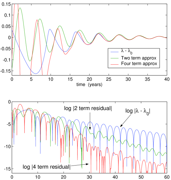
Figure 12: Higher order corrections in the asymptotic expansion

For both stable and unstable growth cycles there is always a spontaneous complex root pair $\nu_{2,3}$, as above, with a period typically of the order of a few years. This is the origin of the Great Moderation exhibited by the Keen Model. While by more abstract argument such a qualitative phenomenon may more easily be deduced, insofar as one wishes a precise determination of the period and growth rate, these values evidently cannot emerge from any more elementary analysis than that given here, which rests upon a particular balance of higher order terms. As $\Re(\nu_{2})>0$, this indicates a growing transient. But, as incorporated above, there is either a real offset of $\nu_{2}-\mu_{0}$ in the same exponential (as for $\lambda$) or else a separate term growing faster as $\mu_{0}$, against which background this growth loses ground, hence the effect is always one of relative decay.

It is the rare nonlinear ninth-order system that admits a general solution and, by means of that, access to a parametric understanding of all essential aspects of the system. It seems this is a peculiarity of debt-driven economic systems and the present elementary approach to determine a hierarchy of exponents should thus be borne in mind when considering other models of this sort.

References

- Bender and Orszag (1978) Bender, C., Orszag, S., 1978. Advanced mathematical methods for scientists and engineers, First Edition. McGraw-Hill.
- Cvitanović (1992) Cvitanović, P., 1992. Periodic orbit theory in classical and quantum mechanics. Chaos 2 (1), 1–4.
- Fontana (2000) Fontana, G., 2000. Post Keynsians and Circuitists on money and uncertainty: an attempt at generality. J. Post Keynesian Econ. 23 (1), 27–48.
- Grasselli and Costa Lima (2012) Grasselli, M., Costa Lima, B., 2012. An analysis of the Keen model for credit expansion, asset price bubbles and financial fragility. Mathematics and Financial EconomicsTo appear.
- Graziani (1990) Graziani, A., 1990. The theory of the monetary circuit. Economies et Societes 24 (6), 7–36.
- Hudson (2009) Hudson, M., 2009. A tax program for U.S. economic recovery. http://michael-hudson.com/2009/02/a-tax-program-for-u-s-economic-recovery.
- Hudson (2010) Hudson, M., 2010. From Marx to Goldman Sachs: The fictions of fictitious capital, and financialization of industry. Critique 38 (3), 419–444.
- Hudson (2012) Hudson, M., February 2012. The road to debt deflation, debt peonage, and neofeudalism. Working Paper 708, Levy Economics Institute of Bard College.
- Keen (1995) Keen, S., 1995. Finance and economic breakdown: Modeling Minsky’s ‘Financial Instability Hypothesis’. Journal of Post Keynesian Economics 17 (4), 607–635.
- Keen (2011a) Keen, S., 2011a. Are We “It” Yet? http://www.debtdeflation.com/blogs/2010/07/03/are-we-it-yet.
- Keen (2011b) Keen, S., 2011b. Debunking economics: The naked emperor dethroned, Second Edition. Zed Books.
- Keen (2011c) Keen, S., 2011c. Debunking macroeconomics. Economic Analysis & Policy 41 (3), 147–167.
- Keen (2012) Keen, S., 2012. A monetary Minsky model of the Great Moderation and the Great Recession. Journal Economic Behavior & OrganizationDoi:10.1016/j.jebo.2011.0.010, in press.
- Lerner (1970) Lerner, A., 1970. The economics of control, reprinting of First Edition. Augustus M. Kelley.
- Minsky (2008) Minsky, H., 2008. Stabilizing an unstable economy, Second Edition. McGraw-Hill.
- Schumpeter (1934) Schumpeter, J., 1934. The theory of economic development: An inquiry into profits, capital, credit, interest, and the business cycle. Vol. 46 of Harvard Economic Studies. Harvard University Press, Cambridge, translated from the German by Redvers Opie.