An approximate N³LO cross section for Higgs production in gluon fusion

Abstract

An approximate expression for the inclusive Higgs production cross section in gluon fusion at N³LO in QCD with finite top mass is presented. We argue that an accurate approximation can be constructed combining (and improving) the large- and small-$z$ behaviours of the partonic cross section, which are both known to all orders from soft-gluon (Sudakov) and high-energy (BFKL) resummations, respectively. For a $125$ GeV Higgs at LHC at $8$ TeV, we find an increase of about $6$–$13\%$ with respect to the NNLO inclusive cross section for the conventional scale $\mu_{\scriptscriptstyle\rm R}=m_{H}/2$, suggesting that higher order QCD corrections might be underestimated by presently available results. We also find a significant reduction of the scale uncertainty.

1 Introduction

In the aftermath of the discovery of the Higgs boson, the measurement of its properties is one of the main tasks of the LHC experiments. Accurate theoretical predictions play a fundamental role in such measurements. However, the cross section for Higgs production through gluon fusion (the dominant production channel) is affected by a very bad perturbative behavior. Indeed, QCD corrections to the process, known at NLO spira1 ; dawson ; spira2 and NNLO harlanderNNLO ; anastasiouNNLO ; ravindranNNLO ; Higgsfinite ; harlander1 ; harlander3 ; pak1 , give rise to very large $K$-factors, and only a mild reduction of the scale dependence. Therefore, the knowledge of the impact of yet higher order corrections is mandatory.

Although the computation of the N³LO correction (as a soft expansion and in the large $m_{t}$ limit) to the cross section is in progress anastasiouintegrals ; Hoschele:2012xc ; Anastasiou:2013srw ; Buehler:2013fha , in Ref. Ball:2013bra we have derived an approximate expression for it. Our approximation is based on combining a soft approximation and a high-energy approximation, taking into account the exact $m_{t}$ dependence. The consistency of the combination gives some constraints which turn out to improve significantly the accuracy and the reliability of the result.

In the following we briefly review the basic properties of our approximation, while we refer the Reader to Ref. Ball:2013bra for a detailed discussion, and we present some new unpublished results, namely we show our prediction for higher LHC energies and we discuss the impact of the virtually largest unknown contribution at order $\alpha_{s}^{3}$.

2 Combined soft and high-energy approximations

The inclusive Higgs production cross section is given as a sum over partons of convolutions of a parton luminosity $\mathscr{L}_{ij}(x,\mu_{\scriptscriptstyle\rm F}^{2})$ and a coefficient function $C_{ij}$,

$$\sigma(\tau,m_{H}^{2})=\tau\,\sigma_{0}(m_{H}^{2},\alpha_{s})\sum_{i,j=\{q,g\}}\int_{\tau}^{1}\frac{dz}{z}\,\mathscr{L}_{ij}\mathopen{}\mathclose{{}\left(\frac{\tau}{z},\mu_{\scriptscriptstyle\rm F}^{2}}\right)\\ \times C_{ij}\mathopen{}\mathclose{{}\left(z,\alpha_{s},\mu_{\scriptscriptstyle\rm R}^{2}/m_{H}^{2},\mu_{\scriptscriptstyle\rm F}^{2}/m_{H}^{2}}\right),$$ (1)

where $\alpha_{s}\equiv\alpha_{s}(\mu_{\scriptscriptstyle\rm R}^{2})$, $\sigma_{0}(m_{H}^{2},\alpha_{s})$ is the leading order partonic cross section, $\tau=m_{H}^{2}/s$ and $\mu_{\scriptscriptstyle\rm F}$, $\mu_{\scriptscriptstyle\rm R}$ are the factorization and renormalization scales. The sum over partons is dominated by $i=j=g$, the other channels giving a contribution of about $3\%$ of the total result at NNLO. Concentrating therefore on the $gg$ channel, and suppressing the subscripts and the dependence on the scales, we have the expansion

$$C(z,\alpha_{s})=\delta(1-z)+\alpha_{s}C^{(1)}(z)+\alpha_{s}^{2}C^{(2)}(z)+\alpha_{s}^{3}C^{(3)}(z)+\ldots$$ (2)

Currently, the NLO coefficient $C^{(1)}(z)$ is known exactly spira2 , while the NNLO coefficient $C^{(2)}(z)$ is known either in the large-$m_{t}$ effective theory harlanderNNLO ; anastasiouNNLO ; ravindranNNLO or as an expansion in powers of $m_{H}/m_{t}$ Higgsfinite ; harlander1 ; harlander3 ; pak1 .

In Ref. Ball:2013bra we have constructed an approximation to the N³LO coefficient based on the decomposition

$$C^{(3)}_{\rm approx}(z)=C_{\text{soft}}^{(3)}(z)+C_{\text{h.e.}}^{(3)}(z),$$ (3)

where $C_{\text{soft}}$ contains terms predicted by soft-gluon (Sudakov) resummation and reproduces the $z\to 1$ behavior, and $C_{\text{h.e.}}$ contains terms predicted by high-energy (BFKL) resummation and describes the $z\to 0$ limit. In $N$ space, where $N$ is the variable conjugate to $z$ by Mellin transformation, $C_{\text{soft}}^{(3)}(N)$ reproduces the logarithmic large $N$ behavior and $C_{\text{h.e.}}^{(3)}(N)$ the rightmost singularity in $N=1$. In principle, if all the singularities in the complex $N$ plane were known, it would be possible to reconstruct the function everywhere; in practice, the knowledge of the dominant singularities ($N=\infty$ and $N=1$) is sufficient to give a good approximation of the function in the physical region $\mathrm{Re}\>N>1$, the other singularities, placed at integer non-positive values of $N$, giving a subdominant contribution.

In the following we give some details on the construction of both approximations, with an emphasis on the improvements over the commonly used results, and we will demonstrate the reliability of the approximations by comparison to the first two known perturbative orders.

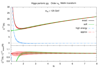
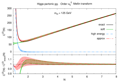
Figure 1: Comparison of the NLO (left) and NNLO (right) exact coefficient functions to their soft, high-energy and combined approximations.

2.1 Improved soft approximation

The largest contribution at the current and foreseeable future collider energies comes from the soft part. This is mainly due to the fact that the gluon-gluon luminosity, peaked at small $x$, enhances the contribution from the soft region of the partonic coefficient. This statement can be made quantitative in $N$ space, by means of a saddle point argument bfrsaddle , noticing that the region of $N$ contributing to the hadron-level cross section is localized about the position of the saddle point of the Mellin inversion integrand. For $m_{H}=125$ GeV and $\sqrt{s}=8$ TeV, the saddle point is at $N\sim 2$, a value at which the high-energy contribution is small (see Sect. 2.2).

On the other hand, the region $N\sim 2$ cannot be regarded as a large $N$ region, given that terms suppressed by one or more powers of $1/N$ with respect to the logarithmically growing soft terms, hereafter called subdominant, usually negligible at large $N$, give in general a sizable contribution at $N\sim 2$. Therefore, the quality of a soft approximation at the saddle point strictly depends on the control on such subdominant terms. In fact, some of these terms are under control to all orders in perturbation theory Kramer:1996iq , and their inclusion in a soft approximation leads to a significant improvement of the quality of the approximation itself.

Our soft approximation is constructed as follows. Starting from a resummed (all-order) soft expression in $N$ space, we expand it in powers of $\alpha_{s}$, obtaining a linear combination of powers of $\log N$. We then take the inverse Mellin transform, which is a linear combination of logarithms of the form

$$\frac{\log^{k}\log\frac{1}{z}}{\log\frac{1}{z}}$$ (4)

for integer values of $k$. We then apply the following two improvements:

• We use the exact logarithmic terms as originating from the kinematics of gluon emissions, which have the form

  $$\frac{\log^{k}\frac{1-z}{\sqrt{z}}}{1-z}.$$ (5)

  Usually the factor $\sqrt{z}$ is neglected in the soft limit, and in resummed expressions the Mellin transform of such terms, which is given by polygamma functions, is approximated with powers of $\log N$. This second approximation, in particular, is incompatible with the analytic structure of the coefficient function, since $\log N$ has a branch-cut for negative real $N$ while polygamma functions have just poles in integer non-positive values of $N$.

• We include for each emission the appropriate (leading) Altarelli-Parisi splitting kernel,

  $$p_{gg}(z)=\frac{A_{g}(z)}{1-z},\quad A_{g}(z)=\frac{C_{A}}{\pi}\frac{1-2z+3z^{2}-2z^{3}+z^{4}}{z}.$$ (6)

  Usually, $A_{g}(z)$ is approximated with $A_{g}(1)$, and only the divergent part of $p_{gg}$, $(1-z)^{-1}$, is kept. However, we point out (following an observation in Ref. Kramer:1996iq ) that the inclusion of subleading terms in $A_{g}(z)$ significantly improves the soft approximation. In fact, the exact expression of $A_{g}(z)$ would introduce a double counting with high-energy terms (because of the $z^{-1}$ term), and we therefore use an expansion of $A_{g}(z)$ about $z=1$ to order $1$ and $2$ (above $2$ there is no practical difference in the region $N\gtrsim 2$). The difference between these two results gives information on the size of the subdominant terms that are not included, and therefore provides a measure of the uncertainty associated with the soft approximation.

In Fig. 1 the NLO and NNLO coefficient functions $C^{(1)}(N)$ and $C^{(2)}(N)$ are shown together with their soft approximations. The two green curves (filled with a green band in between) represent the construction of the soft approximation described above, for the expansion of $A_{g}(z)$ to first and second order in $(1-z)$. It is clear from the plots that the soft approximation reproduces well the exact coefficient for $N\gtrsim 2$, the approximation obtained expanding to second order $A_{g}(z)$ (the lower green curve at large $N$) being closer to the exact result.

2.2 High-energy approximation

The leading pole in $N=1$ at each power of $\alpha_{s}$ is predicted to all orders by BFKL resummation Ball:2007ra ; abfquarks , and can be obtained from the all-order formula

$$C_{\text{ABF}}(N,\alpha_{s})=\sum_{\begin{subarray}{c}i_{1},i_{2}\geq 0\\ i_{1}+i_{2}>0\end{subarray}}c_{i_{1},i_{2}}\mathopen{}\mathclose{{}\left[\gamma_{+}^{i_{1}}(N,\alpha_{s})}\right]\mathopen{}\mathclose{{}\left[\gamma_{+}^{i_{2}}(N,\alpha_{s})}\right],$$ (7)

where $\gamma_{+}$ is the largest eigenvalue of the DGLAP singlet anomalous dimension matrix, the square brackets symbolize the inclusion of running coupling effects Ball:2007ra ; abfquarks , and $c_{i_{1},i_{2}}$ are numeric coefficients that have been computed to the first few orders in Refs. Higgsfinite ; marzaniPhD . Eq. (7) predicts correctly the coefficient of the highest order $N=1$ pole at each power of $\alpha_{s}$, provided the anomalous dimension is accurate at the same (leading logarithmic) level. However, for a consistent resummed result it is more convenient to use the resummed anomalous dimension, because the resummation changes the position of the leading pole. Since the resummed anomalous dimension vanishes in $N=2$ (momentum conservation) this implies, in turn, that $C_{\text{ABF}}(2,\alpha_{s})$ would vanish as well.

For our purpose, i.e. obtaining a high-energy approximation to the coefficient function at a finite perturbative order, we consider the expansion of Eq. (7):

$$C_{\text{ABF}}(N,\alpha_{s})=\sum_{n=1}^{\infty}\alpha_{s}^{n}C_{\text{ABF}}^{(n)}(N).$$ (8)

The computation of $C_{\text{ABF}}^{(3)}(N)$ requires the anomalous dimension $\gamma_{+}$ up to order $\alpha_{s}^{3}$. We could use the exact anomalous dimension, which is known; however, it grows logarithmically at large $N$, and this would interfere with the soft approximation, spoiling its accuracy. Therefore we adopt the following procedure:

• We take an expansion of the anomalous dimension about $N=1$ to NLL order (namely the largest and the next-to-largest pole at each order in $\alpha_{s}$). We stress that the final result, $C_{\text{ABF}}^{(n)}(N)$, is still accurate at LL only, though the NLL terms included in this way may (and do) improve the accuracy of the approximation.

• Since $C_{\text{ABF}}^{(n)}(N)$ constructed in this way still doesn’t vanish at large $N$, we subtract the large $N$ terms,

  $$C_{\text{ABF-sub}}^{(n)}(N)=C_{\text{ABF}}^{(n)}(N)-2C_{\text{ABF}}^{(n)}(N+1)+C_{\text{ABF}}^{(n)}(N+2),$$ (9)

  introducing spurious poles at integers $N\leq 0$, hereafter called subdominant, which are beyond our control. This subtraction corresponds to a $z$-space damping $(1-z)^{2}$.

• Finally, since the momentum conservation property of $C_{\text{ABF}}$ is lost in this procedure, we restore it by hand adding a subdominant term,

  $$C_{\text{h.e.}}^{(n)}(N)=C_{\text{ABF-sub}}^{(n)}(N)-\frac{4!\,k_{\rm mom}}{N(N+1)(N+2)},$$ (10)

  where $k_{\rm mom}$ must equal $C_{\text{ABF-sub}}^{(n)}(2)$. In order to estimate the impact of subdominant poles, we assign an arbitrary $5\%$ uncertainty to $k_{\rm mom}$, using $C_{\text{soft}}(2)$ as a reference:

  $$k_{\rm mom}=C_{\text{ABF-sub}}(2)\pm 0.05\times C_{\text{soft}}(2).$$ (11)

The results at NLO and NNLO are shown in Fig. 1. The high-energy part alone is accurate only very close to the singularity in $N=1$, while it vanishes fast for $N\gtrsim 2$. The combination $C_{\text{soft}}+C_{\text{h.e.}}$, red curves (corresponding to the two soft curves), is instead very accurate in the whole range $N>1$. The red band is the (linear) combination of the soft and high-energy uncertainties, and represents our final estimate of the error from neglected subdominant terms.

We conclude that our construction is robust and gives accurate approximations to the first two orders in perturbation theory. Arguing that this feature remains true at higher orders, we have constructed an approximate expression for the third order coefficient, Eq. (3). In the next Section we will use it to predict the N³LO cross section.

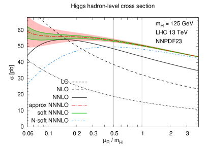
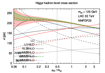
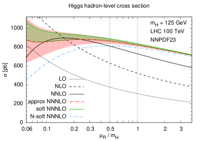
Figure 2: Dependence of the N³LO cross section on the renormalization scale $\mu_{\scriptscriptstyle\rm R}$, for $\mu_{\scriptscriptstyle\rm F}=m_{H}=125$ GeV and collider energy $8$ TeV (top-left), $13$ TeV (top-right), $33$ TeV (bottom-left) and $100$ TeV (bottom-right). The two standard choices of renormalization scale are shown as vertical lines.

3 Results

We present here the result for the production cross section of a Higgs boson with mass $m_{H}=125$ GeV at the LHC for several collider energies. Differently from Ref. Ball:2013bra , we use here the NNPDF2.3 pdf set Ball:2012cx , with $\alpha_{s}(m_{Z}^{2})=0.118$. Results are obtained with the code ggHiggs code .

In Fig. 2 we show the dependence of the cross section on the renormalization scale $\mu_{\scriptscriptstyle\rm R}$, keeping the factorization scale fixed $\mu_{\scriptscriptstyle\rm F}=m_{H}$ (in this way we capture the largest dependence at low collider energies, since the factorization scale dependence is very mild over a wide range Ball:2013bra ; Buehler:2013fha ). In addition to the exact (with exact $m_{t}$ dependence) LO, NLO and NNLO, we show our approximation for the N³LO cross section (red curve) with the estimated error from the unknown subdominant terms (red band) as described in Sect. 2. We observe that our prediction corresponds to an increase of the cross section which ranges from about $17\%$ to about $13\%$ for collider energies from $8$ TeV to $100$ TeV at the central scale $\mu_{\scriptscriptstyle\rm R}=m_{H}$, while the increase is lower at the scale $\mu_{\scriptscriptstyle\rm R}=m_{H}/2$, from about $11\%$ to about $7\%$ for the same energies.

To show the impact of the soft and high-energy terms separately, we also plot the approximation obtained considering the soft terms only (green lines and band). For instance, at $\sqrt{s}=13$ TeV (next LHC energy) the impact in our central prediction of the high-energy terms is minimal, since the red curve lies almost exactly in the middle of the soft green band. At higher collider energies, the high-energy terms become more relevant, consistently to the fact that at higher energies the saddle point moves to lower values bfrsaddle (about $N\sim 1.7$ at $\sqrt{s}=100$ TeV).

The plots show another curve denoted $N$-soft, which corresponds to a soft approximation as obtained if we do not apply the two improvements described in Sect. 2.1. Such a curve is conceptually identical to the result of Ref. MV , except some minor details. Therefore, the difference between our soft curves and the $N$-soft curve is entirely due to the improvements we have introduced. Such improvements turn out to predict a larger cross section, and give a flatter scale dependence in the region of low $\mu_{\scriptscriptstyle\rm R}$, where some sort of convergence of the perturbative expansion shows up.

We finally discuss the impact of unknown dominant terms. Indeed, the error band in our result accounts for subdominant (i.e., not fixed by the resummation formalism) unknown contributions, but in fact some dominant terms are unknown. As discussed in Sect. 2.2, the high-energy approximation is accurate only at LL level, but at order $\alpha_{s}^{3}$ also NLL and NNLL contribute. These contributions are definitely important close to $N=1$, but they are likely of the same order of subdominant terms at $N\sim 2$ (where the saddle point lies for $\sqrt{s}=8$ TeV), and are therefore already taken into account by our uncertainty band. On the other hand, at order $\alpha_{s}^{3}$ all the soft logarithmic terms are known, but the $\delta(1-z)$ coefficient, corresponding in $N$ space to a constant term, is unknown.

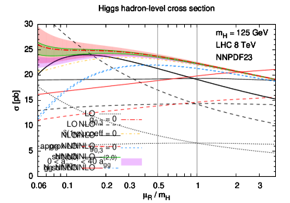
Figure 3: Same as Fig. 2 for $\sqrt{s}=8$ TeV, using different guesses for the unknown $\delta(1-z)$ term at order $\alpha_{s}^{3}$.

To investigate the impact of such unknown term, in Fig. 3 we show several possibilities:

• In our approximation we have kept as a default choice all the constant terms in $N$ space coming from the Mellin transform of the plus distributions, and we have set to zero all the others. According to the terminology introduced in Ref. Ball:2013bra , we have set $\bar{g}_{0,3}=0$.

• This choice is conceptually similar to omitting the coefficient of $\delta(1-z)$ at order $\alpha_{s}^{3}$, as suggested in Ref. MV .

• A third possibility, which would be adopted in a naive NNNLL resummation, would be to set to zero all the constant terms in $N$-space, $g_{0,3}=0$.

• Another possibility is to estimate the $\delta(1-z)$ coefficient from lower orders Buehler:2013fha . In the large $m_{t}$ effective theory, such coefficient factorizes into a Wilson coefficient and a “pointlike” expansion in powers of $\alpha_{s}/\pi$, whose coefficients have been called $a_{gg}^{(n,0)}$ in Ref. Buehler:2013fha . Up to order $\alpha_{s}^{2}$ such coefficients are well behaved, with $a_{gg}^{(1,0)}/a_{gg}^{(0,0)}\sim 10$ and $a_{gg}^{(2,0)}/a_{gg}^{(1,0)}\sim 1.4$, and it then appears reasonable to estimate $0<a_{gg}^{(3,0)}/a_{gg}^{(2,0)}<40$, as proposed in Ref. Buehler:2013fha .

Except the option $g_{0,3}=0$, which looks unreasonable in the light of the large coefficients of the perturbative expansion of $g_{0}(\alpha_{s})$ Ball:2013bra , all the other options are quite close each other, and give an uncertainty comparable to the one from subdominant terms. It is interesting to observe that our default option predicts the largest cross section, while the smaller (reasonable) prediction is obtained setting to zero the coefficient of the $\delta(1-z)$ term, which would decrease the size of the N³LO contribution from about $11\%$ to about $8\%$ at $\mu_{\scriptscriptstyle\rm R}=m_{H}/2$. Anyway, the difference among these predictions can only set the size of the uncertainty associated with the unknown coefficient, though only the computation of such coefficient (even in the large $m_{t}$ effective theory) can solve the ambiguity.

4 Conclusions

We have constructed an approximation to the Higgs production cross section combining and improving soft and high-energy behaviors. At the known orders, such approximation accurately reproduces the exact result within the estimated error coming from subdominant terms. We have then used it to predict the N³LO cross section. The largest uncertainty on our approximation comes from the unknown dominant term proportional to $\delta(1-z)$, whose impact has been studied in some detail, and whose uncertainty can only be fixed by its computation. Taking into account all the uncertainties, we can reasonably conclude that the N³LO correction amounts to a $6$–$13\%$ increase over the NNLO at the conventional scale $\mu_{\scriptscriptstyle\rm R}=m_{H}/2$ for $\sqrt{s}=8$ TeV. We also note that the scale uncertainty in the conventional range $m_{H}/4<\mu_{\scriptscriptstyle\rm R}<m_{H}$ is reduced from $4.1$ pb at NNLO to $2.3$ pb at N³LO, which is rather larger than the uncertainty on our approximation. This proves that our result, though approximate, reduces the uncertainty on the Higgs cross section, and provides therefore a step forward in the Higgs precision phenomenology task.

References

- (1) A. Djouadi, M. Spira and P. M. Zerwas, Phys. Lett. B 264 (1991) 440.
- (2) S. Dawson, Nucl. Phys. B 359 (1991) 283.
- (3) M. Spira, A. Djouadi, D. Graudenz and P. M. Zerwas, Nucl. Phys. B 453 (1995) 17 [hep-ph/9504378].
- (4) R. V. Harlander and W. B. Kilgore, Phys. Rev. Lett. 88 (2002) 201801 [hep-ph/0201206].
- (5) C. Anastasiou and K. Melnikov, Nucl. Phys. B 646 (2002) 220 [hep-ph/0207004].
- (6) V. Ravindran, J. Smith and W. L. van Neerven, Nucl. Phys. B 665 (2003) 325 [hep-ph/0302135].
- (7) S. Marzani, R. D. Ball, V. Del Duca, S. Forte and A. Vicini, Nucl. Phys. B 800 (2008) 127 [arXiv:0801.2544 [hep-ph]].
- (8) R. V. Harlander and K. J. Ozeren, Phys. Lett. B 679 (2009) 467 [arXiv:0907.2997 [hep-ph]]; JHEP 0911 (2009) 088 [arXiv:0909.3420 [hep-ph]].
- (9) R. V. Harlander, H. Mantler, S. Marzani and K. J. Ozeren, Eur. Phys. J. C 66 (2010) 359 [arXiv:0912.2104 [hep-ph]].
- (10) A. Pak, M. Rogal and M. Steinhauser, Phys. Lett. B 679 (2009) 473 [arXiv:0907.2998 [hep-ph]]; JHEP 1002 (2010) 025 [arXiv:0911.4662 [hep-ph]].
- (11) C. Anastasiou, S. Buehler, C. Duhr and F. Herzog, arXiv:1208.3130 [hep-ph].
- (12) M. Hoschele, J. Hoff, A. Pak, M. Steinhauser and T. Ueda, arXiv:1211.6559 [hep-ph].
- (13) C. Anastasiou, C. Duhr, F. Dulat and B. Mistlberger, arXiv:1302.4379 [hep-ph].
- (14) S. Buehler and A. Lazopoulos, arXiv:1306.2223 [hep-ph].
- (15) R. D. Ball, M. Bonvini, S. Forte, S. Marzani and G. Ridolfi, arXiv:1303.3590 [hep-ph].
- (16) M. Bonvini, S. Forte and G. Ridolfi, Phys. Rev. Lett. 109 (2012) 102002 [arXiv:1204.5473 [hep-ph]].
- (17) M. Kramer, E. Laenen and M. Spira, Nucl. Phys. B 511 (1998) 523 [hep-ph/9611272].
- (18) R. D. Ball, Nucl. Phys. B 796 (2008) 137 [arXiv:0708.1277 [hep-ph]].
- (19) G. Altarelli, R. D. Ball and S. Forte, Nucl. Phys. B 799 (2008) 199 [arXiv:0802.0032 [hep-ph]].
- (20) S. Marzani, PhD thesis, The University of Edinburgh (2008).
- (21) R. D. Ball, V. Bertone, S. Carrazza, C. S. Deans, L. Del Debbio, S. Forte, A. Guffanti and N. P. Hartland et al., Nucl. Phys. B 867 (2013) 244 [arXiv:1207.1303 [hep-ph]].
- (22) http://www.ge.infn.it/bonvini/higgs/
- (23) S. Moch and A. Vogt, Phys. Lett. B 631 (2005) 48 [hep-ph/0508265].