Finding the Rashba-type spin-splitting from interband scattering in quasiparticle interference maps

Abstract

We have studied the BiCu₂/Cu(111) surface alloy using low-temperature scanning tunneling microscopy and spectroscopy. We observed standing waves caused by scattering off defects and step edges. Different from previous studies on similar Rashba-type surfaces, we identified multiple scattering vectors that originate from various intraband as well as interband scattering processes. A detailed energy-dependent analysis of the standing-wave patterns enables a quantitative determination of band dispersions, including the Rashba splitting. The results are in good agreement with ARPES data and demonstrate the usefulness of this strategy to determine the band structure of Rashba systems. The lack of other possible scattering channels will be discussed in terms of spin conservation and hybridization effects. The results open new possibilities to study spin-dependent scattering on complex spin-orbit coupled surfaces.

The Bychkov-Rashba effect lifts the spin-degeneracy at surfaces and interfaces in environments with a sizeable spin-orbit interaction Bychkov and Rashba (1984). Up to date, many different systems with various kinds of splitting strengths have been identified LaShell et al. (1996); Koroteev et al. (2004); Ast et al. (2007a). Its characteristic band dispersion is readily recognizable in angular resolved photoemission experiments and generally good agreement is achieved between theoretical calculations and experimentally observed electronic structures Petersen and Hedegård (2000); Ast et al. (2007a); Bihlmayer et al. (2007); Gierz et al. (2010); Moreschini et al. (2009); Bentmann et al. (2009, 2011); Ünal et al. (2012). The Rashba parameter can also be extracted from the local density of states measured by scanning tunneling spectroscopy (STS) Ast et al. (2007b). However, identifying the Rashba-type spin-splitting from quasiparticle interference (QPI) patterns measured by STS remains elusive. The reason for this is the defined spin-polarization for each singly degenerate state resulting in forbidden backscattering. As a consequence, the Rashba signature is suppressed in QPI patterns of isotropic band structures, making the pattern look like it originates from a spin-degenerate state Petersen and Hedegård (2000). In highly anisotropic surface states, e.g. Bi(110) Pascual et al. (2004) or Bi_1-xSb_x(111) Roushan et al. (2009), the “spin-selection rule” strongly reduces the set of possible momentum transfers, so that the presence of a Rashba-type spin-splitting can be observed qualitatively. QPI patterns from multiple scattering events can also give a qualitative difference between spin-split states and spin-degenerate states Walls and Heller (2007). However, a quantitative statement about the strength of the spin-splitting from the analysis of QPI patterns has not been reported so far.

Here, we show that it is possible to extract the Rashba parameter from interband scattering events in QPI patterns using scanning tunneling microscopy (STM) and STS. For this proof of principle, we choose the well-known system BiCu₂/Cu(111). Differential conductance maps at different energies reveal standing-wave patterns due to scattering at defects and step edges. A careful Fourier-transform (FT) analysis reveals several scattering vectors, which can be related to intraband transitions within the first $sp_{z}$-type surface state, intraband transitions within the second ($p_{xy}$) surface state, and interband transitions between the first and second surface state. A detailed data set at several energies is used to recover the dispersion relations of both surface states, including the Rashba-type spin-splitting.

The experiments were performed in ultrahigh vacuum (UHV) using a commercial low-temperature STM (Createc LT-STM) operated at $T=6\,\text{K}$. A Cu(111) single-crystal substrate was first cleaned by standard sputter-annealing procedures. The BiCu₂ surface alloy was then grown by evaporating one third of a monolayer of Bi onto the Cu substrate from a Knudsen cell. During and for 10 minutes after the deposition, the substrate was held at about 390 K. The sample was then transferred in situ into the cryogenic STM. Topography images were taken in constant-current mode. STS was performed by measuring the differential conductance $dI/dV$ as a function of the sample bias $V$ by standard lock-in techniques ($V_{\text{mod}}=1-20\,\text{mV}$ (rms), frequency $768.3\,\text{Hz}$) under open-feedback conditions. $dI/dV$ maps at various energies were taken in constant-current as well as constant-height mode using $V_{\text{mod}}=20\,\text{mV}$. The maps were then Fourier-transformed and analyzed using a commercial image analysis software (Image Metrology SPIP).

Figure 1: (Color online) STM topography of BiCu₂/Cu(111). (a) The overview image shows a smooth surface with an antiphase boundary and a few point defects. Due to the low sample bias (1 mV, 100 pA), standing waves can be observed. (b) Close-up view of the $\sqrt{3}\times\sqrt{3}$ structure (1 mV, 63 nA). Bi atoms appear bright (cf. structural model on top right). (c) A close-up view of the antiphase boundary. (d,e) Zoom images of the top left and bottom left point defects in (a) show small topographical differences.

Figure 1 shows STM images of the surface alloy. We found large atomically smooth surfaces with typical sizes of about $1000\times 1000$ Ų, limited by step edges and antiphase boundaries. Fig. 1a shows an overview of a large terrace. A close-up view (b) of the surface reveals the well-known BiCu₂ surface with a $\sqrt{3}\times\sqrt{3}$ structure and a lattice constant of 4.42 Å (cf. structural model superimposed in (b)) Kaminski et al. (2005). Bi atoms appear as bright protrusions, while the surrounding Cu atoms cannot be resolved atomically Ast et al. (2007b); Gierz et al. (2010). On the right-hand side, the overview image shows a trench. As can be seen in (c), this feature corresponds to an antiphase boundary of two superstructures on the left and right-hand sides, respectively. In addition, point defects can be observed, which are at positions where a Bi atom should be located. We assume that they are sites where a Cu atom has not been replaced by a Bi atom within the surface layer. We have observed two types of point scatterers that appear slightly different in topography images at low bias (d and e). While the reason is unknown, both show qualitatively identical scattering behavior (cf. Fig. 2) and will therefore be treated as being the same. The average defect density is less than $1/1000^{\text{th}}$ monolayer ($\approx 9\cdot 10^{-5}\text{\AA}^{-2}$, i.e., defect separation $\approx 120$ Å). As we will discuss later, this corresponds to a very good sample quality.

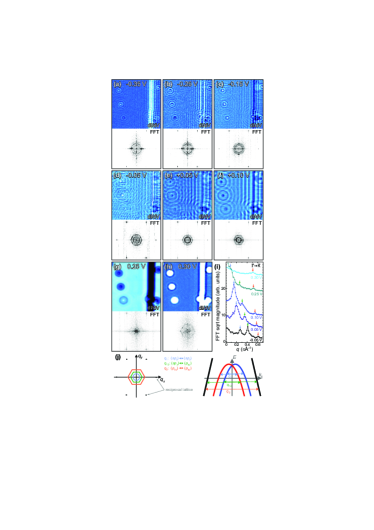
Figure 2: (Color online) FT-STS analysis of BiCu₂/Cu(111). (a-h) $dI/dV$ maps and corresponding FT images at different sample voltages. (i) FT cross sections along a $\overline{\Gamma}\overline{\text{K}}$ direction show the bias-dependent trend of the scattering features. (j) Schematic representation of the (up to) four features visible in the FT images and proposed assignments deduced from the band structure.

The topography image in Fig. 1a already shows standing waves on the surface: a planar wave front is scattered off the antiphase boundary, and the point defects are surrounded by circular waves. As is well-known, the energy-dependent wavelengths of these standing waves are directly connected to the dispersion relation of the surface bands Crommie et al. (1993); Hasegawa and Avouris (1993). To enable a thorough analysis of the underlying scattering processes, we have used the FT-STS method at various energies Sprunger et al. (1997). Fig. 2 summarizes some of the acquired $dI/dV$ maps and corresponding 2D-Fourier transformations . Interestingly, the maps in Fig. 2 undoubtedly show that the standing-wave pattern is caused by more than one wavelength.

In the FT images, up to four features can be identified that are schematically depicted in Fig. 2j. The strongest intensity is found in six spots with hexagonal symmetry (black dots in (j); they reflect the reciprocal lattice of the $\sqrt{3}\times\sqrt{3}$ surface reconstruction and allow us to identify the $\overline{\Gamma}\overline{\text{M}}$ directions at angles 0^∘ (horizontal axis), 60^∘ and 120^∘, respectively, while the $\overline{\Gamma}\overline{\text{K}}$ directions are found at 30^∘, 90^∘, and 150^∘. The second strongest FT signal is a small circular ring (light blue circle in (j)) whose radius decreases with increasing sample bias. At $E-E_{F}=0.25$ eV (g), this feature is still visible as a narrow signal in the center of the FT image , but disappears above 0.25 eV (h). In addition, a second ring is clearly visible that has a hexagonal shape (green in (j)). This feature also becomes smaller as we go from $-0.3$ eV to $0.25$ eV and vanishes at higher energies (g,h). The final feature is a faint third ring that also has hexagonal shape (orange in (j)). Although the intensity is rather weak, a careful analysis via cross sections of the FT images (cf. orange markers in Fig. 2i) allows a clear determination of this scattering feature between $-0.25$ eV and $0.5$ eV.

A comparison of the distinct energy and angular dependence of the three scattering rings with band-structure calculations and ARPES measurements permits an unambiguous assignment of the features to specific scattering transitions in the band structure. The smallest (light blue) feature is isotropic and dominates the FT images up to 0.25 eV but suddenly vanishes for higher energies (Fig. 2i). This is the expected behavior for scattering within the first $sp_{z}$-type surface state Moreschini et al. (2009); Bentmann et al. (2009). As schematically shown in Fig. 2j, this band is Rashba-split: for any $E(k_{\parallel})$ plane through the $\overline{\Gamma}$ point, two parabolas of opposite spin exist that are shifted away from the $\overline{\Gamma}$-point by a wave-vector offset $k_{0}$. During a scattering event, the spin is conserved Petersen and Hedegård (2000); Pascual et al. (2004); Hirayama et al. (2011). Therefore, $sp_{z}$-intraband scattering only occurs between the branches of the same spin, leading to only one possible scattering vector $q_{1}$, as depicted in Fig. 2j. We note that previous studies tend to interpret the scattering vector $q$ as identical to the wave vector $k_{\parallel}$ in the energy dispersion through the relation $q/2=k_{\parallel}$ Crommie et al. (1993); Hasegawa and Avouris (1993); Hirayama et al. (2011). This assignment is valid whenever a dispersion is symmetric around $\overline{\Gamma}$ Sprunger et al. (1997); Pascual et al. (2001); Schouteden et al. (2009). For the Rashba-split parabolas, the scattering can only give information on the effective mass and maximum of the band, but information on the wave vector offset $k_{0}$ in $k_{\parallel}$ direction (i.e., the Rashba splitting) is lost Petersen and Hedegård (2000).

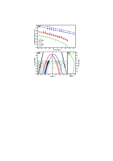
Figure 3: (Color online) Analysis of scattering channels and corresponding electronic structure. (a) Energy-dependence of $q_{1}$, $q_{2}$, and $q_{12}$ for $\overline{\Gamma}\overline{M}$ and $\overline{\Gamma}\overline{K}$ directions, respectively. Solid lines are fits to the data. (b) Band dispersions along $\overline{\Gamma}\overline{M}$ (solid lines) as determined from the fit. The points are experimentally derived $k$ values calculated from the $q_{i}$ vectors as indicated by the arrows (cf. Fig. 2j). For direct comparison, an ARPES result of the band dispersion is also shown (reproduced from Ref. Bentmann et al., 2009). (c) The STS spectrum exhibits a peak at 0.25 eV above $E_{F}$ that corresponds to the $sp_{z}$-band maximum, in agreement with the fit in (b).

In order to identify the outer (orange) scattering ring, its distinct hexagonal anisotropy can be compared to ARPES and DFT results Moreschini et al. (2009); Bentmann et al. (2009). A hexagonally shaped constant-energy surface is expected for the second surface band exhibiting $p_{xy}$ character. The wave vector $k_{\parallel}$ is larger along $\overline{\Gamma}\overline{\text{M}}$ compared to the $\overline{\Gamma}\overline{\text{K}}$ direction in accordance with our observed anisotropy. Also, the projected bulk-band edge, which is folded back due to the surface reconstruction, exhibits a hexagonal shape close to $\overline{\Gamma}$ Moreschini et al. (2009); Bentmann et al. (2009); Ünal et al. (2012). Here, however, the maximum wave vector is along $\overline{\Gamma}\overline{\text{K}}$. Hence, we can rule out transitions from or to bulk states. In fact, we find that the magnitude of the scattering vector is in very good agreement with the expected value for intraband scattering within the second surface state ($q_{2}$ in Fig. 2j). This also explains, why we can observe this feature in $dI/dV$ maps far beyond 0.25 eV (g-i). Within the energy range presented here, this band is spin-degenerate and symmetric around $\overline{\Gamma}$. Thus, we can directly deduce the dispersion relation via $k_{\parallel}(p_{xy})=q_{2}/2$.

The anisotropy of the middle (green) ring seen in the FT images is identical to the shape of the outer ring associated with $q_{2}$. Further, as the feature vanishes above 0.25 eV, the transition likely also involves the $sp_{z}$-band. Ruling out scattering channels that involve bulk states, the only possibility for this transition to occur is due to interband scattering between the $p_{xy}$- and $sp_{z}$-surface states. As the latter is Rashba-split, two different transitions can in principle be expected involving either the inner or the outer branch of the $sp_{z}$-band. A comparison of the magnitude reveals that our feature corresponds to scattering from (or to) the inner branch (denoted $q_{12}$ in Fig. 2j). Surprisingly, we have not found any indication for scattering between the the $p_{xy}$-band and the outer $sp_{z}$-branch (cf. discussion below).

Fig. 3a summarizes the energy dependence of the magnitude of all three scattering processes $q_{1}$, $q_{2}$, and $q_{12}$ along $\overline{\Gamma}\overline{\text{M}}$ and $\overline{\Gamma}\overline{\text{K}}$ as determined from the FT-STS data. In order to determine the band structure parameters from this data set, we assume a parabolic dispersion with a Rashba-type spin-splitting for the $sp_{z}$-band as well as a spin-degenerate linear dispersion for the $p_{xy}$-band. The linear dispersion is justified because in the relevant energy interval the band is located between the high-symmetry points in the vicinity of the inflection point, so that the band curvature can be neglected. Solving for the wave vector, the dispersion is $k(E)=\mu[2m^{*}(E-E_{0})/\hbar^{2}]^{1/2}+\lambda k_{0}$ with $\mu,\,\lambda=\pm 1$, where $\mu$ denotes the parabola branch and $\lambda$ denotes the Rashba branch Moreschini et al. (2009); Mirhosseini et al. (2009); Bentmann et al. (2009, 2011); Ünal et al. (2012). Here, $m^{*}$ is the effective mass and $E_{0}$ is the energy offset of the $sp_{z}$-band. Combining the intraband transitions $q_{1}$ and $q_{2}$ with the interband transition $q_{12}$, we can extract the wave vector offset determining the Rashba-type spin-splitting: $k_{0}=(q_{1}+q_{2})/2-q_{12}$. In order to decrease uncertainties of the fit procedure, we have simultaneously fit all three scattering vectors in both $\overline{\Gamma}\overline{\text{M}}$ and $\overline{\Gamma}\overline{\text{K}}$ directions (i.e., six data sets) using the same fit parameters (seven fit parameters: four describing the $p_{xy}$-band in $\overline{\Gamma}\overline{\text{M}}$ and $\overline{\Gamma}\overline{\text{K}}$ as well as $m^{*}$, $E_{0}$, and $k_{0}$). The solid lines in Fig. 3a are the resulting fit curves. Overall, we find very good agreement between the raw data and the fit. Table 1 summarizes the corresponding fit parameters in comparison with literature values. Using these values, we can plot the dispersion relations of the $p_{xy}$-band as well as the Rashba-split $sp_{z}$-band. The result is shown in Fig. 3b. The fit parameters and the extracted band dispersions agree well with other published data (see Table 1), despite the simplicity of the model used in this analysis. This demonstrates that we are able to fully recover the surface bands of this Rashba system, including the Rashba splitting $k_{0}$, the Rashba parameter $\alpha_{R}=\hbar^{2}k_{0}/m^{*}$, and the Rashba energy $E_{R}=\hbar^{2}k_{0}^{2}/2m^{*}$.

We find a slightly higher band maximum $E_{0}$ compared to previous studies. This is also confirmed by local STS spectra in Fig. 3c, where the band maximum appears as an asymmetric sharp peak at about 250 meV due to a singularity in the density of states Ast et al. (2007b); Wegner et al. (2006). We note that on other samples with higher local defect concentrations, we found reduced values for $E_{0}$. Moreover, confinement effects were evident on narrow terraces: as expected for a downward dispersing band, the peak in STS spectra was shifted to lower energies, roughly following an $L^{-2}$ dependence (where $L$ is the terrace width). As photoemission experiments probe large sample areas, we suggest that the previously reported smaller $E_{0}$ values may be a consequence of small terraces and/or reduced sample quality.

The magnitude of $m^{*}$ in our study is a bit smaller than reported before. However, our simple fit model merely considers a parabolic shape of the $sp_{z}$-band. While this is a good assumption for energies above $-0.2$ eV, ARPES measurements found a significant deviation for the outer branches: due to strong hybridization with bulk states below $-0.2$ eV, the dispersion bends down and exhibits a much steeper slope Moreschini et al. (2009); Bentmann et al. (2009). In our model we only use one average effective mass, therefore we expect it to be smaller.

Table 1: Results of parameters for the Rashba-split $sp_{z}$-type surface state of this work (FT-STS) compared to values reported in the literature.

	$m^{*}$ ($m_{e}$)	$E_{0}\,(\text{eV})$	$k_{0}\,(\text{\AA}^{-1})$	$\alpha_{R}\,(\text{eV{\AA}})$	$E_{R}\,(\text{eV})$
FT-STS	$-0.25(2)$	$0.25(1)$	$0.04(1)$	$1.2(3)$	$0.02(1)$
Ref. Moreschini et al.,2009	$-0.27$	$0.23$	$0.03$	$1.0$	$0.015$
Ref. Bentmann et al.,2009	$-0.30$	$0.231$	$0.032$	$0.82$	$0.013$
Ref. Ünal et al.,2012	$-0.37$	$0.23$	$0.04$	$0.83$	$0.020$

In agreement with previous observations on Bi surfaces and alloys, we found that the spin is conserved during the scattering process Petersen and Hedegård (2000); Pascual et al. (2004); Hirayama et al. (2011). As a result, we only observe scattering from the outer to the inner branch of the $sp_{z}$-band and vice versa ($q_{1}$). The $p_{xy}$-band is spin-degenerate in the energy region considered here Bentmann et al. (2009); Mirhosseini et al. (2009); Bentmann et al. (2011). Therefore, we were able to observe intraband scattering ($q_{2}$) as well as interband scattering to the inner branch of the $sp_{z}$-band ($q_{12}$). However, it is surprising at a first glance that we have not observed a scattering process involving the $p_{xy}$-band and the outer branch of the $sp_{z}$-band. While this transition is not forbidden per se, a bad wave-function overlap between initial and final state may lead to a vanishing scattering amplitude. Interestingly, ARPES and DFT results show that the inner and outer $sp_{z}$-branches behave very differently Moreschini et al. (2009); Bentmann et al. (2009): when crossing the bulk-band edge, the outer branch strongly hybridizes with the bulk states. This is obvious from the broadening, the loss of spectral density and the sudden deviation of the dispersion from the parabolic shape. On the other hand, the inner branch is barely influenced by bulk bands, as is the $p_{xy}$-band, indicating weak hybridization for these states. While further investigations are required, preliminary model calculations support the possibility that a reduced orbital overlap between the outer $sp_{z}$-branch and the $p_{xy}$-band combined with a large magnitude of the scattering vector can lead to a significantly reduced scattering amplitude that can be hidden in the background noise of our FT-STS data Krüger .

In conclusion, we have studied the QPI patterns in $dI/dV$ maps of the 2D-band structure in the BiCu₂/Cu(111) surface alloy using STS. While the scattering vectors from intraband scattering in the spin-split $sp_{z}$-band do not carry any information about the Rashba-type spin-splitting, a combination of intraband and interband scattering vectors from the $sp_{z}$-band and the spin-degenerate $p_{xy}$-band readily reveals the wave vector offset $k_{0}$ of the Rashba-type spin-splitting. Concerning topological insulators (TIs), the Rashba constant is ill-defined in these systems due to the different band topology. Nevertheless, our results show that additional scattering channels relax the condition of “forbidden backscattering”, which also applies for the TIs. This means that a TI can only feature forbidden backscattering if there is exactly one singly degenerate band crossing the Fermi level. Our results present a nice experimental proof of principle that the information about the Rashba-type spin-splitting is contained in QPI patterns and can be extracted when considering interband scattering. In this respect, the BiCu₂/Cu(111) surface alloy as well as other similar surface alloys can be used as excellent model systems to study the effects of spin-dependent scattering from, e.g., magnetic or non-magnetic adsorbates, multiple scattering events as well as confinement effects from smaller terraces or islands.