Extended Subspace Error Localization for Rate-Adaptive Distributed Source Coding

Abstract

A subspace-based approach for rate-adaptive distributed source coding (DSC) based on discrete Fourier transform (DFT) codes is developed. Punctured DFT codes can be used to implement rate-adaptive source coding, however they perform poorly after even moderate puncturing since the performance of the subspace error localization degrades severely. The proposed subspace-based error localization extends and improves the existing one, based on additional syndrome, and is naturally suitable for rate-adaptive distributed source coding architecture.

I Introduction

The ideas of coding theory can be described within the setting of signal processing by using a class of real (or complex) Bose-Chaudhuri-Hocquenghem (BCH) codes [1] known as the discrete Fourier transform codes. DFT codes find applications in different areas including wireless communications [2], joint source-channel coding [3], and distributed source coding [4]. Looking from a frame theory perspective, these codes are used to provide robustness to erasure in wireless networks [5, 6, 7].

When error correction is required [2, 3, 4], error localization is a crucial step of the decoding algorithm of DFT codes. Error localization in BCH-DFT codes can be done by extending that of binary BCH codes to the real field [1]. Rath and Guillemot [8] used subspace-based error localization and showed that it outperforms the coding-theoretic approach; the improvement is achieved by mitigating the effect of the quantization error by involving as many syndrome samples as possible. The authors recently employed DFT codes for lossy DSC [4] and adopted subspace error localization in this context [9]. This approach to DSC exploits the correlation between the sources in the analog domain and it is promising in delay-sensitive applications. The performance of the system, like other DSC systems, degrades when the correlation between the sources is unstable. Although puncturing can be used for rate-adaption, it severely affects the error localization and substantially increases the end-to-end distortion.

The primary contribution of this paper is to develop rate-adaptive distributed source codes based on DFT codes. To do so, we extend and improve the subspace error localization of DFT codes and adapt it both to the parity- and syndrome-based DSC. The extended subspace error localization is applicable to other codes based on orthogonal transform matrices such as the discrete cosine transform (DCT) and discrete sine transform (DST) codes, as the subspace approach is [10].

Rate-adaptation for the parity approach is developed only for real DFT codes of rate $0.5$. However, the syndrome approach is for any real or complex code; the encoder transmits a short syndrome based on an $(n,k)$ code and augments it with additional samples if decoding failure is fed back. The algorithm is incremental so that there is no need to re-encode the sources when more syndrome is requested.

The paper is organized as follows. After a brief review of DFT codes in Section II, we discuss how the subspace error localization outperforms the coding-theoretic approach and introduce the extended subspace decoding in Section III. We explain the rate-adaptive DSC system in Section IV. Numerical results in Section V confirm the merit of the proposed error localization. This is followed by conclusion in Section VI.

II DFT Codes

The generator matrix of an $(n,k)$ DFT code [11], in general, consists of any $k$ columns of the inverse DFT (IDFT) matrix of order $n$; the remaining $n-k$ columns of this matrix are used to build the parity-check matrix $H$. These codes are a family of cyclic codes over the complex field. Thus, their codewords satisfy certain spectral properties in the frequency domain [12]. Within the class of DFT codes, there are BCH codes in the complex and real fields. Each codeword of an $(n,k)$ BCH-DFT code has $d\triangleq n-k$ cyclically adjacent zeros in the frequency domain. They are maximum distance separable codes with minimum Hamming distance $d_{\min}=d+1$. They are, hence, capable of correcting up to $t=\lfloor\frac{d}{2}\rfloor$ errors.

We consider real BCH-DFT codes whose generator matrix, for an $(n,k)$ code, is defined by [13, 3]

$$G=\sqrt{\frac{n}{k}}W_{n}^{H}\Sigma W_{k},$$ (1)

where $W_{n}$ and $W_{k}$ are the DFT matrices of size $n$ and $k$, and

$$\Sigma=\left(\begin{array}[]{ccccccc}I_{\alpha}&\bm{0}\\ \bm{0}&\bm{0}\\ \bm{0}&I_{\beta}\\ \end{array}\right)$$ (5)

is an $n\times k$ matrix with $\alpha=\lceil\frac{n}{2}\rceil-\lfloor\frac{n-k}{2}\rfloor$ and $\alpha+\beta=k$.

The generator matrix of a complex BCH-DFT code can be achieved by removing $W_{k}$ from (1); we can also remove the constraint on $\alpha$. Although we focus on the real BCH-DFT codes, the results we present in this paper are valid for the complex codes as well. In the rest of this paper, for brevity, BCH-DFT codes will be referred to as DFT codes.

III Error Localization in DFT codes

Let $\bm{r}=\bm{c}+\bm{e}$ be a noisy version of codeword $\bm{c}$ generated by a DFT code and suppose that the error vector $\bm{e}$ has $\nu\leq t$ nonzero elements. Let $i_{1},\ldots,i_{\nu}$ and $e_{i_{1}},\ldots,e_{i_{\nu}}$, respectively, denote the locations and magnitudes of the nonzero elements. The decoding algorithm in DFT codes is composed of three main steps [1]: error detection (to determine $\nu$), error localization (to find $i_{1},\ldots,i_{\nu}$), and error calculation (to calculate $e_{i_{1}},\ldots,e_{i_{\nu}}$). This section is focused on the error localization. Thus, we assume that the number of errors $\nu$ is known at the decoder.

The syndrome of $\bm{e}$, a key for the decoding algorithm, is computed as

$$\bm{s}=H\bm{r}=H(\bm{c}+\bm{e})=H\bm{e},$$ (6)

where $\bm{s}=[s_{1},\,s_{2},\ldots,s_{d}]^{T}$ is a complex vector with

$$s_{m}=\frac{1}{\sqrt{n}}\sum_{p=1}^{\nu}e_{i_{p}}X_{p}^{\alpha-1+m},\quad m=1,\ldots,d,$$ (7)

in which $\alpha$ is defined in (5) and $X_{p}=e^{\frac{j2\pi i_{p}}{n}}$, $p=1,\ldots,\nu.$

III-A Coding-Theoretic and Subspace Approaches

The classical approach to the error localization is to identify an error locator polynomial whose roots correspond to error locations. The error locator polynomial is defined as

$$\Lambda(x)=\prod_{\begin{subarray}{c}i=1\end{subarray}}^{\nu}(1-xX_{i})=1+\Lambda_{1}x+\cdots+\Lambda_{\nu}x^{\nu},$$ (8)

and its roots $X_{1}^{-1},\ldots,X_{\nu}^{-1}$ correspond to the error locations $i_{p},p\in[1,\ldots,\nu]$, as $X_{p}^{-1}=\omega^{i_{p}}$ where $\omega=e^{-j\frac{2\pi}{n}}$. The coefficients $\Lambda_{1},\ldots,\Lambda_{\nu}$ can be found by solving the following set of consistent equations [1]

$$s_{j}\Lambda_{\nu}+s_{j+1}\Lambda_{\nu-1}+\cdots+s_{j+\nu-1}\Lambda_{1}=-s_{j+\nu},$$ (9)

for $j=1,\ldots,d-\nu$. To put it differently, as the IDFT of $\bm{\Lambda}_{n}=[1,\Lambda_{1},\ldots,\Lambda_{\nu},\bm{0}_{1\times(n-\nu-1)}]^{T}$ becomes zero at the error locations, the circular convolution of $\bm{\Lambda}_{n}$ with the DFT of the error vector is a zero vector [1, 8].

An alternative approach is to use the subspace methods for error localization [8]. The error-locator matrix of order $m$, whose columns are the error-locator vectors of order $m$, is a Vandermonde matrix defined as

$$V_{m}=\left[\begin{array}[]{cccc}1&1&\ldots&1\\ X_{1}&X_{2}&\ldots&X_{\nu}\\ \vdots&\vdots&\ddots&\vdots\\ X_{1}^{m-1}&X_{2}^{m-1}&\ldots&X_{\nu}^{m-1}\\ \end{array}\right].$$ (14)

Next, following the nomenclature of [8], for $\nu+1\leq m\leq d-\nu+1$, we define the syndrome matrix by

$$S_{m}=V_{m}DV_{d-m+1}^{T},$$ (15)

where $D$ is a diagonal matrix of size $\nu$ with nonzero diagonal elements $d_{p}=\frac{1}{\sqrt{n}}e_{i_{p}}X_{p}^{\alpha},p=1,\ldots,\nu.$ One can check that

$$S_{m} =\left[\begin{array}[]{cccc}s_{1}&s_{2}&\ldots&s_{d-m+1}\\ s_{2}&s_{3}&\ldots&s_{d-m+2}\\ \vdots&\vdots&\ddots&\vdots\\ s_{m}&s_{m+1}&\ldots&s_{d}\\ \end{array}\right].$$ (20)

Also, we define the covariance matrix as

$$R_{m}=S_{m}S_{m}^{H}.$$ (21)

From (15), it is obvious that the rank of $R_{m}$ is $\nu$; thus, it can be eigendecomposed as

$$R_{m}=[U_{e}\;U_{n}]\left[\begin{array}[]{cc}\Delta_{e}&\bm{0}\\ \bm{0}&\Delta_{n}\\ \end{array}\right][U_{e}\;U_{n}]^{H},$$ (24)

where the square matrices $\Delta_{e}$ and $\Delta_{n}$ contain the $\nu$ largest and $m-\nu$ smallest eigenvalues, and $U_{e}$ and $U_{n}$ contain the eigenvectors corresponding to $\Delta_{e}$ and $\Delta_{n}$, respectively. The sizes of $U_{e}$ and $U_{n}$ are $m\times\nu$ and $m\times(m-\nu)$. The columns in $U_{e}$ span the channel-error subspace spanned by $V_{m}$ [8]. Thus, the columns in $U_{n}$ span the noise subspace. Then, from the fact that $U_{e}^{H}U_{n}=\bm{0}$, we conclude that

$$V_{m}^{H}U_{n}=\bm{0}.$$ (25)

Now, let $\bm{v}=[1,x,x^{2},\ldots,x^{m-1}]^{T}$ where $x$ is a complex variable and define the function

$$F(x)\triangleq\sum_{j=1}^{m-\nu}\bm{v}^{H}U_{n}=\sum_{j=1}^{m-\nu}\sum_{i=0}^{m-1}f_{ji}x^{i}.$$ (26)

$F(x)$ can be considered as sum of $m-\nu$ polynomials $\{f_{j}\}_{j=1}^{m-\nu}$ of order $m-1$; each polynomial corresponds to one column of $U_{n}$. Let $\mathcal{F}$ denote this set of polynomials. In light of (25), each one of these polynomials vanishes for $x=X_{1},\ldots,X_{\nu}$, i.e., $F(x)=0$ for $X_{1},\ldots,X_{\nu}$. These are the only common roots of $\{f_{j}\}$ over the $n$th roots of unity [8]; thus, the errors location can be determined by finding the zeros of $F(x)$ over the set of $n$th roots of unity. Equivalently, one may use the signal subspace to find the error location [14].

The subspace method outperforms the coding theoretic error localization. To prove this, we can see that $\Lambda(x)$ is the smallest degree polynomial that has roots in $X_{1},\ldots,X_{\nu}$ and lies in the noise subspace; it is achieved for $m=\nu+1$ in (26). As $m$ increases the degree of polynomials $\{f_{j}\}$ goes up which gives more degrees of freedom and helps improve the estimation of roots, and the error locations consequently. Another factor that affects location estimation is the number of polynomials $\{f_{j}\}$ with linearly independent coefficients. The more there are such polynomials, the better the estimation is as the variations due to noise (quantization) are reduced by adding such independent polynomials in $F(x)$.

Although the number of polynomials increases with $m$, their coefficients may not be independent. The latter depends on the number of nonzero eigenvalues in the noise subspace which is, in turn, related to the rank of $S_{m}$ and is limited by

$$\mathop{\mathrm{rank}}(S_{m})\leq\underset{m}{\operatorname{max}}\operatorname{min}(m,d-m+1)=\left\lceil\frac{d}{2}\right\rceil.$$ (27)

This suggests that the optimum value for $m$ is $\lceil\frac{d}{2}\rceil$. Then, from (26), one can check that the subspace approach will result in a better error localization than the coding-theoretic approach, except when $\nu=t$ and $d$ is even; in this latter case $m=\nu+1$ and there is just one polynomial and its degree is $\nu$, the same as (8) in the coding-theoretic approach.

In practice, where quantization comes into play, the received vector is distorted both by the error vector $\bm{e}$ and quantization noise $\bm{q}$. Therefore $\bm{r}=\bm{c}+\bm{e}+\bm{q}$, and its syndrome is only a perturbed version of $\bm{s}$ because

$$H\bm{r}=H(\bm{c}+\bm{q}+\bm{e})=\bm{s}_{q}+\bm{s}=\tilde{\bm{s}},$$ (28)

where $\bm{s}_{q}\equiv H\bm{q}$ and $\bm{q}=[q_{1},\,q_{2},\ldots,q_{n}]^{T}$ is the quantization error. The distorted syndrome samples can be written as

$$\tilde{s}_{m}=\frac{1}{\sqrt{n}}\sum_{p=1}^{\nu}e_{i_{p}}X_{p}^{\alpha-1+m}+\frac{1}{\sqrt{n}}\sum_{p^{\prime}=1}^{n}q_{i_{p^{\prime}}}X_{p^{\prime}}^{\alpha-1+m},$$ (29)

where $i_{p^{\prime}}$ shows the index for quantization error. The distorted syndrome matrix $\tilde{S}_{m}$ and its corresponding covariance matrix $\tilde{R}=\tilde{S}_{m}\tilde{S}_{m}^{H}$ are defined similar to (20) and (21) but for the distorted syndrome samples.

III-B Extended Subspace Approach

The main idea behind the extended subspace approach is to enlarge the dimension of the noise subspace such that, in (26), the number of polynomials with linearly independent coefficients and/or their degree grow. This can be accomplished by constructing an extended syndrome matrix $S^{\prime}_{m}$, in the form of $S_{m}$ in (20) but for $d^{\prime}>d$, which is decomposable as

$$S^{\prime}_{m}=V_{m}DV_{d^{\prime}-m+1}^{T},$$ (30)

for $\nu+1\leq m\leq d^{\prime}-\nu+1$, and $V_{m}$ and $D$ defined in (15). Following the same argument that led to (27), it is easy to see that the optimal $m$ is $\lceil\frac{d^{\prime}}{2}\rceil$. Then, as explained in Section III-A, this will improve the error localization.

To form $S^{\prime}_{m}$, we first define the extended syndrome $\bar{\bm{s}}$. Let $\bar{d}\in[d+1,n]$ show the new number of syndrome samples where there are $\bar{d}-d$ additional samples as compared to (7). Similar to the syndrome vector $\bm{s}$, we define the extended syndrome vector $\bar{\bm{s}}$ as

$$\bar{\bm{s}}=\bar{H}\bm{r}=\bar{H}\bm{c}+\bar{H}\bm{e},$$ (31)

where $\bar{H}$ consists of those $k$ columns of the IDFT matrix of order $n$ used to build $G$. More precisely, for $m=1,\ldots,\bar{d}-d$,

$$\bar{s}_{m}=\frac{1}{\sqrt{n}}\sum_{p=1}^{\nu}e_{i_{p}}X_{p}^{d+\alpha-1+m}+\frac{1}{\sqrt{n}}\sum_{p^{\prime}=1}^{n}c_{i_{p^{\prime}}}X_{p^{\prime}}^{d+\alpha-1+m}.$$ (32)

Now, with

$$s^{\prime}_{m}=\left\{\begin{array}[]{l l}s_{m},&\quad 1\leq m\leq d,\\ \bar{s}_{m-d},&\quad d<m\leq d^{\prime},\end{array}\right.$$ (35)

$S^{\prime}_{m}$ will be decomposable as (30) provided that the second term in the right-hand side of (32) is vanished, or equivalently $\bar{H}\bm{c}$ is removed from (31). Observe that considering quantization $c_{i_{p^{\prime}}}$ will be replaced by $c_{i_{p^{\prime}}}+q_{i_{p^{\prime}}}$; i.e., $\tilde{\bar{s}}_{m}$ contains a term related to quantization error, similar to $\tilde{s}_{m}$ in (29). Likewise, $\tilde{s}^{\prime}_{m}$ is built upon $\tilde{s}_{m}$ and $\tilde{\bar{s}}_{m}$. Again we should emphasize that using $R^{\prime}_{m}=S^{\prime}_{m}S^{\prime H}_{m}$ (and $\tilde{R}^{\prime}_{m}$) may not necessarily improve the error localization; to expect gain by virtue of the extended subspace method, we need to compensate for the term $\bar{H}\bm{c}$ in (31). This is done for the syndrome-based DSC in the next section.

Before moving on to the next section, we look at extended subspace method for a special, yet important, class of DFT codes where $n=2k$. For such a code, $d=k$ and $X_{p}^{d}$ is $+1$ ($-1$) for errors in the even (odd) positions in the codeword. Then, if all errors are in the even (odd) positions, we can simply replace $\bar{\bm{s}}$ with $\bm{s}$ ($-\bm{s}$). Thus, using (35) we can form $S^{\prime}_{m}(\tilde{S}^{\prime}_{m})$ and the corresponding $R^{\prime}_{m}(\tilde{R}^{\prime}_{m})$. Subsequently, the eigendecomposition of $\tilde{R}^{\prime}_{m}$ for $m=\lceil d^{\prime}/2\rceil$ increases the number of polynomials in $\mathcal{F}$ and their degree. Figure 1 shows the merit of extended error localization to the existing one, for $d^{\prime}=n$, in a $(10,5)$ code. Such a big gain in error localization is achieved by using the same $d$ syndrome samples but forming a larger syndrome matrix which allows a larger noise subspace.

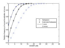
Figure 1: Probability of correct localization of errors using the subspace and extended subspace approaches, at different channel-error-to-quantization-noise ratio (CEQNR), for a $(10,5)$ DFT code where all errors are in even positions.

Remark 1.

Similar to the subspace approach [10], the extended subspace approach can be applied to the DCT and DST codes; further, it can be used even for the non-BCH DCT and DST codes [10].

Remark 2.

Knowing that $\tilde{R}_{m}$ can also be used to determine the number of errors $\nu$ [9], where the extended error localization is applicable, $\tilde{R}^{\prime}_{m}$ can be used for this purpose and it improves the results reasonably.

IV Rate-Adaptive Distributed Lossy Source Coding Using DFT Codes

Distributed lossless compression of two correlated sources can be as efficient as their joint compression [15]. This is also valid for lossy source coding with side information at the decoder for jointly Gaussian sources and the mean-squared error (MSE) distortion measure [16]. Tipically, DSC is realized by quantizing the sources and applying Slepian-Wolf coding in the binary domain. Slepian-Wolf coding can be implemented in the analog domain as well [4] which outperforms its binary counterpart for certain scenarios, e.g., an impulsive correlation model. The proposed DSC schemes based on DFT codes, both parity and syndrome approaches, are also appropriate for low-delay coding as they perform sufficiently well even when short source blocks are encoded.

When the statistical dependency between the sources varies or is not known at the encoder, a rate-adaptive system with feedback is an appealing solution [17]. Rate-adaptive DSC based on binary codes, e.g., puncturing the parity or syndrome bits of turbo and LDPC codes, have been proposed in [17, 18]. In the sequel, we extend DSC based on DFT codes [4] to perform DSC in a rate-adaptive fashion. We consider two continuous-valued correlated sources $\bm{x}$ and $\bm{y}$ where $x_{i}$ and $y_{i}$ are statistically dependent by $y_{i}=x_{i}+e_{i}$, and $e_{i}$ is continuous, i.i.d., and independent of $x_{i}$.

IV-A Parity-Based Approach

Puncturing is a well-known technique used to achieve higher rate codes for the same decoder; it is inherently well-suited for parity-based DSC schemes as one can remove some of the parity samples to puncture a code. However, with subspace error localizations, the performance of punctured DFT codes deteriorates largely. As explained in the previous section, extended subspace decoding significantly improves the results provided that the errors are restricted to even (odd) positions. This can be achieved by using $(2k,k)$ DFT codes. Generated by (1), a $(2k,k)$ DFT code is systematic with parity samples in even positions. We can modify this code and form a code whose parity samples are in the even positions [13]. Then, the extended syndrome matrix in (30) can be used both for error detection and localization. Similar to the subspace method, the performance of the system drops sharply with puncturing. Furthermore, although simple, puncturing may cause the minimum distance to decrease. An alternative, general approach for rate-adaptation is presented next.

IV-B Syndrome-Based Approach

Rate-adaption using puncturing is not natural for syndrome-based DSC systems [18]. Instead, the encoder can transmit a short syndrome based on an aggressive code and augment it with additional syndrome samples, if decoding fails. This process loops until the decoder gets sufficient syndrome for successful decoding. This approach is viable only for feedback channels with reasonably short round-trip time [17].

In the syndrome-based DSC based on DFT codes [4], the encoder computes $\bm{s}_{x}$ and transmits it to the decoder. At the decoder, we have access to the side information $\bm{y}=\bm{x}+\bm{e}$ and can compute its syndrome so as to find $\bm{s}_{e}=\bm{s}_{y}-\bm{{s}_{x}}$. For rate adaptation, if needed, the encoder transmits $\bar{\bm{s}}_{x}=\bar{H}\bm{x}$ sample by sample; the receiver also can compute $\bar{\bm{s}}_{y}=\bar{H}\bm{y}=\bar{\bm{s}}_{x}+\bar{\bm{s}}_{e}$ and evaluate $\bar{\bm{s}}_{e}=\bar{\bm{s}}_{y}-\bar{\bm{s}}_{x}$. After that, we can form the extended syndrome matrix $S^{\prime}_{m}$ by replacing $\bm{s}=\bm{s}_{e}$ and $\bar{\bm{s}}=\bar{\bm{s}}_{e}$ in the right-hand side of (35). Clearly, when quantization is considered this equation needs to be updated as

$$\tilde{s}^{\prime}_{m}=\left\{\begin{array}[]{l l}\tilde{s}_{m},&\quad 1\leq m\leq d,\\ \tilde{\bar{s}}_{m-d},&\quad d<m\leq n,\end{array}\right.$$ (38)

in which $\tilde{\bm{s}}=\bm{s}_{e}+\bm{s}_{q}$, $\tilde{\bar{\bm{s}}}=\bar{\bm{s}}_{e}+\bar{\bm{s}}_{q}$, and $\bar{\bm{s}}_{q}=\bar{H}\bm{q}$.

The new $\tilde{R}^{\prime}_{m}=\tilde{S}^{\prime}_{m}\tilde{S}^{\prime H}_{m}$ then is used for error localization as detailed in Section III. Note that the code is incremental, so the encoder does not need to re-encode the sources when more syndrome is requested. It buffers and transmits syndrome to the decoder sample by sample. Moreover, we can use $\tilde{R}^{\prime}_{m}$ to find the number of errors as explained in [9].

V Simulation Results

To evaluate the performance of the algorithm we do simulation using a Gauss-Markov source with mean zero, variance one, and correlation coefficient 0.9 for two DFT codes, namely, $(10,5)$ and $(17,9)$. For each code, we generate the syndrome and extended syndrome, quantize them with a 3-bit uniform quantizer with step size $\Delta=0.25$, and transmit them over a noiseless communication media. We plot the relative frequency of correct localization of different numbers of errors. To do so, we define channel-error-to-quantization-noise ratio (CEQNR) as the ratio of channel error power to the quantization noise power ($\sigma_{e}^{2}/\sigma_{q}^{2}$) and, similar to [8], we assume that the channel error components are fixed. The number of errors in each block is limited to $t$, the error correction capacity of the code. The simulation results are for $10^{4}$ input blocks for each CEQNR.

In Fig. 2, we compare the frequency of correct localization of errors for the subspace and extended subspace approaches given a $(10,5)$ code for different errors. The gain due to the extended subspace method is remarkable both for one and two errors; it is more significant for two errors. In fact, as discussed in Section III-A, for $\nu=t$ the subspace approach loses its degrees of freedom (DoF) and its performance drops to that of the coding-theoretic approach. Providing some extra DoF, at the expense of a higher code rate, the extended subspace approach significantly improves the error localization. Figure 3 shows how error localization boosts up when the additional syndrome samples are involved one by one. This allows doing DSC using DFT codes in a rate-adaptive manner.

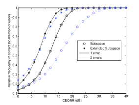
Figure 2: Probability of error localization in the subspace and extended subspace methods at different CEQNRs for a $(10,5)$ DFT code. The curves for the extended case are based on 3 additional syndrome samples, implying that the code rate is increased from 0.5 to 0.8.

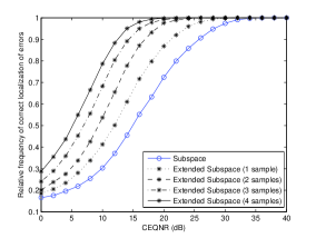
Figure 3: Probability of correct localization of 2 errors for a $(10,5)$ DFT code using the subspace method and the extended subspace method with different number of additional syndrome samples. The the code rate is increased from 0.5 to 0.9 by a step of 0.1.

The gain caused by the extended subspace method increases for codes with higher capacity. For instance, simulation results for a $(17,9)$ DFT code, presented in Fig. 4, show a significant gain in any CEQNR between $10$ to $40$dB; this is achieved by sending 4 additional syndrome samples.

It is also worth mentioning that numerical results proves the superiority of using $\tilde{R}^{\prime}_{m}$, instead of $\tilde{R}_{m}$ for finding the number of errors. Finally, since a better error localization implies a lower reconstruction error [9], rate-adapted DFT codes with extended subspace decoding can be used both to adapt the channel variations and decrease the MSE in DSC.

VI Conclusion

We developed two algorithms for rate-adaptation in the DSC system that uses DFT codes for binning. Rate-adaptation is realized by puncturing the parity samples in the parity-based DSC, or augmenting the syndrome samples in the syndrome-based DSC. For decoding, we introduced an extension of subspace error localization algorithm that substantially improves the error detection and localization, for a slight increase in the code rate. Interestingly, the gain caused by the extended subspace approach increases when capacity of the code or the number of errors go up. While the algorithm was successfully applied to the syndrome-based DSC in general, we have been able to exploit it only for the codes with rate $0.5$ in the parity-based system. The extended decoding algorithm can be applied to DCT and DST codes, as well.

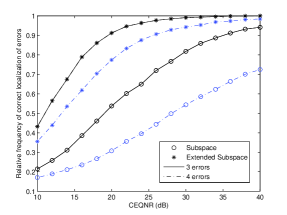
Figure 4: Probability of error localization in the subspace and extended subspace methods at different CEQNRs for a $(17,9)$ DFT code. The curves for the extended case are based on 4 additional syndrome samples.

References

- [1] R. E. Blahut, Algebraic Codes for Data Transmission. New York: Cambridge Univ. Press, 2003.
- [2] Z. Wang and G. B. Giannakis, “Complex-field coding for OFDM over fading wireless channels,” IEEE Trans. Inf. Theory, vol. 49, pp. 707–720, March 2003.
- [3] A. Gabay, M. Kieffer, and P. Duhamel, “Joint source-channel coding using real BCH codes for robust image transmission,” IEEE Trans. Image Process., vol. 16, pp. 1568–1583, June 2007.
- [4] M. Vaezi and F. Labeau, “Distributed lossy source coding using real-number codes,” in Proc. IEEE VTC Fall, pp. 1–5, 2012.
- [5] V. K. Goyal, J. Kovačević, and J. A. Kelner, “Quantized frame expansions with erasures,” Appl. Comput. Harmon. Anal., vol. 10, no. 3, pp. 203–233, 2001.
- [6] G. Rath and C. Guillemot, “Frame-theoretic analysis of DFT codes with erasures,” IEEE Trans. on Signal Process., vol. 52, pp. 447–460, Feb. 2004.
- [7] B. G. Bodmann and P. K. Singh, “Burst erasures and the mean-square error for cyclic Parseval frames,” IEEE Trans. Inf. Theory, vol. 57, pp. 4622–4635, July 2011.
- [8] G. Rath and C. Guillemot, “Subspace algorithms for error localization with quantized DFT codes,” IEEE Trans. Commun., vol. 52, pp. 2115–2124, Dec. 2004.
- [9] M. Vaezi and F. Labeau, “Wyner-Ziv Coding in the Real Field Based on BCH-DFT Codes,” [Online]. Available: http://arxiv.org/abs/1301.0297.
- [10] A. Kumar and A. Makur, “Improved coding-theoretic and subspace-based decoding algorithms for a wider class of DCT and DST codes,” IEEE Trans. Signal Process., vol. 58, pp. 695–708, Feb. 2010.
- [11] T. Marshall Jr., “Coding of real-number sequences for error correction: A digital signal processing problem,” IEEE J. Sel. Areas Commun., vol. 2, pp. 381–392, Mar. 1984.
- [12] R. E. Blahut, Algebraic Methods for Signal Process. and Commun. Coding. New York: Springer-Verlag, 1992.
- [13] M. Vaezi and F. Labeau, “Systematic DFT frames: Principle and eigenvalues structure,” in Proc. ISIT, pp. 2436–2440, 2012.
- [14] S. Kay, Modern Spectral Estimation. Englewood Cliffs, N.J.: Prentice-Hall, 1988.
- [15] D. Slepian and J. K. Wolf, “Noiseless coding of correlated information sources,” IEEE Trans. Inf. Theory, vol. IT-19, pp. 471–480, July 1973.
- [16] A. D. Wyner and J. Ziv, “The rate-distortion function for source coding with side information at the decoder,” IEEE Trans. Inf. Theory, vol. 22, pp. 1–10, Jan. 1976.
- [17] D. Varodayan, A. Aaron, and B. Girod, “Rate-adaptive codes for distributed source coding,” Signal Process., vol. 86, pp. 3123–3130, Nov. 2006.
- [18] V. Toto-Zarasoa, A. Roumy, and C. Guillemot, “Rate-adaptive codes for the entire Slepian-Wolf region and arbitrarily correlated sources,” in Proc. ICASSP, pp. 2965–2968, 2008.