Quantum information and statistical mechanics: an introduction to frontier

Abstract.

This is a short review on an interdisciplinary field of quantum information science and statistical mechanics. We first give a pedagogical introduction to the stabilizer formalism, which is an efficient way to describe an important class of quantum states, the so-called stabilizer states, and quantum operations on them. Furthermore, graph states, which are a class of stabilizer states associated with graphs, and their applications for measurement-based quantum computation are also mentioned. Based on the stabilizer formalism, we review two interdisciplinary topics. One is the relation between quantum error correction codes and spin glass models, which allows us to analyze the performances of quantum error correction codes by using the knowledge about phases in statistical models. The other is the relation between the stabilizer formalism and partition functions of classical spin models, which provides new quantum and classical algorithms to evaluate partition functions of classical spin models.

1. Introduction

Quantum information science is a rapidly growing field of physics, which explores comprehensive understanding of extremely complex quantum systems. An ultimate goal is building quantum computer or quantum simulator, which outperform conventional high performance (classical) computing. To achieve this goal, there still exist a lot of problems to be overcome. One of the main obstacles is decoherence, i.e., loss of coherence, due to an undesirable interaction between environments. Without a fault-tolerant design, any promising computing scheme is nothing but pie in the sky. Actually it has been shown that NP-complete problems (even PSPACE-complete problems), which are though to be intractable in classical digital computer, can be solved in polynomial time by using analog computer that can perform $x+y$, $x-y$, $xy$, and $\lfloor x\rfloor$ for any two real numbers $x$ and $y$ [1, 2]. However, such an analog computer has not been realized so far, since unlimited-precision real numbers cannot be physically realizable. Fortunately, in quantum computation, we have a fault-tolerant theory [3, 4, 5, 6, 7, 8, 9, 10], which guarantees an arbitrary accuracy of quantum computation as long as noise levels of elementary quantum gates are sufficiently smaller than a constant value, the so-called threshold value. Fault-tolerant quantum computation utilizes quantum error correction [3] to overcome decoherence, where we utilize many physical particles and classical processing to infer the error location. Another important problem for quantum computation is to identify the class of problems that can be solved by using quantum computer. Of course, we already have several quantum algorithms, Shor’s factorization [11], Grover’s search [12], etc., which outperform existing classical algorithms. However, these instances are not enough to understand the whole class of problems that quantum computer can solve, i.e., BQP problems, since they are, so far, not shown to be BQP-complete. Finding a good BQP-complete problem will lead us to a deeper understanding.

Interestingly, in both fault-tolerant quantum computing and finding new quantum algorithms, the idea of statistical mechanics has been applied, recently. One is a correspondence between quantum error correction and spin glass theory [13], where posterior probabilities in Bayesian inference problems for quantum error correction are mapped onto partition functions of spin glass theory. Thus the knowledge about phases in spin glass theory tells us the performance of quantum error correction codes [14, 15, 16, 17, 18, 19, 20, 21, 22]. Another is a relationship between overlaps (inner products) of quantum states and partition functions of statistical mechanical models [23, 24, 25]. Since the overlaps (inner products) can be estimated efficiently in quantum computer, this mapping gives us a new quantum algorithm to calculate the partition functions. Are these correspondences between quantum information and statistical mechanics accidental or inevitable? At least there is one common idea behind them, stabilizer states or stabilizer formalism [26], which might be an important clew to bridge the two fields and find new things.

The stabilizer states are a class of quantum states, which takes quite important roles in quantum information processing. The stabilizer formalism provides an efficient tool to provide a class of quantum operations on stabilizer states. In this review, we give a pedagogical introduction to the stabilizer formalism. Then we review two interesting interdisciplinary topics between quantum information science and statistical mechanics: the correspondence between quantum error correction and spin glass theory and the relation between the stabilizer formalism and partition functions of statistical models.

The rest of the paper is organized as follows: In Sec. 2, we introduce quantum-bit and elementary gates (unitary matrices). In Sec. 3, we introduce the stabilizer formalism. In Sec. 4, we explain how to describe a class of unitary operations and measurements on the stabilizer states in the stabilizer formalism. In Sec. 5, we demonstrate utility of the stabilizer formalism on the graph states [27], which are also an important class of quantum states associated with mathematical graphs. Specifically, we explain how Pauli basis measurements transform the graph states. Furthermore, we also introduce a model of quantum computation, measurement-based quantum computation. In Sec. 6, we review the relation between quantum error correction codes and spin glass models. In the last part of Sec. 6, we also mention a route toward building a fault-tolerant quantum computer. In Sec. 7, we review the relation between the stabilizer formalism and partition functions of classical spin models. As an exercise, we also show a duality relation between two distinct spin models by using the stabilizer formalism. Section 8 is devoted to a conclusion.

2. Quantum bit and quantum gates

In classical information science, the minimum unit of information is described by a binary digit or bit, which takes a value either 0 or 1. Its quantum counterpart is a quantum bit, so-called qubit. Qubit is defined as a superposition of two orthogonal quantum states $|0\rangle$ and $|1\rangle$, $|\psi\rangle=\alpha|0\rangle+\beta|1\rangle$, where $\alpha$ and $\beta$ are arbitrary complex values satisfying $|\alpha|^{2}+|\beta|^{2}=1$. An $n$-qubit state is described by

$$|\Psi\rangle=\sum_{i_{1},i_{2},...,i_{n}}C_{i_{1}i_{2}...i_{n}}|i_{1}i_{2}...i_{n}\rangle,$$

where $|i_{1}i_{2}...i_{n}\rangle\equiv|i_{1}\rangle\otimes|i_{2}\rangle\otimes...\otimes|i_{n}\rangle$. Since time evolutions are given by unitary operators in quantum physics, gate operations for a single qubit can be given by $2\times 2$ unitary matrices. The most fundamental gates are identity and Pauli operators:

$$I=\left(\begin{array}[]{cc}1&0\\ 0&1\end{array}\right),X=\left(\begin{array}[]{cc}0&1\\ 1&0\end{array}\right),Y=\left(\begin{array}[]{cc}0&-i\\ i&0\end{array}\right),Z=\left(\begin{array}[]{cc}1&0\\ 0&-1\end{array}\right).$$

The set of tensor products of the Pauli matrices on the $n$-qubit system $\{\pm 1,\pm i\}\times\{I,X,Y,Z\}^{\otimes n}$ forms the $n$-qubit Pauli group $\mathcal{P}_{n}$. A Pauli operator $A\in\{X,Y,Z\}$ acting on the $i$th qubit is denoted by $A_{i}\equiv I_{1}\otimes...\otimes I_{i-1}\otimes A_{i}\otimes I_{i+1}\otimes...\otimes I_{n}$.

In stead of the computational basis $\{|0\rangle,|1\rangle\}$, we may also choose different orthogonal bases:

$$\{|+\rangle\equiv(|0\rangle+|1\rangle)/\sqrt{2},|-\rangle\equiv(|0\rangle-|1\rangle)/\sqrt{2}\},\textrm{ or }\{|+i\rangle\equiv(|0\rangle+i|1\rangle)/\sqrt{2},|-i\rangle\equiv(|0\rangle-i|1\rangle)/\sqrt{2}\}.$$

The Hadamard and phase gates are defined as

$$H=\frac{1}{\sqrt{2}}\left(\begin{array}[]{cc}1&1\\ 1&-1\end{array}\right)\textrm{ and }S=\left(\begin{array}[]{cc}1&0\\ 0&i\end{array}\right).$$

These gates transform the computational bases, $\{|0\rangle,|1\rangle\}\leftrightarrow\{|+\rangle,|-\rangle\}$ and $\{|+\rangle,|-\rangle\}\leftrightarrow\{|+i\rangle,|-i\rangle\}$, respectively. These $X$, $Y$, $Z$, $H$ and $S$ gates are normalizers of the Pauli group and generate a group $\mathcal{C}_{1}$of single-qubit Clifford gates. (That is, a Clifford gate, say $A\in\mathcal{C}_{1}$, transforms the single-qubit Pauli group onto itself under the conjugation $A[\cdot]A^{{\dagger}}$. For example, $HXH=Z$, $SXS^{{\dagger}}=Y$, and so on.) Since the single-qubit Clifford group is a discrete group, one cannot generate arbitrary single-qubit unitary operations. Fortunately, it has been known that the existence of a non-Clifford gate in addition to the Clifford gates is enough for an efficient construction of an arbitrary single-qubit gate with arbitrarily high accuracy according to the Kitaev-Solovay theorem [28]. A non-Clifford gate can be, for example, $\pi/8$ gate $U_{\pi/8}=e^{-i\pi Z/8}$.

Single-qubit gates are not enough for constructing an arbitrary $n$-qubit unitary matrix, and hence at least one two-qubit gate operation is inevitable. There are two famous two-qubit gates, controlled-NOT (CNOT) and controlled-$Z$ (C$Z$) gates, which are given, respectively, by

$$\Lambda(X)_{c,t}=|0\rangle\langle 0|_{c}\otimes I_{t}+|1\rangle\langle 1|_{c}\otimes X_{t},\;\;\;\;\Lambda(Z)_{c,t}=|0\rangle\langle 0|_{c}\otimes I_{t}+|1\rangle\langle 1|_{c}\otimes Z_{t}.$$

Here a controlled-$A$ gate is denoted by $\Lambda(A)_{c,t}$, where the gate $A$ acts on the state labeled by $t$ conditioned on the state labeled by $c$. Thus these qubits $c$ and $t$ are called control and target qubits, respectively. These two two-qubit gates are both Clifford gates, that is, $\Lambda(A)$ ($A=X,Z$) transforms $\mathcal{P}_{2}$ onto itself under the conjugation $\Lambda(A)[\cdots]\Lambda(A)^{{\dagger}}$. For example, $\Lambda(X)_{c,t}X_{c}\otimes I_{t}\Lambda(X)_{c,t}^{{\dagger}}=X_{c}\otimes X_{t}$, $\Lambda(X)_{c,t}I_{c}\otimes Z_{t}\Lambda(X)_{c,t}^{{\dagger}}=Z_{c}\otimes Z_{t}$, $\Lambda(Z)_{c,t}X_{c}\otimes I_{t}\Lambda(Z)_{c,t}^{{\dagger}}=X_{c}\otimes Z_{t}$, and so on. It is known that an arbitrary unitary operation of $n$ qubits can be constructed from these elementary gates $\{H,S,U_{\pi/8},\Lambda(X)\}$ or $\{H,S,U_{\pi/8},\Lambda(Z)\}$. Such a set of elementary unitary gates is called a universal set, which is an instruction set of quantum computer.

3. Stabilizer states

In general, a description of quantum states is difficult since it requires exponentially many parameters in the number of qubits as shown in Eq. (2). To understand such a complex quantum system, efficient tools to describe important classes of complex quantum systems are essential. The matrix-product-states (MPS) [29], projected-entangled-pair-states (PEPS) [30, 31, 32], and multiscale-entanglement-renormalization-ansatz (MERA) [33] are such examples. The stabilizer states are another important class of quantum states, which take important roles in quantum information processing.

Now we introduce the definition of stabilizer states and the stabilizer formalism [26]. We define a stabilizer group $\mathcal{S}$ of an $n$-qubit system as an Abelian subgroup of the $n$-qubit Pauli group that does not includes $-I$ as its element. In other words, all elements in the stabilizer group are commutable with each other and hermitian. For example, a set

$$\mathcal{S}_{\rm Bell}=\{II,XX,ZZ,-YY\}$$

is a two-qubit stabilizer group, where $A\otimes B$ is denoted by $AB$ for simplicity.

The stabilizer group $\mathcal{S}$ can be defined in terms of the maximum independent set of the stabilizer group, which we call stabilizer generators. Here independence is defined such that each element in the generator set cannot be expressed as a product of other elements in the generator set. The stabilizer group generated by a stabilizer generators $\{S_{i}\}$ is denoted by $\langle\{S_{i}\}\rangle$. For example, the stabilizer group $\mathcal{S}_{\rm Bell}=\{II,XX,ZZ,-YY\}$ can be written simply by $\langle XX,ZZ\rangle$. Any stabilizer group of $n$ qubits can be defined if at most $n$ stabilizer generators are given.

The stabilizer state is defined as a simultaneous eigenstate of all stabilizer elements with the eigenvalue +1. It is sufficient that the state is an eigenstate of all stabilizer generators:

$$S_{i}|\psi\rangle=|\psi\rangle\textrm{ for all stabilizer generators }S_{i}.$$

The dimension $2^{d}$ of the space spanned by the stabilizer states is calculated to be $2^{d}=2^{n-k}$ with $n$ and $k$ being the number of qubits and stabilizer generators, respectively. This can be understood that the $2^{n}$-dimensional space is divided into two orthogonal subspaces for each stabilizer generator.

For example, the stabilizer state defined by the stabilizer group $\mathcal{S}_{\rm Bell}=\langle XX,ZZ\rangle$ is $(|00\rangle+|11\rangle)/\sqrt{2}$, which is a maximally entangled state of two qubits [34]. The maximally entangled state is a useful resource for teleporting an unknown quantum state between two separate sites, that is, quantum teleportation [35].

Another representative example of the stabilizer states is an $n$-qubit cat state,

$$|{\rm cat}\rangle=\frac{1}{\sqrt{n}}(|00...0\rangle+|11...1\rangle),$$

whose stabilizer group is given by

$$\left\langle Z_{1}Z_{2},\;...,\;Z_{n-1}Z_{n},\;\prod_{i=1}^{n}X_{i}\right\rangle,$$

where $A_{i}$ indicates a Pauli operator $A\in\{X,Y,Z\}$ on the $i$th qubit. The cat state is a representative example of macroscopically entangled states. If one particle is determined whether it is $|0\rangle$ or $|1\rangle$, the superposition is completely destroyed.

4. Quantum operations on stabilizer states

Let us consider the action of a Clifford gate $U$ on the stabilizer state $|\psi\rangle$ defined by a stabilizer group $\mathcal{S}=\langle\{S_{i}\}\rangle$:

$$U|\psi\rangle=US_{i}|\psi\rangle=US_{i}U^{{\dagger}}U|\psi\rangle=S^{\prime}_{i}U|\psi\rangle,$$

where $S^{\prime}_{i}\equiv US_{i}U^{{\dagger}}$. This indicates that a state $U|\psi\rangle$ is an eigenstate of the operator $S^{\prime}_{i}$ with an eigenvalue +1 for all $S^{\prime}_{i}$. Furthermore, since the Clifford group of unitary gates are normalizer of the Pauli group (and hence a Pauli product is transformed to another Pauli product under its conjugation), the group $\mathcal{S}^{\prime}=\langle\{S^{\prime}_{i}\}\rangle$ is also a stabilizer group. That is, $U|\psi\rangle$ is the stabilizer state defined by the stabilizer group $\mathcal{S}^{\prime}$. In this way, the action of $U$ on the stabilizer state can be regarded by a map between the stabilizer groups. For example, a stabilizer group $\langle X_{1}I_{2},I_{1}Z_{2}\rangle$ (the corresponding state is $|+\rangle_{1}|0\rangle_{2}$) is transformed to $\langle X_{1}X_{2},Z_{1}Z_{2}\rangle$ (the corresponding state is $(|00\rangle+|11\rangle)/\sqrt{2}$) by $\Lambda(X)_{1,2}$.

The projective measurement of a hermitian Pauli product as an observable can also be described by a map between stabilizer groups as follows. Suppose $A$ is an $n$-qubit hermitian Pauli product and $P_{\pm}=(I\pm A)/2$ are the corresponding projection operators. Due to the projective measurement, a state $|\psi\rangle$ is projected to $P_{+}|\psi\rangle/\sqrt{||P_{+}|\psi\rangle||}$ or $P_{-}|\psi\rangle/\sqrt{||P_{-}|\psi\rangle||}$ with probabilities $||P_{\pm}|\psi\rangle||$. For simplicity, we consider the case with the measurement outcome $+$. There are three possibilities:

• $A$ (or $-A$) is an element of the stabilizer group.

• While $A$ (or $-A$) does not belong to the stabilizer group, $A$ is commutable with all elements of the stabilizer group.

• At least one stabilizer operator does not commute with $A$.

In the case (i), the state does not change. In the case (ii), the stabilizer group for the post-measurement state is given by $\langle A,\{S_{i}\}\rangle$. That is, $A$ is added to the generator set. In the case (iii), we can always choose a generator set $\langle S_{1},S_{2},...S_{k}\rangle$ ($k<n$) of the original stabilizer group such that $A$ commutes with all generators $S_{2},...,S_{k}$ except for $S_{1}$. Then the stabilizer group of the post-measurement state is given by $\langle A,S_{2},...,S_{k}\rangle$. That is, in addition to adding $A$, $S_{1}$ is removed from the generator set.

5. Graph states

In this section, we exercise to use the stabilizer formalism. As an example of the stabilizer states, we use the most important subclass of stabilizer states, graph states [27]. A graph state is defined associated with a graph $G(V,E)$, where $V$ and $E$ are the sets of the vertices and edges, respectively. A qubit is located on each vertex of the graph. The stabilizer generator of the graph state $|\psi_{G}\rangle$ associated with a graph $G(V,E)$ is given by

$$K_{i}=X_{i}\prod_{j\in N_{i}}Z_{j}\;\;\textrm{for all }i\in V,$$

where the neighbor $N_{i}:=\{j|(i,j)\in E\}$ of vertex $i$ indicates the set of vertices that are connected to vertex $i$ on the graph.

Each stabilizer generator $K_{i}$ is transformed to $X_{i}=UK_{i}U$ by $U=\prod_{(i,j)\in E}\Lambda(Z)_{i,j}$, where we aggressively used the fact that $\Lambda(Z)_{i,j}X_{i}I_{j}\Lambda(Z)_{i,j}=X_{i}Z_{j}$. This fact indicates that $U$ transforms the stabilizer group from $\langle\{K_{i}\}_{i\in V}\rangle$ to $\langle\{X_{i}\}_{i\in V}\rangle$. The stabilizer state defined by the latter is $|+\rangle^{\otimes|V|}$ where $|V|$ is the number of the vertices. This implies that we can obtain the graph state $|\psi_{G}\rangle$ from the product state $|+\rangle^{\otimes|V|}$ as $|\psi_{G}\rangle=U|+\rangle^{\otimes|V|}$. Specifically, when the graphs are regular such as one-dimensional, square, hexagonal, and cubic lattices, the corresponding graph states are also referred to as cluster states [36]. It has been known that any stabilizer state is equivalent to a certain graph state up to local Clifford operations [37, 27]. However, the graph associated with a stabilizer state is not uniquely defined, since there exist local Clifford operations that change the associated graph. This property is called local complementarity of the graph states [37, 27].

Next we will see how Pauli basis measurements transform the graph states. Let us consider a one-dimensional graph state as shown in Figs. 1 (a)-(c). At first, we consider the $Z$ basis measurement (projective measurement of the observable $Z$) on the $i$th qubit. The stabilizer group for the post-measurement state is given by

$$\langle...,K_{i-1},Z_{i},K_{i+1},...\rangle,$$

since $K_{i}$ does not commute with $Z_{i}$. After the projection, the $i$th qubit is $|0\rangle$ and hence decoupled with the other qubits. By rewriting the stabilizer generators, we obtain three decoupled stabilizer groups

$$\langle...,Z_{i-2}X_{i-1}\rangle,\langle Z_{i}\rangle,\langle X_{i+1}Z_{i+2},...\rangle,$$

which means the graph is separated by the $Z$ basis measurement as shown in Fig. 1 (a).

Similarly, we consider the $X$-basis measurement. Since $X_{i}$ does not commute with $K_{i-1}$ and $K_{i+1}$ but commutes with $K_{i-1}K_{i+1}=Z_{i-2}X_{i-1}X_{i+1}Z_{i+2}$, the stabilizer group for the post-measurement state is given by

$$\langle...,Z_{i-2}X_{i-1}X_{i+1}Z_{i+2},Z_{i-1}Z_{i+1},...\rangle,\langle X_{i}\rangle.$$

By performing the Hadamard gate $H$ on the $(i-1)$th qubit, we obtain a new stabilizer group

$$\langle...,Z_{i-2}Z_{i-1}X_{i+1}Z_{i+2},X_{i-1}Z_{i+1},...\rangle,\langle X_{i}\rangle,$$

which indicates that the graph is transformed as shown in Fig. 1 (b) up to the Hadamard gate. Instead of the $(i-1)$th qubit, we can obtain a similar result by performing the Hadamard gate on the $(i+1)$th qubit.

The final example is the $Y$-basis measurement. Since $Y_{i}$ does not commute with $K_{i-1}$, $K_{i}$ and $K_{i+1}$ but commutes with $K_{i-1}K_{i}=Z_{i-2}Y_{i-1}Y_{i}Z_{i+1}$, and $K_{i}K_{i+1}=Z_{i-1}Y_{i}Y_{i+1}Z_{i+2}$, the stabilizer group for the post-measurement state is given by

$$\langle...,Z_{i-2}Y_{i-1}Z_{i+1},Z_{i-1}Y_{i+1}Z_{i+2},...\rangle,\langle Y_{i}\rangle.$$

By performing the phase gates $S$ on the $(i-1)$th and $(i+1)$th qubits, we obtain a new stabilizer group

$$\langle...,Z_{i-2}X_{i-1}Z_{i+1},Z_{i-1}X_{i+1}Z_{i+2},...\rangle,\langle Y_{i}\rangle.$$

This indicates that the graph is directly connected up to the phase gates as shown in Fig. 1 (c).

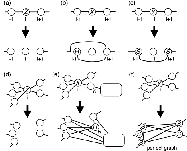
Figure 1. The transformations of graph states by the Pauli basis measurements. (a) The $Z$-basis measurement on a one-dimensional graph state. (b) The $X$-basis measurement on a one-dimensional graph state. $H$ indicates the Hadamard gate. (c) The $Y$-basis measurement on a one-dimensional graph state. $S$s indicates the phase gates. (d) The $Z$-basis measurement on a general graph state. The edges incident to the $i$th (measured) qubit is removed. (e) The $X$-basis measurement on a general graph state. A qubit $h$ is chosen from the set $V_{i}$ of qubits connected to the $i$th (measured) qubit. All edges connected to the $i$th qubit are removed, and the edges between $V_{i}\setminus h$ and $h$ and between $V_{i}\setminus h$ and vertices which are connected with $h$ (shown by a blank box) are added. In addition, the $H$ gate is performed on the $h$th qubit. For arbitrary choices of $h\in V_{i}$, the associated graph states, which are equivalent up to local Clifford gates with each other, are defined. (f) The $Y$-basis measurement on a general graph state. All edges connected to the $i$th qubit are removed. Instead, a complete graph of the vertices $V_{i}$ adjacent to the $i$th (measured) qubits is added. In addition, the $S$ gates are performed on the qubits belonging to $V_{i}$.

The actions of the Pauli basis measurements for general graph structures can be also calculated in a similar manner as shown in Fig. 1 (d)-(f), where no loop is included for clarity, but their extensions to arbitrary graphs are straightforward.

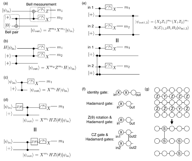
Figure 2. (a) A circuit for quantum teleportation [35]. The two-qubit gates are the CNOT gates, where the control and target qubits are denoted by black and white circles, respectively. (b) An equivalent circuit of (a), which consists of the C$Z$ gates. The Hadamard gates come from the equivalence $\Lambda(X)_{c,t}=H_{t}\Lambda(Z)_{c,t}H_{t}$. (c) A minimum unit of teleportation-based gate, which transforms the input state to the output with the Hadamard operation. (d) The circuit equivalence for the $HZ(\theta)$ operation. The measurement in the $X$ basis after the $Z(\theta)$ rotation teleports the output state with the $HZ(\theta)$ operation up to a Pauli byproduct. (e) The C$Z$ gate for the output states (upper circuit) can be moved into the generation of a graph state (lower circuit), where the commutability of C$Z$ gates is utilized. (f) Graph diagrams of MBQC. From top to bottom, they describe the identity gate (b), the Hadamard gate (c), the $Z(\theta)$ rotation followed by the Hadamard gate (d), and the teleportation-based C$Z$ gate followed by the Hadamard gates (e). (g) A graph state required for quantum computation is generated from the 2D cluster state on a square lattice by using Pauli basis measurements.

The graph states take important roles in quantum information processing [27]. First of all, graph states defined on a certain class of graphs, such as square and hexagonal lattices, can be used for resources for measurement-based quantum computation (MBQC) [38, 39, 40, 41]. This can be understand as follows. The circuit in Fig. 2 (a) is well-known quantum teleportation [35], where a Bell pair $(|00\rangle+|11\rangle)/\sqrt{2}$ is prepared as a resource, and the unknown input state is teleported into the output up to a Pauli byproduct depending on the measurement outcomes. This circuit is equivalent to that in Fig. 2 (b), which reads $X$-basis measurements on a graph state transfer the input state to the output state. Here we should recall that a graph state is generated by C$Z$ gates from $|+\rangle^{\otimes n}$. The measurement-based identity gate can be decomposed into two Hadamard gates, one of which is shown in Fig. 2 (c). By measuring in the $X$ basis after $Z(\theta)\equiv e^{-i\theta Z/2}$, a unitary transformation $HZ(\theta)$ can be performed in a teleportation-based way as shown in circuit equivalences in Fig. 2 (d). The Pauli byproduct made due to the probabilistic nature of measurements has to be always placed at the top of the output state to handle the nondeterminism. However, $Z(\theta)$ does not commute with the Pauli byproduct if it contains the Pauli $X$ operator, i.e., $Z(\theta)X=XZ(-\theta)$. To settle this, the measurement angle $\theta$ is adaptively changed to $-\theta$ beforehand according to the previous measurement outcomes, which is called feedforward in MBQC.

By using commutability of C$Z$ gates as shown in Fig. 2 (e), the C$Z$ gate performed for the output of teleportation can be moved into the offline graph state preparation. This trick is the so-called quantum gate teleportation [42]. In this way, an arbitrary single qubit rotation and the C$Z$ gate, which are sufficient for universal quantum computation, can be implemented by adaptive measurements on a specific type of graph state Starting from, for example, a two-dimensional (2D) cluster state on a square lattice, we can generate an arbitrary graph state required for universal quantum computation by using Pauli basis measurements mentioned before. Roughly speaking, the universality of measurement-based quantum computation means that by performing measurements in appropriately chosen bases $\{|\alpha_{i}\rangle\}$, the output of a quantum computation $U|0\rangle^{\otimes n}$ of $n$ qubits can be simulated as

$$U|0\rangle^{\otimes n}=2^{(|V|-n)/2}\left(\bigotimes_{i\in V\verb+\+\textrm{output $n$ qubits}}\langle\alpha_{i}|\right)|\psi_{G}\rangle.$$ (3)

Such a state, which allows universal quantum computation in a measurement-based way, is called universal resource. Recently, MBQC on more general many-body quantum states has been proposed [43, 44], which utilizes MPS and PEPS as resources. MBQC on ground or thermal states of valence-bond-solid systems have been proposed [45, 46, 47, 49, 48, 50, 51], which might be useful to relax experimental difficulties in preparations of universal resources for quantum computation.

6. Quantum error correction codes and spin glass models

In the following two sections, we will review the interdisciplinary topics between quantum information science and statistical mechanics. In this section, we describe the correspondence between quantum error correction codes and spin glass models.

Quantum error correction [3] is one of the most successful schemes to handle errors on quantum states originated from an undesirable interaction with environments. Quantum error correction codes employ multiple physical qubits to encode logical information into a subspace, so-called code space. The stabilizer formalism is vital to describe such a complex quantum system. Below we will describe one of the most important quantum error correction codes, the surface code [52, 13], which has a close relation to a spin glass model, the random-bond Ising model (RBIM).

The surface code on the square lattice consists of qubits located on edges $i\in E$ of the square lattice [52, 13] (note that the location of qubits is different from that of the graph states). Specifically, we consider a periodic boundary condition, that is, the surface code on a torus. The face and vertex stabilizer operators of the surface code are defined for each face $f\in F$ and vertex $v\in V$ as

$$A_{f}=\prod_{i\in E_{f}}Z_{i},\textrm{ and }\;\;B_{v}=\prod_{j\in E_{v}}X_{j},$$

respectively [see Fig. 3 (a)]. Here $E_{f}$ and $E_{v}$ ($E_{f,v}\subset E$) indicate the sets of four edges that are surrounding the face $f$ and are adjacent to the vertex $v$, respectively. The code state $|\Psi\rangle$ is defined as the simultaneous eigenstate of all stabilizer operators with the eigenvalue $+1$:

$$|\Psi\rangle=A_{f}|\Psi\rangle,\;\;|\Psi\rangle=B_{v}|\Psi\rangle\textrm{ for all}\;\;f,v.$$

As will be seen below, the eigenvalues of these stabilizer operators are used to diagnose syndromes of errors.

The logical information encoded in the code space is defined by those operators that are commutable with all elements in the stabilizer group but are independent from them. Such operators characterize the degrees of freedom in the degenerated code space and hence called logical operators. The products of $Z$s on any trivial cycle of the lattice are commutable with stabilizer operators. But they are also elements of the stabilizer group, since they are written by the product of all $A_{f}$s inside the trivial cycle as shown in Fig. 3 (b). This is also the case for the products of $X$s on any trivial cycle of the dual lattice. The products of $Z$s ($X$s) on nontrivial cycles wrapping around the torus on the primal (dual) lattice give the logical operators, which we denote by $L_{Z}$ ($L_{X}$). Since the genus of the torus is one, we can find two pairs of logical operators $(L_{X}^{(1)},L_{Z}^{(1)})$ and $(L_{X}^{(2)},L_{Z}^{(2)})$ on the torus as shown in Fig. 3 (c). Note that the actions of the logical operators on the code space depend only on the homology class of the logical operators. Since these logical operators are subject to the Pauli commutation relation $L_{X}^{(i)}L_{Z}^{(j)}=-\delta_{ij}L_{Z}^{(j)}L_{X}^{(i)}$ and $(L_{A}^{(i)})^{2}=I$, they represent two logical qubits encoded in the code space. In general, a surface code defined on a surface of a genus $g$ can encode $2g$ logical qubits.

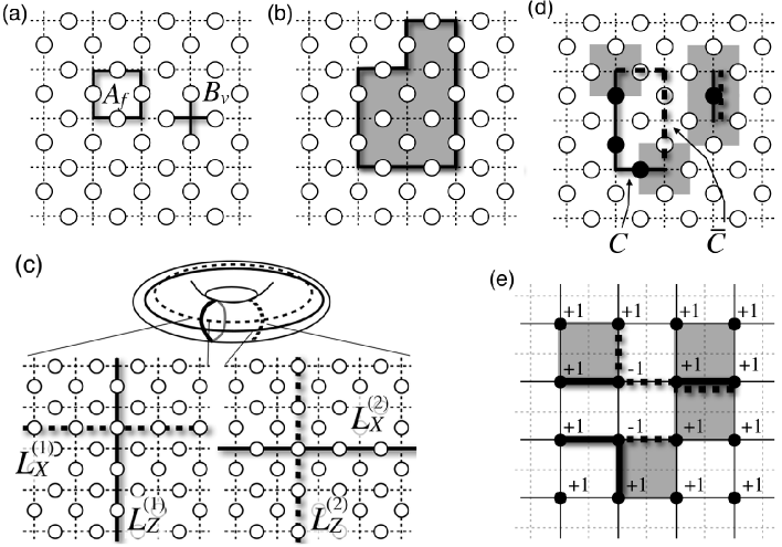
Figure 3. (a) The vertex and face stabilizer operators. (b) A trivial cycle. The product of the Pauli $Z$ operators on a trivial cycle is equivalent to the product of face stabilizer generators inside the cycle, and hence it belongs to the stabilizer group. (c) Two pairs of the logical operators, $L_{X}^{(1)}$ (left dotted line), $L_{Z}^{(1)}$ (left solid line), $L_{X}^{(2)}$ (right dotted line), and $L_{Z}^{(2)}$ (right solid line). (d) The black circles and solid lines denote a chain $C$ of $Z$ errors. The vertices with $b_{v}=-1$ are denoted by gray squares. The estimated chain $\bar{C}$ of errors for a recovery is shown by dotted lines. If $C+\bar{C}$ is a trivial cycle, the error correction succeeds. Otherwise if $C+\bar{C}$ is a nontrivial cycle, it changes the code space nontrivially. (e) RBIM on the dual lattice. The error chain $C$ corresponds to the locations of antiferromagnetic interactions. The recovery chain $\bar{C}$ corresponds to the excited domain wall. The vertices with $b_{v}=-1$ correspond to Ising vortexes. At zero temperature, a spin configuration is chosen so that the length of excited domain wall is minimum, i.e., MWPM of the Ising vortexes (or frustrations).

Let us consider how errors appear on the code state. We, for simplicity, consider the Pauli operators $X$ (bit-flip error) and $Z$ (phase-flip error) act on the code state with an identical and independent distribution. However, possibility of correcting these two types of errors guarantees the validity under a general noise model. While, in the following, we only consider how to correct $Z$ (phase-flip) errors for clarity, it is straightforward to correct $X$ (bit-flip) errors in the same manner. Suppose a chain of $Z$ errors occur on the set $C$ of the qubits (see Fig. 3 (d)). The code state is given by $|\Psi^{\prime}\rangle=\prod_{i\in E}Z_{i}^{u_{i}^{C}}|\Psi\rangle$, where $u^{C}_{i}=1$ if $i\in C$ and $u^{C}_{i}=0$ if $i\notin C$. Due to the errors, the state $|\Psi^{\prime}\rangle$ is not in the code space anymore. If $|E_{v}\cap C|$ is odd,

$$B_{v}|\Psi^{\prime}\rangle=-\left(\prod_{i\in E}Z_{i}^{u_{i}^{C}}\right)B_{v}|\Psi\rangle=-|\Psi^{\prime}\rangle$$

and hence the eigenvalue of the vertex stabilizer $B_{v}$ is flipped to $-1$. The error syndrome of a chain $C$ of $Z$ errors is defined as a set of eigenvalues $\{b_{v}=\pm 1\}$ of the vertex stabilizers $\{B_{v}\}$. Similarly the error syndrome of $X$ errors is defined as a set of eigenvalues $\{a_{f}=\pm 1\}$ of the face stabilizers $\{A_{f}\}$. The eigenvalues $b_{v}=-1$ are obtained at the boundaries $\partial C$ (grayed squares in Fig. 3 (d)) of the error chain $C$, since the vertex stabilizers anticommute with the error chain there. In order to recover from the errors, we infer the most likely error operator $\bar{C}_{\rm ML}$ which has the same error syndromes as $C$, i.e., $\partial\bar{C}_{\rm ML}=\partial C$. If $C+\bar{C}_{\rm ML}$ becomes a trivial cycle the error correction succeeds, since it acts on the code space trivially as a face stabilizer operator. Otherwise, if the chain $C+\bar{C}_{\rm ML}$ becomes a nontrivial cycle, the operator $\prod_{i\in E}Z_{i}^{C+\bar{C}_{\rm ML}}$ is a logical operator. Thus the recovery operation destroys the original logical information, meaning a failure of the error correction.

Suppose errors occur with an independent and identical probability $p$. (Note that $p$ is a parameter in the posterior probability of the inference problem, and hence can be different from the actual error probability $p^{\prime}$.) The error probability of an error chain $\bar{C}$ conditioned on the $\partial\bar{C}=\partial C$ becomes

$$P(\bar{C}|\partial\bar{C}=\partial C) = \mathcal{N}\prod_{i}\left(\frac{p}{1-p}\right)^{u^{\bar{C}}_{i}}\big{|}_{\partial\bar{C}=\partial C}=\mathcal{N}^{\prime}\exp\left[-\beta J\sum_{i}(2u^{\bar{C}}_{i}-1)\right]\big{|}_{\partial\bar{C}=\partial C}$$ (4)

where $\mathcal{N}$ and $\mathcal{N}^{\prime}$ are the normalization factors, $e^{-\beta J}\equiv\sqrt{p/(1-p)}$. The most likely error operator $\bar{C}_{\rm ML}$ conditioned on the syndrome $\partial C$ can be obtained by maximizing the posterior probability:

$$\bar{C}_{ML}={\rm arg}\;\max_{\bar{C}}\;P(\bar{C}|\partial\bar{C}=\partial C)={\rm arg}\;\min_{\bar{C}}\;\sum_{i}u^{\bar{C}}_{i}|_{\partial\bar{C}=\partial C}.$$

This indicates that the most likely chain $\bar{C}_{\rm ML}$ is an error chain that connects pairs of two boundaries with a minimum Manhattan length. Such a problem can be efficiently solved in classical computer by using the Edmonds’ minimum-weight-perfect-matching (MWPM) algorithm [53]. The accuracy threshold with the decoding by the MWPM algorithm has been estimated to be 10.3% (MWPM) [14].

The MWPM algorithm is not optimal for the present purpose, since we have to take not only the probability of each error $\bar{C}$ but also the combinatorial number of the error chains $\bar{C}$ such that $\bar{C}+C$ belongs to the same homology class (recall that the action of logical operators on the code state depends only on the homology class of the associated chains). By taking a summation over such a $\bar{C}$ that belongs to the same homology class, we obtain a success probability of the error correction

$$p_{\rm suc}=\mathcal{N}^{\prime\prime}\sum_{\bar{C}+C=\textrm{trivial cycles}}\exp\left[\beta J\sum_{i}v_{i}^{\bar{C}}\right],$$

where $v_{i}^{\bar{C}}=-2u_{i}^{\bar{C}}+1$ is defined. In order to simplify the summation over trivial cycles, we introduce an Ising spin $\sigma_{i}\in\{+1,-1\}$ on each face center (i.e., vertex of the dual lattice) of the lattice (see Fig. 3 (e)). If $\bar{C}+C$ a trivial cycle, there exists a configuration $\{\sigma_{i}\}$ such that $v_{l}^{\bar{C}}=v_{l}^{C}\sigma_{i}\sigma_{j}$ with $l$ being the bond between the spins $\sigma_{i}$ and $\sigma_{j}$. The variable $v_{l}$ located on the bond in-between the sites $i$ and $j$ is denoted by $v_{ij}$ hereafter. By using this fact, the success probability can be reformulated as

$$p_{\rm suc} = \mathcal{N}^{\prime\prime\prime}\sum_{\{\sigma_{i}\}}\exp\left[{\beta\sum_{\langle ij\rangle}J_{ij}\sigma_{i}\sigma_{j}}\right],$$

where $\mathcal{N}^{\prime\prime\prime}$ is a normalization factor, and $J_{ij}\equiv Jv_{ij}^{C}$.

Now that the relation between quantum error correction and a spin glass model becomes apparent; the success probability of the $Z$ error correction is nothing but the appropriately normalized partition function of the RBIM, whose Hamiltonian is given by $H=-\sum_{\langle ij\rangle}J_{ij}\sigma_{i}\sigma_{j}$. The location of $Z$ errors represented by $J_{ij}=-1$ corresponds to the anti-ferromagnetic interaction due to disorder, whose probability distribution is given by $P(J_{ij})=(1-p^{\prime})\delta(J_{ij}-1)+p^{\prime}\delta(J_{ij}+1)$. (Recall that the hypothetical error probability $p$ is given independently of the actual error probability $p^{\prime}$.) The error syndrome $b_{v}=-1$ corresponds to the frustration of Ising interactions (see Fig. 3 (e)). Equivalently it is also the end point (Ising vortex) of the excited domain wall.

In order to storage quantum information reliably, the success probability has to be reduced exponentially by increasing the system size. This is achieved with an error probability $p^{\prime}$ below a certain value, so-called accuracy threshold $p^{\rm th}$. However, if the error probability is higher than it, the success probability converges to a constant value. This drastic change on the function $p_{\rm suc}$ corresponds to a phase transition of the RBIM. Specifically, in the ferromagnetic phase, quantum error correction succeeds. (Actually the logical error probability is related to the domain-wall free-energy via $-(1/\beta)\ln p_{\rm suc}$. In the ferromagnetic phase, the domain-wall free-energy scales like $O(N)$ with $N$ being the vertical or horizontal dimension of the system. This supports the exponential suppression of logical errors.) Of course, we should take $p=1/(e^{2\beta}+1)=p^{\prime}$, that is, the actual and hypothetical error probabilities are the same, in order to perform a better error correction. This condition corresponds to the Nishimori line [54] on the $(\beta,p)$ phase diagram. The precise value of the optimal threshold has been calculated to be 10.9% [15], which is fairly in good agreement with the numerical estimation [55]. The threshold value 10.3% with the MWPM algorithm corresponds to the critical point at zero temperature, since the solution of the MWPM algorithm is obtained in the $\beta\rightarrow\infty$ limit.

Recently the surface codes have been also studied on general lattices including random lattices [15, 16, 17, 18, 19]. Furthermore, the performance analyses in the presence of qubit-loss error have been also argued [20, 21, 22, 17], which corresponds to bond dilution in the RBIM.

The surface code is one example of topological stabilizer codes, whose stabilizer operators are local (i.e., finite-body Pauli products) and translation invariant. A complete classification of topological stabilizer codes is obtained in Ref. [56]. Another well-studied example of topological stabilizer codes is the color codes [57, 58], which are related to the random three-body Ising models. The performance of the color codes has been also discussed via the spin glass theory [59, 60].

An important issue in quantum error correction, where the knowledge of statistical mechanics seems to be quite useful, is finding a fast classical decoding algorithm. Recently several new efficient algorithms have been proposed [62, 63, 64]. They are based on a renormalization group algorithm [62], local search [63], and parallel tempering [64], each of which is well studied in statistical mechanics.

In fault-tolerant quantum computation, we have to take all sources of errors into account, such as imperfections in syndrome measurements. Thus, in fault-tolerant quantum computation the code performances under perfect syndrome measurements are of limited interest. For both surface and color codes, their performances have been investigated under imperfect syndrome measurements [13, 14, 61]. Interestingly, the inference problems of errors in them are mapped into three-dimensional random ${\mathbf{Z}}_{2}$ gauge theories. Recently, topologically protected measurement-based quantum on the symmetry breaking thermal state has been proposed [65]. This model is mapped into a correlated random-plaquette ${\mathbf{Z}}_{2}$ gauge model, whose critical point on the Nishimori line is shown to be equivalent to that of the three-dimensional Ising model.

More comprehensive studies of fault-tolerant quantum computation has been taken by considering errors in state initializations, measurements, and elementary gate operations used in both quantum error correction itself and universal quantum computation on the code space [66, 67, 68, 69]. Based on these analyses, physical implementations and quantum architecture designs have been argued recently [70, 71, 72, 73, 74, 75, 76, 77, 78], which clarify the experimental requirements for building fault-tolerant quantum computer. On the other side, extensive experimental resources have been paid to achieve these requirements, and very encouraging results have already obtained in some experiments, for example, in trapped ions [80, 79] and superconducting systems [81, 82]. Finding a high performance quantum error correction code, an efficient classical algorithm for decoding, and a detailed analysis of an architecture under a realistic situation will further help an experimental realization of large scale quantum computer.

7. Statistical models and stabilizer formalism

In this section, we describe a mapping between the stabilizer formalism and classical statistical models [24, 25], which allows us to analyze classical statistical models via quantum information and vice versa.

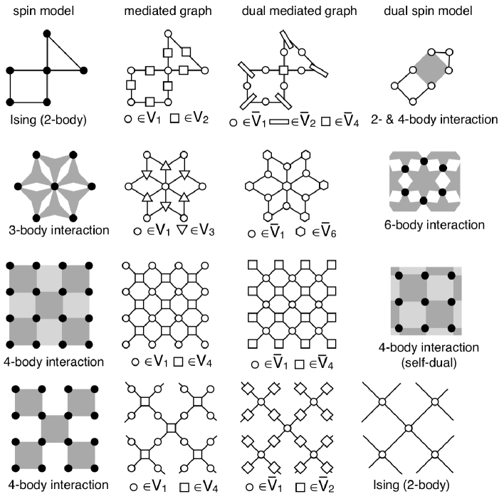
Figure 4. From left to right, spin models, corresponding mediated graph states, dual mediated graph states, and dual spin models. In the mediated graph states, circles indicate the qubits representing sites of spin models. The magnetic fields are given by a product state defined on these site qubits. The polygons indicate the qubits, which mediate the many-body interactions. The number of the edges of each polygon is equivalent to the number of spins engaged in the corresponding interaction. The coupling strengths of the many-body interactions are determined by a product state defined on these mediating qubits.

More precisely, we will relate an overlap $\langle\alpha|\Psi_{G}\rangle$ of a product state $|\alpha\rangle\equiv\prod_{i}|J_{i}\rangle$, which will be defined later in detail, and a graph state $|\Psi_{\rm G}\rangle$ to a partition function $\mathcal{Z}(\beta)$ of a spin model associated with interactions $J_{i}$:

$$\mathcal{Z}(\beta)=\frac{1}{2^{|V_{1}|/2}}\langle\alpha|\Psi_{G}\rangle,$$

where $|V_{1}|$ denotes the number of sites in the spin model. Since the right hand side can be efficiently evaluated by using quantum computer, the overlap mapping gives us an algorithm to calculate the partition functions. Below we explain a derivation of the overlap mapping in detail.

We consider a classical statistical model on a lattice $L$:

$$H=\sum_{i}J_{i}s_{i}+\sum_{\langle i,j\rangle}J_{i,j}(s_{i}\oplus s_{j})+\sum_{\langle i,j,k\rangle}J_{i,j,k}(s_{i}\oplus s_{j}\oplus s_{k})+\dots+\sum_{\langle i_{1},i_{2},...,i_{m}\rangle}J_{i_{1},i_{2},...,i_{m}}\left(\bigoplus_{j=1}^{m}s_{i_{j}}\right),$$

where $s_{i}\in\{0,1\}$ is the $i$th Ising spin variable, $J_{i_{1},i_{2},...,i_{m}}$ is the coupling constant for the $m$-body interaction on $i_{1}$th, …, and $i_{m}$th spins, and $\bigoplus$ indicates the addition modulo 2. We can choose any lattices and interaction geometries as shown in Fig. 4. Let us denote the number of $j$-body interactions by $n_{j}$. Specifically, $n_{1}$ is the number of sites. Next we relate the classical statistical model to another graph. This graph consists of $m$ sets of vertices, $V_{j}$ ($j=1,...,m$), each of which has $n_{j}$ vertices. The total number of vertices on the graph is denoted by $n\equiv\sum_{j=1}^{m}n_{m}$. The set $V_{1}$ and $V_{j}$ ($j\neq 1$) represent information about the sites and the $j$-body interactions, respectively. The graph associated with the classical model on a lattice $L$, which we call the mediated graph, is defined such that if there is a $j$-body interaction among the sites $i_{1},i_{2},...$, and $i_{j}$, the corresponding vertices in $V_{1}$ and $V_{j}$ are connected as shown in Fig. 4. Then we consider the graph state on the mediated graph. By using the definition given in Sec. 5, the mediated graph state $|\psi_{G}\rangle$can be written by

$$|\psi_{G}\rangle=\prod_{(i,j)\in E}\Lambda(Z)_{i,j}|+\rangle^{\otimes n}\Leftrightarrow\left(\prod_{i\in\bigcup_{j=2}^{m}V_{j}}H_{i}\right)|\psi_{G}\rangle = \prod_{(i,j)\in E\text{ where }i\in n_{1}}\Lambda(X)_{i,j}|+\rangle^{\otimes|V_{1}|}|0\rangle^{\otimes n-n_{1}}$$

$$= \frac{1}{2^{n_{1}/2}}\sum_{\{s_{i}\}}\bigotimes_{i}|s_{i}\rangle\bigotimes_{\langle i,j\rangle}|s_{i}\oplus s_{j}\rangle\otimes....\bigotimes_{\langle i_{1},...,i_{m}\rangle}|\bigoplus_{j=1}^{m}s_{i_{j}}\rangle$$

where we used that facts that $H_{j}\Lambda(Z)_{i,j}H_{j}=\Lambda(X)_{i,j}$ and $|+\rangle=H|0\rangle$. The summation $\sum_{\{s_{i}\}}$ is taken over all configurations of $\{s_{i}\}$. The mediated graph state does not have any information about the coupling constants. Thus we define a product state $\displaystyle\bigotimes_{i}|J_{i}\rangle\bigotimes_{\langle i,j\rangle}|J_{ij}\rangle\otimes...\otimes\bigotimes_{\langle i_{1},...,i_{m}\rangle}|J_{i_{1},...,i_{m}}\rangle$, where $|J\rangle\equiv|0\rangle+e^{-\beta J}|1\rangle$. Then we take the inner product between the mediated graph state with Hadamard gates and the product state:

$$\displaystyle\bigotimes_{i\in V_{1}}\langle J_{i}|\bigotimes_{\langle i,j\rangle\in V_{2}}\langle J_{ij}|\otimes...\otimes\bigotimes_{\langle i_{1},...,i_{m}\rangle\in V_{m}}\langle J_{i_{1},...,m}|\left(\prod_{i\in\bigcup_{j=2}^{m}V_{j}}H_{i}\right)|\psi_{G}\rangle=\frac{1}{2^{|V_{1}|/2}}\sum_{s_{i}}e^{-\beta H}=\frac{1}{2^{|V_{1}|/2}}Z(\beta).$$ (5)

This is the VDB (Van den Nest-Dür-Briegel) overlap mapping obtained in Refs. [24, 25] (an extension to $q$-state spin models is straightforward [25]). The VDB overlap mapping has a great potential to understand both quantum information and statistical mechanics. First of all, the overlap between the product and graph states can be regarded as an MBQC as given in Eq. (3). Thus VDB overlap mapping helps us to find a new quantum algorithm that calculates partition functions [83, 84, 85]. If a spin model with an appropriately chosen lattice geometry and coupling constants allows universal MBQC, evaluation of the corresponding partition function is BQP-complete, that is, as hard as any problem that quantum computer can solve. Furthermore, by using universality of MBQC, we can relate different statistical models [25, 86, 87, 88]. For example, the partition functions of all classical spin models are equivalent to those of the 2D Ising models with appropriately chosen complex coupling constants and magnetic fields on polynomially enlarged lattices [25, 89]. On the other hand, if a quantum computation is related to an exactly solvable model, the corresponding quantum computation is classically simulatable [83]. MBQC on certain types of graphs, such as tree graphs, has been known to be classically simulatable [90, 40, 41]. This also provides a good classical algorithm to evaluate the partition function [83].

Very recently, another overlap mapping has been developed in Ref. [91], which has the following forms:

$$\mathcal{Z}_{3{\rm-Ising}}=\frac{1}{2^{|V_{1}|}}\langle\Psi_{\rm color}|A|\Psi_{\rm color}\rangle.$$

The left hand side is a partition function of an Ising model with only three-body interactions. In the right hand side, $|\Psi_{\rm color}\rangle$ is the color code states [57, 58], and $A\equiv\bigotimes_{i}(ZS^{{\dagger}}HD_{i}HS)$ with $D_{i}$ being a $2\times 2$ diagonal matrix. In comparison with the VDB overlap mapping, the mapping Eq. (7) improves the scale factor exponentially. Since the overlap $\langle\Psi_{\rm color}|A|\Psi_{\rm color}\rangle$ is the mean value of an observable $A$ with respect to $|\Psi_{\rm color}\rangle$, its evaluation can be easily obtained in quantum computer. Furthermore, the overlap can be rewritten as

$$\langle\Psi_{\rm color}|A|\Psi_{\rm color}\rangle=\langle\Psi|\bigotimes_{i}D_{i}|\Psi\rangle,$$

where $|\Psi\rangle$ is a stabilizer state. Recently, it has been found that the right hand side can be simulated efficiently in classical computer with a polynomial overhead, which uses classically simulatability of a restricted type of quantum computation, i.e., Clifford circuit [92]. This provides an efficient classical algorithm, taking a detour, to evaluate partition functions of three-body Ising models.

As a final topic, we demonstrate a duality relation between two classical spin models by using the VDB overlap mapping. We define a set of vertices $\bar{V}_{j}:=\{i|i\in V_{1}\textrm{ and connected to $j$ vertices on the mediated graph}\}$ and $\bar{V}_{1}=V_{2}\cup....\cup V_{m}$. Then, Eq. (5) is reformulated as

$$\bigotimes_{\langle i,j\rangle\in\bar{V}_{2}}f_{i,j}\langle\tilde{J}_{i,j}|...\bigotimes_{\langle i_{1},...,i_{j}\rangle\in\bar{V}_{j}}f_{{i_{1},...,i_{j}}}\langle\tilde{J}_{i_{1},...,i_{j}}|\bigotimes_{i\in\bar{V}_{1}}f_{i}\langle\tilde{J}_{i}|\left(\prod_{i\in\bigcup_{j=2}^{m}\bar{V}_{j}}H_{i}\right)|\psi_{G}\rangle$$

$$=\frac{1}{2^{|\bar{V}_{1}|/2}}\prod_{i\in\bar{V}_{1}}f_{1}\prod_{\langle i,j\rangle\in\bar{V}_{2}}f_{i,j}...\prod_{\langle i_{1},...,i_{m}\rangle\in\bar{V}_{m}}f_{i_{1},...,i_{m}}\tilde{Z}(\beta)$$ (6)

Here we defined $f_{i_{1},...,i_{j}}\langle\tilde{J}_{i_{1},...,i_{j}}|=\langle J_{k(i_{1},...,i_{j})}|H$ with site $k(i_{1},...,i_{j})\in V_{1}$ being connected to sites $i_{1},..,i_{j}$, and $f_{\bar{k}(i_{1},...,i_{j})}\langle\tilde{J}_{\bar{k}(i_{1},...,i_{j})}|=\langle J_{i_{1},...,i_{j}}|H$ with site $\bar{k}(i_{1},...,i_{j})\in\bar{V}_{1}$ being connected to sites $i_{1},..,i_{j}$, where $f_{i_{1},...,i_{j}}$ and $f_{\bar{k}(i_{1},...,i_{j})}$. These $\tilde{J}_{i_{1},...,i_{j}}$, $f_{i_{1},...,i_{j}}$, $\tilde{J}_{\bar{k}(i_{1},...,i_{j})}$, and $f_{\bar{k}(i_{1},...,i_{j})}$ are specifically given by

$$e^{-\beta\tilde{J}_{i_{1},...,i_{j}}}=\tanh(\beta J_{k(i_{1},...,i_{j})}/2),\;\;f_{i_{1},...,i_{j}}=(1+e^{-\beta J_{k(i_{1},...,i_{j})}})/\sqrt{2},$$

$$e^{-\beta\tilde{J}_{\bar{k}(i_{1},...,i_{j})}}=\tanh(\beta J_{i_{1},...,i_{j}}/2),\;\;f_{\bar{k}(i_{1},...,i_{j})}=(1+e^{-\beta J_{i_{1},...,i_{j}}})/\sqrt{2}.$$

Up to the constant factor, R.H.S. of Eq. (6) reads the partition function of the dual model, which corresponds to the mediated graph with the set of vertices $\bar{V}_{j}$ (see Fig. 4 for examples). For example, the two-body Ising model with magnetic fields on the square lattice is the dual of the four-body Ising model of a checker board type with magnetic fields as shown in Fig. 4 (the forth row). A four-body Ising model on all plaquettes with magnetic fields is self-dual as shown in Fig. 4 (the third row). While we only considered the duality relations between spin models on two dimensions here, it is straightforward to extend them to general cases.

8. Conclusion

In this review, we give a pedagogical introduction for the stabilizer formalism. Then we review two interdisciplinary topics, the relations between the surface code and the RBIM, and the mapping between the stabilizer formalism and the partition function of classical spin models. Both of two are quite important topics in quantum information science; one provides a basis for building fault-tolerant quantum computer, the other provides a new quantum algorithm to evaluate the partition functions of statistical mechanical models.

These topics mentioned here are a small fraction of interdisciplinary fields between quantum information science and statistical mechanics, or more generally, condensed matter physics. The coding theory based on the stabilizer quantum error correction codes provides an important clew to understand topological order [52, 93]. There is a quantum algorithm that calculates the Jones and Tutte polynomials [94, 95, 96], which are equivalent to the partition functions of Potts models with complex coupling constants. It has been shown that the class of additive approximations of Jones or Tutte polynomials at certain complex points within specific algorithmic scales is BQP-complete. There is a classically simulatable class of quantum computation, the so-called match gates [97, 98, 99, 100], which is based on the exact solvability of free-fermion systems. Here we did not addressed quantum annealing [101] or adiabatic quantum computation [102], where a ground state configuration of a statistical mechanical model is obtained by adiabatically changing parameters of another quantum Hamiltonian. The quantum annealing or adiabatic quantum computation are thought to be easy for a physical implementation [103], while there are still ongoing debates [104] on whether or not the current experimental quantum annealing [103] utilizes genuine quantumness. The adiabatic model has been shown to be equivalent to the standard model of quantum computation in an ideal situation [105, 106]. However, the equivalence in an ideal situation does not mean that a fault-tolerant theory in one model automatically ensures fault-tolerance in the other model. Thus fault-tolerance of the adiabatic model against all sources of experimental imperfections has to be addressed [107, 108].

The correspondences between quantum information science and other fields including statistical mechanics are continuing to be discovered, and the complete understanding of both fields in the same language is being obtained. The interdisciplinary interactions will further deepen understanding of both fields of physics, and will lead us to an emerging new field.

References

- [1] \auAaronson, S., \jnlNP-complete Problems and Physical RealityACM SIGACT News3630–522005
- [2] \auSchönhage, A., \jnlOn the power of random access machinesProc. Intl. Colloquium on Automata, Languages, and Programming520–5291979
- [3] \auShor, P. W., \jnlScheme for reducing decoherence in quantum computer memoryPhys. Rev. A52R2493–R24961995
- [4] \auDiVincenzo, D. P., and Shor, P. W., \jnlFault-Tolerant Error Correction with Efficient Quantum CodesPhys. Rev. Lett.773260–32631996
- [5] \auKitaev, A. Yu., \jnlQuantum computations: algorithms and error correction Russ. Math. Surv.521191–12451997
- [6] \auPreskill, J., \jnlReliable quantum computers Proc. R. Soc. London A454385–4101998
- [7] \auKnill, E., Laflamme, R., and Zurek, W. H., \jnlResilient quantum computation: error models and thresholds Proc. R. Soc. London A454365–3841998
- [8] \auKnill, E., Laflamme, R., and Zurek, W. H., \jnlResilient quantum computationScience279342–3451998
- [9] \auAharonov D., and Ben-Or M., \jnlFault-tolerant quantum computation with constant error rate Proceedings of the 29th Annual ACM Symposium on the Theory of Computation176–1881998
- [10] \auAharonov D., and Ben-Or M., \jnlFault-tolerant quantum computation with constant error rate SIAM J. Comput.381207–12822008
- [11] \auShor, P. W., \jnlPolynomial-Time Algorithms for Prime Factorization and Discrete Logarithms on a Quantum Computer Proceedings of the 35th Annual Symposium on Foundations of Computer Science 124–1341994
- [12] \auGrover, L. K., \jnlA fast quantum mechanical algorithm for database search Proc. ACM STOC212–2191996
- [13] \auDennis, E., Kitaev, A., Landhal, A., and Preskill, J., \jnlTopological quantum memoryJ. Math. Phys.4344522002
- [14] \auWang, C., Harrington, J., and Preskill, J., \jnlConfinement-Higgs transition in a disordered gauge theory and the accuracy threshold for quantum memoryAnn. of Phys.30331–582003
- [15] \auOhzeki, M., \jnlLocations of multicritical points for spin glasses on regular latticesPhys. Rev. E790211292009
- [16] \auRöthlisberger, B., Wootton, J. R., Heath, R. M., Pachos, J. K., and Loss, D., \jnlIncoherent dynamics in the toric code subject to disorderPhys. Rev. A850223132012
- [17] \auFujii, K. and Tokunaga, Y., \jnlError and loss tolerances of surface codes with general lattice structuresPhys. Rev. A860203032012
- [18] \auOhzeki, M. and Fujii, K., \jnlDuality analysis on random planar latticesPhys. Rev. E860511212012
- [19] \auAl-Shimary, A., Wootton, J. R., and Pachos, J. K., \jnlLifetime of topological quantum memories in thermal environment arXiv120929402012
- [20] \auStace, T. M., Barrett, S. D., and Doherty, A. C., \jnlThresholds for Topological Codes in the Presence of LossPhys. Rev. Lett.1022005012009
- [21] \auStace, T. M. and Barrett, S. D., \jnlError correction and degeneracy in surface codes suffering lossPhys. Rev. A810223172010
- [22] \auOhzeki, M. \jnlError threshold estimates for surface code with loss of qubitsPhys. Rev. A850603012012
- [23] \auBravyi, S. and Raussendorf, R., \jnlMeasurement-based quantum computation with the toric code states Phys. Rev. A760223042007
- [24] \auVan den Nest, M., Dür, W., and Briegel, H. J., \jnlClassical Spin Models and the Quantum-Stabilizer FormalismPhys. Rev. Lett.981172072007
- [25] \auVan den Nest, M., Dür, W., and Briegel, H. J., \jnlCompleteness of the Classical 2D Ising Model and Universal Quantum ComputationPhys. Rev. Lett.1001105012008
- [26] \auGottesman, \jnlStabilizer Codes and Quantum Error CorrectionPh.D. thesisCalifornia Institute of Technology1997
- [27] \auHein, M., Dür, W., Eisert, J., Raussendorf, R., Van den Nest, M., and Briegel, H.-J., \jnlEntanglement in Graph States and its ApplicationsProceedings of the International School of Physics "Enrico Fermi" on "Quantum Computers, Algorithms and Chaos", Varenna, Italy, July115–2182006
- [28] \auKitaev, A., \jnlQuantum computations: algorithms and error correctionRussian Math. Survey52:611191–12492002
- [29] \auFannes, M., Nachtergaele B., and Werner, R. F., \jnlFinitely correlated states on quantum spin chainsCommun. Math. Phys.144443–4901992
- [30] \auVerstraete, F., Wolf, M. M., Perez-Garcia, D., and Cirac, J. I., \jnlCriticality, the Area Law, and the Computational Power of Projected Entangled Pair StatesPhys. Rev. Lett.962206012006
- [31] \auVerstraete, F., Cirac, J. I., and Murg, V., \jnlMatrix product states, projected entangled pair states, and variational renormalization group methods for quantum spin systemsAdv. Phys. 57143–2242008
- [32] \auCirac, J. I. and Verstraete, F., \jnlRenormalization and tensor product states in spin chains and lattices J. Phys. A: Math. Theor.425040042009
- [33] \auVidal, G., \jnlEntanglement RenormalizationPhys. Rev. Lett.992204052007
- [34] \auEinstein, A., Podolsky, B., and Rosen, N., \jnlCan Quantum-Mechanical Description of Physical Reality Be Considered Complete?Phys. Rev.47777-7801935
- [35] \auBennett, C. H., Brassard, G., Crëpeau, C., Jozsa, R., Peres, A., and Wootters, W. K., \jnlTeleporting an unknown quantum state via dual classical and Einstein-Podolsky-Rosen channelsPhys. Rev. Lett.701895–18991993
- [36] \auBriegel, H. J. and Raussendorf, R., \jnlPersistent Entanglement in Arrays of Interacting Particles Phys. Rev. Lett.86910–9132001
- [37] \auVan den Nest, M., Dehaene, J., and De Moor, B., \jnlGraphical description of the action of local Clifford transformations on graph states Phys. Rev. A690223162004
- [38] \auRaussendorf, R. and Briegel, H. J., \jnlA One-Way Quantum ComputerPhys. Rev. Lett.865188–51912001
- [39] \auRaussendorf, R., Browne, D. E., and Briegel, H. J., \jnlMeasurement-based quantum computation on cluster statesPhys. Rev. A 680223122003
- [40] \auVan den Nest, M., Miyake, A., Dür, W., and Briegel, H. J., \jnlUniversal Resources for Measurement-Based Quantum ComputationPhys. Rev. Lett.971505042006
- [41] \auVan den Nest, M., Miyake, A., Dür, W., and Briegel, H. J., \jnlFundamentals of universality in one-way quantum computationNew J. Phys.92042007
- [42] \auGottesman, D., and Chuang, I. L., \jnlDemonstrating the viability of universal quantum computation using teleportation and single-qubit operationsNature402390–3931999
- [43] \auGross, D., and Eisert, J., \jnlNovel Schemes for Measurement-Based Quantum ComputationPhys. Rev. Lett.982205032007
- [44] \auGross, D., and Eisert, J., \jnlMeasurement-based quantum computation beyond the one-way modelPhys. Rev. A760523152007
- [45] \auBrennen, G. K., and Miyake, A., \jnlMeasurement-Based Quantum Computer in the Gapped Ground State of a Two-Body HamiltonianPhys. Rev. Lett.1010105022008
- [46] \auCai, J., Miyake, A., Dür, W., and Briegel, H. J., \jnlUniversal quantum computer from a quantum magnetPhys. Rev. A820523092010
- [47] \auBartlett, S. D., Brennen, G. K., Miyake, A., and Renes, J. M., \jnlQuantum Computational Renormalization in the Haldane PhasePhys. Rev. Lett.1051105022010
- [48] \auMiyake, A., \jnlQuantum computational capability of a 2D valence bond solid phaseAnn. Phys.3261656–16712011
- [49] \auWei, T.-C., Affleck, I., and Raussendorf, R., \jnlAffleck-Kennedy-Lieb-Tasaki State on a Honeycomb Lattice is a Universal Quantum Computational ResourcePhys. Rev. Lett.1060705012011
- [50] \auLi, Y., Browne, D. E., Kwek, L. C., Raussendorf, R., and Wei, T.-C., \jnlThermal States as Universal Resources for Quantum Computation with Always-On InteractionsPhys. Rev. Lett.1070605012011
- [51] \auFujii, K. and Morimae, T., \jnlTopologically protected measurement-based quantum computation on the thermal state of a nearest-neighbor two-body Hamiltonian with spin-3/2 particles Phys. Rev. A85010304(R)2012
- [52] \auKitaev, A., \jnlFault-tolerant quantum computation by anyonsAnn. of Phys.3032–302003
- [53] \auEdmonds, J., \jnlPaths, trees, and flowersCan. J. Math.17449–4671965
- [54] \auNishimori, H., \bookStatistical Spin Glasses and Information Processing: An introductionOxford University Press2001
- [55] \auMerz, F. and Chalker, J. T., \jnlTwo-dimensional random-bond Ising model, free fermions, and the network modelPhys. Rev. B650544252002
- [56] \auYoshida, B., \jnlClassification of quantum phases and topology of logical operators in an exactly solved model of quantum codesAnn. of Phys.32615–952011
- [57] \auBombin, H., and Martin-Delgado, M. A., \jnlTopological Quantum DistillationPhys. Rev. Lett.971805012006
- [58] \auBombin, H., and Martin-Delgado, M. A., \jnlTopological Computation without BraidingPhys. Rev. Lett.981605022007
- [59] \auOhzeki, M., \jnlAccuracy thresholds of topological color codes on the hexagonal and square-octagonal latticesPhys. Rev. E800111412009
- [60] \auBombin, H., Andrist, R. S., Ohzeki, M., Katzgraber, H. G., and Martin-Delgado, M. A., \jnlStrong Resilience of Topological Codes to DepolarizationPhys. Rev. X20210042012
- [61] \auAndrist, R. S., Katzgraber, H. G., Bombin, H., and Martin-Delgado, M. A., \jnlTricolored lattice gauge theory with randomness: fault tolerance in topological color codesNew J. Phys.130830062011
- [62] \auDuclos-Cianci, G. and Poulin, D., \jnlFast Decoders for Topological Quantum CodesPhys. Rev. Lett. 1040505042010
- [63] \auFowler, A. G., Whiteside, A. C., and Hollenberg, L. C. L., \jnlTowards Practical Classical Processing for the Surface Code Phys. Rev. Lett.1081805012012
- [64] \auWootton, James R. and Loss, Daniel, \jnlHigh Threshold Error Correction for the Surface CodePhys. Rev. Lett.1091605032012
- [65] \auFujii, K., Nakata, Y., Ohzeki, M., and Murao, M., \jnlMeasurement-Based Quantum Computation on Symmetry Breaking Thermal States Phys. Rev. Lett.1101205022013
- [66] \auRaussendorf, R., Harrington, J., and Goyal, K., \jnlA fault-tolerant one-way quantum computerAnn. Phys.3212242–22702006
- [67] \auRaussendorf, R., and Harrington, J., \jnlFault-Tolerant Quantum Computation with High Threshold in Two DimensionsPhys. Rev. Lett.981905042007
- [68] \auRaussendorf, R., Harrington, J., and Goyal, K., \jnlTopological fault-tolerance in cluster state quantum computationNew J. Phys.91992007
- [69] \auLandahl, A. J., Anderson, J. T., and Rice P. R. \jnlFault-tolerant quantum computing with color codesarXiv1108.57382011
- [70] \au Van Meter R., Ladd, T. D., Fowler, A. G., and Yamamoto, Y., \jnlDistributed quantum computation architecture using semiconductor nanophotonics Int. J. of Quant. Info.8295–3232010
- [71] \auLi, Y. and Barrett, S. D. and Stace, T. M., and Benjamin, S. C., \jnlFault Tolerant Quantum Computation with Nondeterministic Gates, Phys. Rev. Lett.1052505022010
- [72] \auFujii, K. and Tokunaga, Y., \jnlFault-Tolerant Topological One-Way Quantum Computation with Probabilistic Two-Qubit GatesPhys. Rev. Lett.1052505032010
- [73] \auJones, N. C. et. al.,, \jnlLayered Architecture for Quantum Computing Phys. Rev. X20310072012
- [74] \auFujii, K., Yamamoto, T., Koashi, M., and Imoto, N., \jnlA distributed architecture for scalable quantum computation with realistically noisy devicesarXiv1202.6588 2012
- [75] \auLi, Y. and Benjamin, S. C., \jnlHigh threshold distributed quantum computing with three-qubit nodes New J. Phys.1409300082012
- [76] \auNickerson, N. H., Li Y., and Benjamin, S. C., \jnlTopological quantum computing with a very noisy network and local error rates approaching one percentNature Comm.417562013
- [77] \auGhosh, J., Fowler, A. G., and Geller, M. R., \jnlSurface code with decoherence: An analysis of three superconducting architectures Phys. Rev. A860623182012
- [78] \auFowler, A. G., Mariantoni, M., Martinis, J. M., and Cleland, A. N., \jnlSurface codes: Towards practical large-scale quantum computationPhys. Rev. A860323242012
- [79] \auBenhelm, J., Kirchmair, G., Christian, F. R., and Blatt, B., \jnlTowards fault-tolerant quantum computing with trapped ionsNature Phys.4463–4662008
- [80] \auSchindler, P., et al., \jnlExperimental Repetitive Quantum Error Correction Science3321059–10612011
- [81] \auChow, J. M., et al.,, \jnlUniversal Quantum Gate Set Approaching Fault-Tolerant Thresholds with Superconducting QubitsPhys. Rev. Lett.1090605012012
- [82] \auReed, M. D., et al., \jnlRealization of three-qubit quantum error correction with superconducting circuits Nature482382–3852012
- [83] \auVan den Nest, M. and Dür, W. and Raussendorf, R. and Briegel, H. J., \jnlQuantum algorithms for spin models and simulable gate sets for quantum computationPhys. Rev. A800523342009
- [84] \auDe las Cuevas, G., Dür, W.,Van den Nest, M., and Martin-Delgado, M. A., \jnlQuantum algorithms for classical lattice modelsNew. J. Phys.130930212011
- [85] \auIblisdir, S., Cirio, M., Boada, O., and Brennen, G. K., \jnlLow Depth Quantum Circuit for Ising ModelsarXiv:1208.39182012
- [86] \auDe las Cuevas, G., Dür, W., Briegel, H. J., and Martin-Delgado, M. A., \jnlUnifying All Classical Spin Models in a Lattice Gauge TheoryPhys. Rev. Lett.1022305022009
- [87] \auDe las Cuevas, G., Dür, W., Briegel, H. J., and Martin-Delgado, M. A., \jnlMapping all classical spin models to a lattice gauge theory New. J. Phys.120430142010
- [88] \auXu, Y., De las Cuevas, G., Dür, W., W.,Briegel, H. J., and Martin-Delgado, M. A. \jnlThe U(1) lattice gauge theory universally connects all classical models with continuous variables, including background gravityJ. Stat. Mech.2011P020132011
- [89] \auKarimipour, V. and Zarei, M. H., \jnlAlgorithmic proof for the completeness of the two-dimensional Ising modelPhys. Rev. A860523032012
- [90] \auVan den Nest, M., Dür, W., Vidal, G., and Briegel, H. J., \jnlClassical simulation versus universality in measurement-based quantum computation Phys. Rev. A750123372007
- [91] \auVan den Nest, M. and Dür, W., \jnlIsing models and topological codes: classical algorithms and quantum simulation arXiv1304.28792013
- [92] \auVan den Nest, M., \jnlSimulating quantum computers with probabilistic methods Quant. Inf. Comp.11784–8122011
- [93] \auYoshida, B., \jnlFeasibility of self-correcting quantum memory and thermal stability of topological orderAnn. of Phys.3262566–26332011
- [94] \auAharonov, D., Jones, V., and Landau, Z., \jnlA Polynomial Quantum Algorithm for Approximating the Jones PolynomialarXivquant-ph/05110962005
- [95] \auAharonov, D., and Arad, I., \jnlThe BQP-hardness of approximating the Jones PolynomialarXivquant-ph/06051812006
- [96] \auAharonov, D., Arad, I., Eban, E., and Landau, Z., \jnlPolynomial Quantum algorithms for additive approximations of the Potts model and other points of the Tutte planearXivquant-ph/07020082007
- [97] \auValiant, L., \jnlQuantum circuits that can be simulated classically in polynomial timeSIAM J. Computing311229–12542002
- [98] \auTerhal, B. and DiVincenzo, D., \jnlClassical simulation of nonintercating-fermion quantum circuitsPhys. Rev. A65 0323252002
- [99] \auJozsa, R., and Miyake, A., \jnlMatchgates and classical simulation of quantum circuitsProc. R. Soc. A4643089–31062008
- [100] \auJozsa, R., Kraus, B., Miyake, A., and Watrous, J., \jnlMatchgate and space-bounded quantum computations are equivalentProc. R. Soc. A466809–8302010
- [101] \auKadowaki, T., and Nishimori, H. \jnlQuantum annealing in the transverse Ising modelPhys. Rev. E585355–53631998
- [102] \auFarhi, E., et al., \jnlA Quantum Adiabatic Evolution Algorithm Applied to Random Instances of an NP-Complete ProblemScience292472–4752001
- [103] \auBoixo, S., et al., \jnlQuantum annealing with more than one hundred qubitsarXiv1304.45952013
- [104] \auSmolin, J. A., and Smith, G., \jnlClassical signature of quantum annealingarXiv1305.49042013
- [105] \auAharonov, D., et al., \jnlAdiabatic Quantum Computation is Equivalent to Standard Quantum Computation Proceedings of the 45th Annual Symposium on Foundations of Computer Science42–512004
- [106] \auAharonov, D., et al., \jnlAdiabatic Quantum Computation is Equivalent to Standard Quantum Computation SIAM J. Compt.37166–1942007
- [107] \auChilds, A. M., Farhi, E., and Preskill, J., \jnlRobustness of adiabatic quantum computationPhys. Rev. A650123222001
- [108] \auLidar, D. A., \jnlTowards Fault Tolerant Adiabatic Quantum ComputationPhys. Rev. Lett.1001605062008