Type-I cosmic string network

Abstract

We study the network of Type-I cosmic strings using the field-theoretic numerical simulations in the Abelian-Higgs model. For Type-I strings, the gauge field plays an important role, and thus we find that the correlation length of the strings is strongly dependent upon the parameter $\beta$, the ratio between the masses of the scalar field and the gauge field, namely, $\beta=m_{\varphi}^{2}/m_{A}^{2}$. In particular, if we take the cosmic expansion into account, the network becomes densest in the comoving box for a specific value of $\beta$ for $\beta<1$.

I Introduction

Cosmic strings are one-dimensional topological defects formed after phase transitions. They are considered to make up a weblike structure in the Universe, so-called the cosmic-string network. Cosmic strings could be a probe for the early phases of the Universe long before the cosmic microwave background (CMB) epoch. They have a potential to reveal the physics during the phase transition of fields in the early Universe, and also be a potential source of gravitational waves Damour:2000wa ; Damour:2001bk ; Damour:2004kw ; Siemens:2006yp ; Siemens:2006vk ; Abbott:2009rr ; Abbott:2009ws ; Olmez:2010bi ; Kuroyanagi:2012wm and an extra source of CMB anisotropy Bevis:2007gh ; Takahashi:2008ui ; Yamauchi:2010ms ; Yamauchi:2010vy ; Yamauchi:2011cu ; Dvorkin:2011aj ; Urrestilla:2011gr ; Kuroyanagi:2012jf ; Battye:2010xz ; Ade:2013xla .

The simplest classical field-theoretic model to describe the string formation is the Abelian-Higgs (AH) model, where there are a complex scalar field with the self-coupling constant $\lambda$ and a $U(1)$ gauge field with the gauge coupling constant $e$ (see e.g. the textbook Vilenkin ). The basic properties of cosmic strings in the AH model can be classified by a single parameter, $\beta=m_{\varphi}^{2}/m_{A}^{2}$, where $m_{\varphi}$ and $m_{A}$ are the masses of the scalar field and the gauge field, respectively, acquired after the spontaneous breaking of $U(1)$. The case with $\beta=1$ is called “critical coupling” or “Bogomol’nyi coupling”, and the cases with $\beta<1$ and $\beta>1$ are called Type-I and Type-II (cosmic) strings, respectively. These names stemmed from the classification of superconductors and are not to be confused with those of superstring theories.

Historically, numerical simulations on the dynamical formation of the string network in the expanding Universe have been performed in the formulation based on the Nambu-Goto action (e.g. see Albrecht:1984xv ; Albrecht:1989mk ; Bennett:1989yp ; Allen:1990tv ; Vincent:1996rb ; Martins:2005es ; Ringeval:2005kr ; Olum:2006ix ; Fraisse:2007nu ; BlancoPillado:2011dq ). In the Nambu-Goto simulations, strings are treated as zero-width strings, and the detailed interactions between strings playing an important role at the reconnection cannot be incorporated. Hence the interactions of two strings are usually introduced by hand so that the strings reconnect stochastically.

On the bounty of the rapid development of computers, it has been becoming possible to directly simulate the formation, evolution and extinction of strings in the basis of the field-theoretic models on the lattice. A pioneer work of the field-theoretic simulations was done in Ref. Vincent:1997cx . After this work, some groups have tried to perform simulation of the AH strings. Most studies assumed $\beta=1$. With this assumption, consistency with one of the semianalytic models, velocity-dependent one-scale model, was studied in Moore:2001px , and the impacts of strings on the CMB were studied in Bevis:2006mj ; Bevis:2007gh ; Bevis:2010gj ; Mukherjee:2010ve .

Focusing on string interactions, Ref. Bettencourt:1994kf clarified that there are no interactions between parallel straight strings for $\beta=1$ in the Minkowski spacetime, while there is the repulsive force between Type-II strings and the attractive force between Type-I strings. Due to the attractive feature of the parallel Type-I strings, they can form a bound state which could affect the characteristics of the resultant network. In Refs. Bettencourt:1996qe ; Salmi:2007ah , the authors found the nonintercommutation process accompanying a temporal bound state in the collisions of strings with low velocity and small collision angle. A similar feature can be seen in the cosmic superstring network Sarangi:2002yt ; Jones:2003da where there are two kinds of strings, F-strings and D-strings, and they can form a bound state called FD-strings Copeland:2003bj ; Dvali:2003zj . To investigate such a strong interaction between strings, Urrestilla and Vilenkin have performed simulations of scalar fields with a $U(1)\times U(1)$ gauge field and they observed a small fraction of bound states formed in the string network Urrestilla:2007yw . As another interesting feature of Type-I strings, it was reported that extremely high velocity collisions also result in nonintercommutation Achucarro:2006es . These interesting characteristics could affect the Type-I string network. As for the Type-II strings, there are a large number of network simulations Pen:1997ae ; Durrer:1998rw ; Yamaguchi:1998gx ; Yamaguchi:1999dy ; Yamaguchi:1999yp ; Yamaguchi:2002zv ; Yamaguchi:2002sh , which have been mainly used for studies on the cosmologically generated axions. Note that the targets of these simulations are global strings corresponding to the extreme Type-II case, $\beta\to\infty$.

In most field theories including the AH model, coupling constants are expected to be of the same order. Therefore many of the previous works on cosmic strings have dealt with the critical coupling or weakly Type-I/II strings. However, as a special case, it is also reported that a kind of minimally supersymmetric standard model prefers $\beta\ll 1$ (extreme Type-I strings) Cui:2007js . Hence we stress that it is still an open question what the preferred value of $\beta$ in the Universe is, and field-theoretic simulations of the Type-I string network including their interesting characteristics are needed.

In this paper, we perform simulations of the Abelian-Higgs model with various choices of $\beta<1$ in the radiation-dominated Universe. In an expanding background, the strings feel additional effective repulsive force, dragging effect by the cosmic expansion, in between them. Hence, it is expected that the properties of the resultant string network depend on not only the strength of the intrinsic attractive force between strings, but also the Hubble parameter at the string formation epoch. To investigate the characteristics of the network, we solve the field equations of the scalar field and the gauge field in a numerical way.

This paper is organized by the following sections. In Sec. II, we give the field equations to be solved and set up the model used throughout this paper. In Sec. III, we define some numerical parameters for the following numerical simulations. In Sec. IV, we discuss how to find the string cores and define the estimator of the correlation length. In Sec. V, we show numerical results of the network simulations of Type-I strings varying the parameter $\beta$. Then, in Sec. VI, we conclude this paper. In addition, we check the numerical convergence of our results in Appendix A, and related with this, the $\beta$ dependence of the width of strings for their static configurations is shown in Appendix B. Finally, in Appendix C, we explain our procedure to estimate the effective number of strings in the horizon-sized box.

We use the units such that $\hbar=c=k_{\mathrm{B}}=1$.

II Basic equations

In the spatially homogeneous and isotropic space-time, the metric $g_{\mu\nu}$ is parameterized by the scale factor $a$ as

$$ds^{2}=g_{\mu\nu}dx^{\mu}dx^{\nu}=a^{2}(\tau)\eta_{\mu\nu}dx^{\mu}dx^{\nu}=a^{2}(\tau)(-d\tau^{2}+\delta_{ij}dx^{i}dx^{j}).$$ (1)

The action of the AH model is

$$S=-\int\!d^{4}x\,\sqrt{-g}\left(\frac{1}{4}F_{\mu\nu}F^{\mu\nu}+(D_{\mu}\varphi)^{*}(D^{\mu}\varphi)+V(\varphi)\right),$$ (2)

where the symbol $*$ denotes the complex conjugate and

$$D_{\mu}\equiv\partial_{\mu}-ieA_{\mu},\quad F_{\mu\nu}\equiv\partial_{\mu}A_{\nu}-\partial_{\nu}A_{\mu}.$$ (3)

Here we introduced the complex scalar field $\varphi$, and the $U(1)$ gauge field, $A_{\mu}$. Varying this action, we obtain the field equations for $\varphi$ and $A_{\mu}$ in arbitrary gauge as

$$\frac{1}{\sqrt{-g}}D_{\mu}(\sqrt{-g}g^{\mu\nu}D_{\nu}\varphi)=\frac{\partial V}{\partial\varphi^{*}},$$ (4)

$$\frac{1}{\sqrt{-g}}\partial_{\mu}(\sqrt{-g}F^{\mu\nu})=-2eg^{\mu\nu}{\rm Im}(\varphi^{*}D_{\mu}\varphi).$$ (5)

Throughout this paper, we take a gauge condition $A_{0}=0$. Then the evolution equations to be solved in the Friedmann Universe become

$$\varphi^{\prime\prime}+2\mathcal{H}\varphi^{\prime}-\delta^{ij}D_{i}D_{j}\varphi+a^{2}\frac{dV}{d\varphi^{*}}=0,$$ (6)

$$A^{\prime\prime}_{i}-\delta^{jk}\partial_{j}\partial_{k}A_{i}+\delta^{jk}\partial_{i}\partial_{j}A_{k}=2ea^{2}{\rm Im}(\varphi^{*}\partial_{i}\varphi)-2e^{2}a^{2}A_{i}|\varphi|^{2},$$ (7)

where the prime ( ^′ ) denotes the derivative with respect to the conformal time $\tau$, $\mathcal{H}$ is the comoving Hubble parameter defined as $\mathcal{H}=aH=a^{\prime}/a$, and

$$\delta^{ij}D_{i}D_{j}\varphi=\delta^{ij}\partial_{i}\partial_{j}\varphi-2ie\delta^{ij}A_{i}\partial_{j}\varphi-ie\delta^{ij}\partial_{i}A_{j}\varphi-e^{2}|A|^{2}\varphi.$$ (8)

The constraint equation given by the $\nu=0$ component of Eq. (5) becomes

$$\delta^{ij}\partial_{i}{A_{j}}^{\prime}=2ea^{2}{\rm Im}(\varphi^{*}\varphi^{\prime}).$$ (9)

In our simulations, we impose the periodic boundary condition on the boundaries of the computational domain. Therefore the volume integral of Eq. (9) is trivially satisfied, and hence we do not consider this equation hereafter.

We consider the following temperature-dependent potential:

$$V(\varphi;T)=\frac{\lambda}{2}(\varphi^{*}\varphi-\eta^{2})^{2}+\frac{\lambda}{3}T^{2}\varphi^{*}\varphi.$$ (10)

The transition temperature $T_{c}=\sqrt{3}\eta$ is found as the temperature at which the effective mass of $\varphi$ deriving from the second derivative of the potential vanishes. After the phase transition, the scalar field starts to oscillate around the true vacuum given by

$$|\varphi_{\rm vac}|=\eta\sqrt{1-\left(\frac{T}{T_{c}}\right)^{2}}.$$ (11)

The masses of the scalar field $\varphi$ and gauge field $A_{i}$ after the phase transition are given as $m_{\varphi}^{2}=2\lambda\eta^{2}$ and $m_{A}^{2}=2e^{2}\eta^{2}$, respectively, in the zero temperature limit. The ratio of these masses,

$$\beta\equiv\frac{m_{\varphi}^{2}}{m_{A}^{2}}=\frac{\lambda}{e^{2}},$$ (12)

plays an important role for the characteristics of strings and the string network at the late time. In this paper, to investigate the string network constituted by the Type-I strings, we set $\beta\leq 1$.

III Simulation setup

Throughout this paper, we assume the radiation-dominant Universe and no backreaction from the scalar and gauge fields onto the background geometry. Then the Friedmann equation is simply given by

$$H=\frac{a^{\prime}}{a^{2}}=\frac{T^{2}}{2\gamma M_{\rm pl}},\qquad\gamma\equiv\left(\frac{45}{16\pi^{3}g_{*}}\right)^{1/2},$$ (13)

where $g_{*}$ is the effective massless degrees of freedom.

The vacuum expectation value of the scalar field at the zero temperature $\eta$ determines the normalization of the typical energy scales of $H$, $T$ and also the time scale and the spatial scale. For convenience, we introduce another parameter $q$ defined as $q=\eta/(\gamma M_{\rm pl})$. We fix $q=0.1$ throughout this paper except in the last part of Sec. V.3. Note that the constant $\gamma$ does not appear anywhere except in Eq. (13). Hence it is not needed to set a specific value to $\gamma$ or $g_{*}$.

In what follows the symbols with the subscript $i$ ($f$) refer to the quantities at the initial (final) time of each simulation.

Normalizing the initial value as $a(\tau_{i})=1$, the scale factor can be written as $a(\tau)=\tau/\tau_{i}=T_{i}/T$. The Hubble parameter is then recast as $H=\tau_{i}/\tau^{2}$. The comoving Hubble is denoted as $\mathcal{H}$ and is given by $\mathcal{H}=aH=1/\tau$.

The initial, final and transition times are, respectively, given by

$$\tau_{i}=\frac{2\eta}{qT_{i}^{2}},\quad\tau_{f}=\tau_{i}\left(\frac{T_{i}}{T_{f}}\right),\quad\tau_{c}=\tau_{f}\left(\frac{T_{f}}{T_{c}}\right).$$ (14)

Our numerical simulations are performed before the phase transition and end sufficiently after it, namely, $T_{i}>T_{c}$ and $T_{f}<T_{c}$.

The computational domain is a comoving box with the side length $L$, and we define a new quantity

$$s(\tau)\equiv\frac{aL}{H^{-1}}=\frac{L}{\tau}$$ (15)

to measure the relative size of the box at a given time compared to the horizon scale. We use $s_{i}=s(\tau_{i})$ and $s_{f}=s(\tau_{f})$ as numerical parameters instead of the box size $L$ and the final time $\tau_{f}$. In particular, we choose $s_{f}=2$ to avoid the contamination from the finiteness of the computational domain throughout the simulations.

In the end, we are left with the physical parameters $\{\lambda,e,\beta\}$, two of them being independent.

As for the initial conditions, we set the values of $\varphi$ on the assumption that the scalar field stays in the thermal bath with the temperature $T$ Yamaguchi:1999yp . Reference Yamaguchi:1999yp provides the equal-time correlation function of $\varphi(\mathbf{x},\tau)$. Subtracting the contribution from the infinite vacuum energy, we obtain the equal-time correlation function of $\varphi(\mathbf{x},\tau)$,

$$\langle T|\varphi(\mathbf{x},\tau)\varphi(\mathbf{y},\tau)^{*}|T\rangle_{\rm w/o\,vacuum}=\int\frac{d^{3}\mathbf{k}}{(2\pi)^{3}\omega_{k}}\frac{1}{e^{\omega_{k}/T}-1}e^{i\mathbf{k}\cdot(\mathbf{x}-\mathbf{y})},$$ (16)

where $\omega_{k}=\sqrt{\mathbf{k}^{2}+m^{2}}$, and $\langle T|\cdots|T\rangle_{\rm w/o\,vacuum}$ represents the ensemble average at the finite temperature without the contribution from the vacuum energy. The integrand in the right-hand side gives the power spectra of $|\varphi(\mathbf{k})|$. If we take a limit, $|\mathbf{x}-\mathbf{y}|\to 0$ and $m\to 0$, we obtain the variances, $\langle|\varphi|^{2}\rangle=T^{2}/12$. In our simulations, we use Eq. (16) with $m=0$.

Firstly we give the initial condition for $\varphi(\mathbf{k},\tau_{i})$ at each grid point, $\mathbf{k}$, in the Fourier space by generating the Gaussian random numbers for $|\varphi(\mathbf{k},\tau_{i})|$ according to the above power spectrum, and the homogeneous random numbers between $0$ and $2\pi$ for the phase of $\varphi(\mathbf{k},\tau_{i})$. Then, using the inverse Fourier transformation, we obtain the initial condition for $\varphi(\mathbf{x},\tau_{i})$ in the real space. As for the time derivative, $\varphi^{\prime}(\mathbf{x},\tau_{i})$, we simply set $\varphi^{\prime}=0$ everywhere. Next, $A^{\prime}_{i}$ is determined from the constraint equation with the Fourier transformation given in Eq. (9), while $A_{i}$ is set to be zero. We expect that the details of the initial condition do not crucially affect the final behavior of strings after the phase transition.

We use the staggered grid where $\varphi(\mathbf{x},\tau)$ lies at the grid points; $A_{i}(\mathbf{x},\tau)$ connects at each link two grid points, $\mathbf{x}$ and $\mathbf{x}+h\hat{\bf e}_{i}$, where $h$ is the grid spacing; and $\hat{\bf e}_{i}$ represents the unit vector parallel to the axis of $i(=x,y,z)$. The fiducial values of the numerical parameters are listed in Table 1. We use these values in most of our simulations, except when we check the reliability of our numerical results, dependence on the resolution and the box size. In solving Eqs. (6)(7) for $\varphi$ and $A_{i}$, we use the second-order finite difference scheme for spatial derivatives and the second-order leapfrog scheme for time evolution. To implement this time-evolution scheme, we define $\psi=a\varphi$ and eliminate the first-derivative term, $\varphi^{\prime}$ or $\psi^{\prime}$. Then we solve the equation of $\psi$, instead of $\varphi$.

In addition, in order to compare with the previous studies Vincent:1997cx ; Moore:2001px ; Bevis:2006mj ; Bevis:2010gj , we implement the Press-Ryden-Spergel (PRS) algorithm Press:1989yh in the last part of Sec. V. In the PRS prescription, the coupling constants, $\lambda$ and $e$, become time dependent,

$$\lambda(\tau)=\frac{\lambda_{i}}{a^{2}},\quad e(\tau)=\frac{e_{i}}{a},$$ (17)

where $\lambda_{i}$ and $e_{i}$ are the initial values, and note that $\beta$ keeps its constancy during the simulations. This algorithm is effective for the lattice simulations in the expanding Universe since the expanding lattice spacing can forever, in principle, follow the width of the strings.

Table 1: The fiducial values of numerical parameters. The parameters enclosed in parentheses are determined from other ones.

Grid size	$N$	$1024^{3}$
Initial box size	$s_{i}$	18
Final box size	$s_{f}$	2
(Comoving box size)	$L$	30$\eta^{-1}$
Energy scale	$q$	0.1
Initial temp.	$T_{i}/T_{c}$	2
(Final temp.)	$T_{f}/T_{c}$	2/9

IV String identification

IV.1 String cores

In order to measure the total length of the strings in the network, we first have to identify the location of the cores of strings. However there is great ambiguity in how we identify them. In this paper, we implement the method developed in Ref. Yamaguchi:2002sh .

Here we briefly explain this algorithm. Let us consider a cube constituted by eight neighbor grid points on which the scalar field stays. Focusing on one of six surfaces of the cube, if the phase of the scalar field on the surface becomes monotonically larger or smaller along its four sides and eventually the sum of the differences of phases between two neighbor grid points on the surface comes to $2\pi$, we can judge that a string passes the surface in principle.

Instead of this direct method, we consider a complex plane representing the complex scalar field, and divide it into three domains. According to Ref. Yamaguchi:2002sh , there is an advantage to dividing the plane inhomogeneously as $0<{\rm Arg}(\varphi)<\pi/2$, $\pi/2<{\rm Arg}(\varphi)<\pi$, and $\pi<{\rm Arg}(\varphi)<2\pi$. On this plane, we plot four values of $\varphi/|\varphi|$ on a surface of the unit grid cube. We judge that a string passes on the surface if each domain possesses at least one $\varphi/|\varphi|$. We repeat this process for six surfaces of the cube, and determine the surfaces across which the string passes. Then we connect the central points of the surfaces by straight line segments. (Therefore, the length of a line segment is $h$ or $h/\sqrt{2}$ where $h$ is the grid spacing.) After repeating this procedure for all cubes, we can identify the location of strings in the simulation box. Finally, the total length of the strings can be estimated by summing the lengths of the line segments.

IV.2 Correlation length

In Ref. Hindmarsh:2008dw , the authors used an estimator of the comoving correlation length of the string network by measuring the total length of the strings in the simulation box,

$$\xi=\sqrt{\frac{\mathcal{V}}{L_{\rm str}}},$$ (18)

where $\mathcal{V}$ is the comoving volume of the simulation box, and $L_{\rm str}$ is the total comoving length of strings in the box, estimated with the method discussed in the previous section. The quantity $\xi$ represents the averaged comoving separation of two neighboring strings, and thus is identical to the correlation length from the viewpoint of the so-called one-scale model. If the scaling regime is reached, $\xi$ should grow proportionally to the conformal time, $\xi\propto\mathcal{H}^{-1}=\tau$. In this paper, we estimate the correlation length from simulations using this estimator.

IV.3 String energy

If the scaling regime starts, the string energy should behave as

$$\rho_{\rm str}=\frac{\mu\xi_{p}}{\xi_{p}^{3}}\propto\frac{\mathcal{H}^{2}}{a^{2}}\propto\tau^{-4},$$ (19)

where $\xi_{p}\equiv a\xi$ is the physical correlation length. In order to directly see whether the network really gets to the scaling regime, we define and calculate the string energy and check whether it evolves according to this scaling.

Given an action $S$, the energy density can be derived as

$$\rho=u^{\mu}u^{\nu}T_{\mu\nu},\quad T_{\mu\nu}=\frac{-2}{\sqrt{-g}}\frac{\delta S}{\delta g^{\mu\nu}},$$ (20)

where $u^{\mu}=(a^{-1},0,0,0)$ denotes the comoving observer’s four-velocity. Using Eq. (2), this can be expressed as

$$\rho=\frac{1}{a^{2}}\left[|\varphi^{\prime}|^{2}+|\partial_{i}\varphi|^{2}+e^{2}|A_{i}|^{2}|\varphi|^{2}-2eA^{i}\mathrm{Im}(\varphi^{*}\partial_{i}\varphi)+a^{2}V\right]+\frac{1}{2a^{4}}\left(|A^{\prime}_{i}|^{2}+F_{12}^{2}+F_{23}^{2}+F_{31}^{2}\right).$$ (21)

Next we consider the width of a string to estimate the energies possessed by each string. In this paper, we do not directly calculate the width, but recognize the region for $|\varphi|<\varphi_{c}$ with a given constant $\varphi_{c}$, e.g. $\varphi=0.5\eta$, as a portion of strings, namely,

$$\rho_{\rm str}\equiv\frac{1}{\mathcal{V}}\int_{\mathcal{V}}\rho(\mathbf{x},\tau)\Theta(\varphi_{c}-|\varphi(\mathbf{x},\tau)|)\,d^{3}\mathbf{x},$$ (22)

where $\Theta(x)$ is the Heaviside step function.

V Results

V.1 Basic behavior of string network

In Fig. 1, we plotted three different time slices of the scalar field with $\lambda=1.0$ and $\beta=0.2$ as an example, which shows the isosurface with $|\varphi|=0.5\eta$. From left, they correspond to $\tau\eta=5.45,\;6.27$, and $11.53$, respectively. Note that the phase transition takes place at $\tau_{c}\eta=10/3$ in this simulation.

After the phase transition, the scalar field starts to oscillate around the true vacuum in the so-called Mexican hat potential. Just after the transition, the oscillation is still so strong that it is not obvious whether the strings are actually forming, as shown in the left panel of Fig. 1. After a while, due to the Hubble friction, the scalar field in most parts of the computational box is settling down to the true vacuum, and satisfies $V(\varphi;T)<V(0;T)$. Then the strings begin to appear, as shown in the center panel of Fig. 1. At this phase, we observed the pulsating behavior of strings: that is, the width of strings oscillates in time. This feature can also be seen in the time evolution of string energy shown in the next subsection.

At the later time, strings clearly appear in the box, as shown in the right panel of Fig. 1. Even at this time, the string pulsation can be still observed, and for some strings, we found a phenomenon such that a wave packet is moving on a string, for instance, on a small loop with a clump shown in the left center of the box.

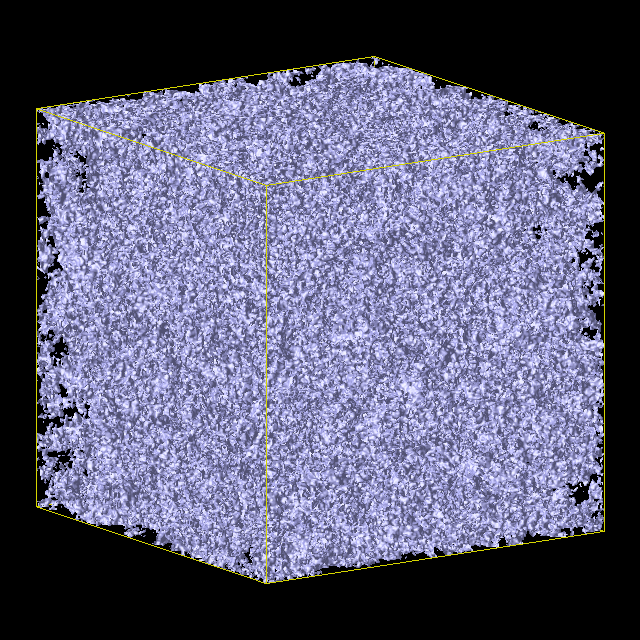
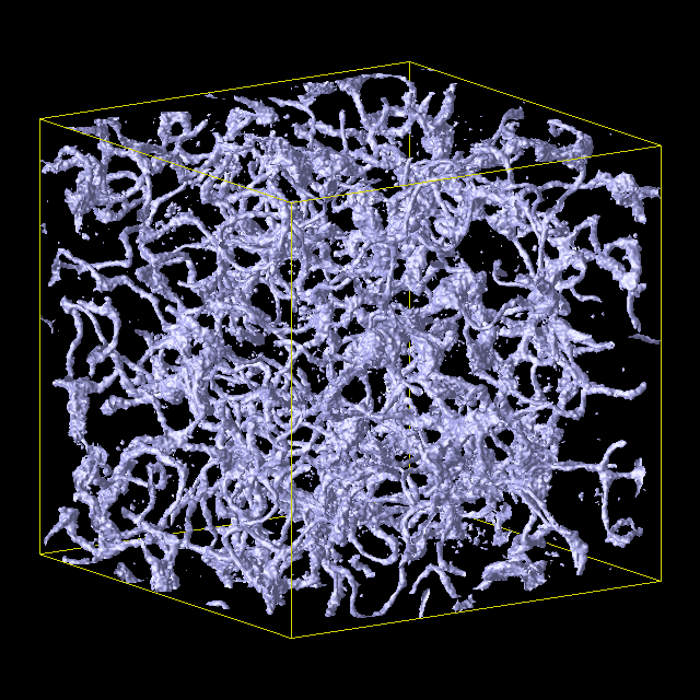
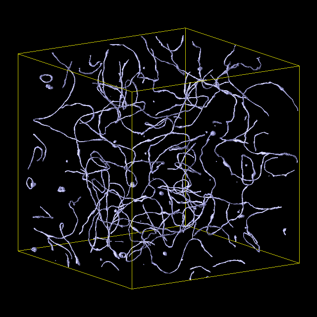
Figure 1: The isosurfaces with $|\varphi|=0.5\eta$ at $\tau\eta=5.45,\;6.27$ and $11.53$ for the simulation with $\lambda=1.0$ and $\beta=0.2$.

V.2 String energy

Next we identify all strings at each time step, and calculate their energies to check whether the string network is in the scaling regime. To calculate their energies, we do not use the string core identification technique discussed in Sec. IV.1 since it is difficult to set the string width which changes in time, and it does not matter where the string core is. Instead, we fix $\varphi_{c}$, and we identify the region satisfying $|\varphi|<\varphi_{c}$ as strings. Then the string energy is given by Eq. (22).

In Fig. 2, we show the time evolution of the string energy for $\beta=0.2$ and $\lambda=1.0$ with $\varphi_{c}=0.5\eta$ and $\varphi_{c}=0.2\eta$. For $\tau\eta\gtrsim 6.5$, we find that the relation $\rho_{\rm str}\propto\tau^{-4}$ is approximately satisfied at the late time, if we average the oscillatory behavior, and that the transition time seems insensitive to the choice of $\varphi_{c}$. This observation indicates that the network would lie in the scaling regime.

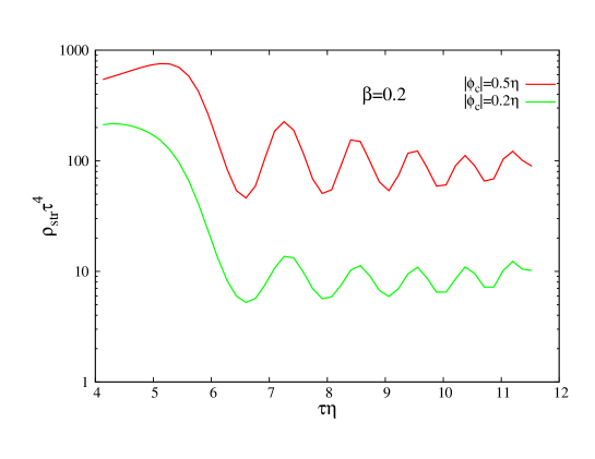
Figure 2: Time evolution of the string energy for $\beta=0.2$ and $\lambda=1.0$. The red line and green line correspond to $\varphi_{c}=0.5\eta$ and $\varphi_{c}=0.2\eta$, respectively.

V.3 Correlation length

In Fig. 3, we show the time evolution of the correlation length estimated by Eq. (18) for various values of $\beta$ including weakly Type-II regime with $\lambda=1.0$. Each of them is the average of 10 realizations, and the error bars indicate one $\sigma$. We found that the correlation length is strongly dependent upon $\beta$, particularly for $\beta<1.0$.

Our findings are as follows. First, the time of the start of the string formation is common to all the cases and is about $\tau\eta\approx 6.5$. Moreover, there is a general tendency that the correlation length $\xi$ becomes smaller. For $0.8\leq\beta\leq 1.4$, $\xi|_{\tau\eta\approx 6.5}$ becomes smaller, which indicates the initial density of the string network would be larger. For $0.4\leq\beta\leq 0.8$, $\xi|_{\tau\eta\approx 6.5}$ does not change so much, but the increasing rate of $\xi$, or $d\xi/d\tau$, becomes smaller as $\beta$ approaches $0.4$. Finally, as $\beta$ goes below $0.4$, $\xi|_{\eta\tau\approx 6.5}$ rises again while the low increasing rate is maintained.

The simulation results imply that the network with the smaller value of $\beta$ tends to take a smaller $\xi$, or be denser in the comoving box. To see this fact from another aspect, we calculate the effective number of strings in a virtual box whose volume is $\mathcal{H}^{-3}$, which hereafter we refer to as “horizon-sized box.” Focusing on a string, it occupies an area $\xi^{2}$ on the surface perpendicular to the string by definition. Hence, considering a cross-sectional surface of the simulation box, one can imagine that $\mathcal{H}^{-2}/\xi^{2}$ strings pass across the surface. According to this naive expectation, we estimate the effective number of strings in the horizon-sized box by

$$N_{\rm eff}=\frac{1}{\mathcal{H}^{2}\xi^{2}}.$$ (23)

If $\xi$ behaves approximately as $\xi(\tau)=c\tau+\xi_{0}$ where $c$ and $\xi_{0}$ are constants and we neglect the oscillatory behavior, $N_{\rm eff}$ at the late time becomes

$$N_{\rm late}=\lim_{\tau\to\infty}N_{\rm eff}=\frac{1}{c^{2}},$$ (24)

where we used $\mathcal{H}=1/\tau$ in the radiation-dominant Universe. This equation indicates that the network density in the horizon-sized box is determined by the increasing rate of $\xi$, and also the correspondence to the fact that the number of strings in the horizon-sized box is constant in the scaling regime. We estimate the ensemble average, $\langle c\rangle$, using the data obtained by all realizations, and then we obtain the late-time number of strings in the simulation box, $N_{\rm late}$.

The details of the procedure to obtain $N_{\rm late}$ are explained in Appendix C. Briefly speaking, we first remove the oscillatory behavior of $\xi$ in each realization, and then using the least-square method, we fit the data in the range of $\tau_{\rm start}\leq\tau\leq\tau_{\rm end}$ to the ansatz $\xi=c\tau+\xi_{0}$ where $\tau_{\rm start}\eta=6.5$ and $\tau_{\rm end}$ is dependent on the value of $\beta$. How to choose $\tau_{\rm end}$ is discussed in Appendix A.

Figure 4 shows $N_{\rm late}$ against $\beta$. The error bars are due to the variation of $c$ in each realization. We found that $N_{\rm late}$ becomes obviously larger for $\beta<0.8$, while it is almost constant and only a few strings exist for $\beta\geq 0.8$. Although $\beta=0.4$ realized the maximum number of strings, it might be premature to conclude that the network with $\beta=0.4$ becomes densest in the horizon-sized box. As discussed in Appendix A, the reliable range of simulation data for $\beta<0.4$ is relatively short. In order to extend the reliable range, many more spatial resolutions are required to resolve the steep change of the gauge field around the string core, indicated by $m_{A}\to\infty$ for $\beta\to 0$, as discussed in Appendix B.

Back to the network density in the comoving box, we performed additional simulations for $q=0.11$ and $0.091$ with fixed $\gamma$ where $q$ is defined in Sec. III, and check whether the critical value of $\beta$ realizing the densest network in the comoving box depends on $q$. For the large value of $q$, the phase transition takes place at the earlier Universe since the transition temperature is given by $T_{c}=\sqrt{3}\eta=\sqrt{3}q\gamma M_{\rm pl}$. In Fig. 5, the phase transition at higher energies with $q=0.11$ provides a smaller critical $\beta$ around $0.2$, whereas the critical $\beta$ is not so clear for $q=0.091$, but would be around $0.8$. These facts imply that the string network density in the comoving box is strongly related to the dragging effect by the cosmic expansion.

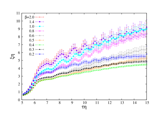
Figure 3: Time evolution of the correlation length estimated by Eq. (18).

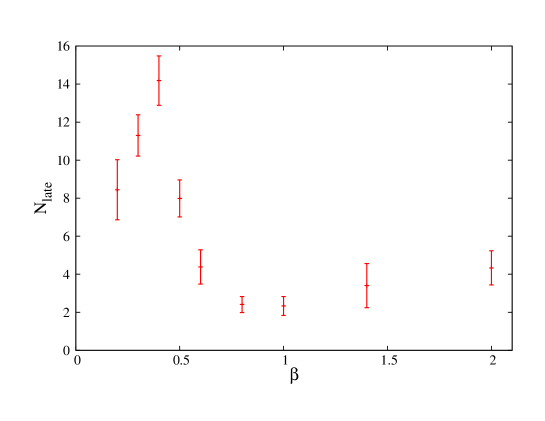
Figure 4: The effective number of strings in a horizon-sized box at the late time defined in Eq. (24). The error bars are originated from the variation of $c$ and the increasing rate of $\xi$ for each realization.

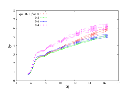
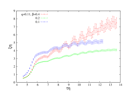
Figure 5: The correlation length with $q=0.091$ (left) and $q=0.11$ (right). A lower energy scale of the phase transition (left) results in a larger critical value of $\beta$ realizing the smallest $\xi$. In the present case, $q=0.091$ provides the critical $\beta$ between $0.6$ and $1.0$, whereas a higher phase transition with $q=0.11$ provides a smaller critical $\beta\sim 0.2$.

V.4 PRS algorithm

Finally, we investigate the effect of the PRS algorithm, given in Eq. (17), on the correlation lengths of the simulated Type-I string network. We choose $\beta=0.2$ and $0.4$, and also $\beta=1.0$ as a reference. Their correlation lengths are shown in Fig. 6. In this figure, we also plotted the corresponding results shown in Fig. 3. As we mentioned before, there is a strong dependence of $\xi$ on the value of $\beta$. In contrast, if we use the PRS algorithm, the $\beta$ dependence completely disappears, and thus it seems that we can obtain the universal value of the gradient of $\xi$ and $N_{\rm late}$.

Focusing on the case with the critical coupling (red line), the gradient of $\xi$ is almost insensitive to whether we use the PRS or not. This feature has been expected since there would be no interactions, or sufficiently weak, between strings in this case, except at the impact points of the reconnection process. Therefore, even if we vary the value of the coupling constants $\lambda$ and $e$ in time, the characteristics of the whole network are not so affected.

In contrast, this is not the case with the Type-I strings, which have the intrinsic string-string interactions. To use the PRS algorithm for them corresponds to weakening the interactions on purpose as time proceeds. Hence, the network would lack its characteristics depending on the value of $\beta$. Consequently, we would like to claim the need to carefully apply the PRS algorithm to the cases, except those with the critical coupling. Note that, for those with the PRS, the scaling regime starts later than those without the PRS. This is because $\lambda$ is decreased at and after the phase transition. Smaller $\lambda$ means that the potential becomes more flat and thus it takes more time for the field to sufficiently relax and then to satisfy $V(\varphi;T)<V(0;T)$.

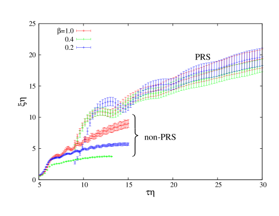
Figure 6: The correlation length of simulated string network with and without the PRS algorithm.

VI Conclusion and discussion

We numerically studied the formation and time evolution of Type-I cosmic-string networks in the Abelian-Higgs model by three-dimensional lattice simulations in a box with $N=1024^{3}$ grid. Figure 2 was useful to check that the network actually enters the scaling regime. Then we particularly focused on the dependence of the correlation length $\xi$ on the parameter $\beta$. In the Type-I regime ($\beta<1$), the gauge field plays an important role for the interaction between strings. As seen in Fig. 3, we found that the time dependence of the correlation length is strongly dependent on the value of $\beta$. More concretely, we found that there seems to be a critical value of $\beta$ with which the string network becomes densest in the expanding Universe, and that this critical value becomes smaller, if the energy scale of the phase transition becomes higher; see Fig. 5. Furthermore, we found that the effective number of strings in a box with the volume $\mathcal{H}^{-3}$, as defined in Eq. (23), is almost constant for $\beta\gtrsim 0.8$, and the number tends to suddenly increase for $\beta\lesssim 0.8$; see Fig. 4. The figure also indicates that the number of strings has a peak at $\beta=0.4$. However, it would be premature to conclude that $\beta=0.4$ actually realizes the densest network since the reliable range of simulation data is not sufficiently wide due to the shortage of the spatial resolution of our simulations for $\beta<0.4$.

The critical value of $\beta$ seems to depend on the energy scale of the phase transition. We found that the phase transition at higher energies provides a smaller critical $\beta$, whereas the value becomes larger if the phase transition takes place at lower energies. This fact implies that the critical $\beta$ realizing the densest network is determined not only from the strength of the gauge interaction, but also from the environmental effect, namely, the cosmic expansion. In order to clarify the origin of the critical $\beta$, it would be needed to deeply investigate the string-string interaction in the Friedmann background.

So far, field-theoretic simulations of string network formation have been performed with the Press-Ryden-Spergel (PRS) algorithm where $\lambda$ and $e$ are varied in time to maintain the constancy of the comoving width of a string. This algorithm is effective for the lattice simulations in the expanding Universe since the expanding lattice spacing can forever, in principle, follow the width of the strings. In order to investigate the validity of this algorithm for the Type-I strings, we have also performed the simulations with the PRS algorithm. As a result, the interesting properties mentioned above completely disappeared, and hence we cannot find any differences among the results with different values of $\beta$. This result indicates that the PRS algorithm should not be applied to Type-I strings, if one focuses on the epoch soon after the phase transition where the string-string interaction would be strong.

However, there is a subtlety in the connection between the two results with and without the PRS algorithm in Fig. 6. Naively thinking, we can speculate that, at the sufficiently late time, the mean separation of the strings would become large enough for them to terminate the interactions with each other. This fact would mean that the correlation length evolves along with the results with the PRS algorithm shown in Fig. 6 at the late time, since the change of string width must be negligible at the sufficiently late time. In other words, it is expected that the gradient of $\xi$ without the PRS would become larger at some time when the string-string interaction can be neglected, and then the gradient becomes similar to that with the PRS. Unfortunately, with our present computer resources, we could not follow the simulations up to such a transition point, and thus this is still an open question.

Appendix A Convergence check of numerical results

We check the robustness of our numerical results to the resolution. Figure 7 shows that the correlation length with $\beta=0.2$, 0.4 and 0.8 when we vary the number of grids with a fixed box size, $L$. In the comoving coordinate, a string seems to become thinner in time, and thus the simulation is broken down when the grid can no longer resolve the string. This fact reflects that the end time of each simulation becomes later as $N$ is increased. Moreover, just before the breakdown, $\xi$ tends to be flat, while it grew almost linearly. Therefore, the reliable results would be obtained only in the region where two results with different resolutions overlap.

Due to this shortage of resolutions at the late time, we use only the relatively reliable part of simulation data in the finite time range, $\tau_{\rm start}\leq\tau\leq\tau_{\rm end}$, when we estimate the gradient of $\xi$ in Sec. V.3 or Appendix C. For all cases, we fix $\tau_{\rm start}=6.5\eta^{-1}$ corresponding to the starting time of the scaling regime, and basically $\tau_{\rm end}=15\eta^{-1}$ which is the end time of simulations. From the results in Fig. 7, we choose $\tau_{\rm end}=13\eta^{-1}$ for $\beta=0.4$, and $\tau_{\rm end}=12\eta^{-1}$ for $\beta=0.2$.

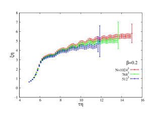
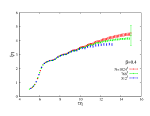
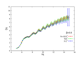
Figure 7: The resolution dependence of the estimated correlation length with $\beta=0.2$ (left), $\beta=0.4$ (center) and $\beta=0.8$ (right). We fixed the box size, $L$, and varied the grid size as $N=1024^{3}$ (red), $768^{3}$ (green) and $512^{3}$ (blue).

Appendix B Static vortex width

Consider the axial-symmetric string configuration in the Minkowski spacetime, so-called Abrikosov-Nielsen-Olesen vortex Abrikosov:1956sx ; Nielsen:1973cs . According to Ref. Vilenkin , using the cylindrical coordinates $(r,\theta,z)$ that originated from the center of the string, the scalar field and the gauge field can be represented by the following forms:

$$\varphi(\mathbf{x}) =\eta e^{in\theta}f(r),$$ (25)

$$A_{\theta}(\mathbf{x}) =\frac{n}{e}\alpha(r),\qquad A_{r}=A_{z}=0,$$ (26)

where $n$ is the winding number of the string. Substituting them into Eqs. (4) and (5) with $g_{\mu\nu}={\rm diag}(-1,1,r^{2},1)$, and neglecting the time dependence, the governing equations for $f(r)$ and $\alpha(r)$ are given by

$$\frac{d^{2}f}{d\hat{r}^{2}}+\frac{1}{\hat{r}}\frac{df}{d\hat{r}}-\frac{n^{2}f}{\hat{r}^{2}}(\alpha-1)^{2}-\lambda f(f^{2}-1)=0,$$ (27)

$$\frac{d^{2}\alpha}{d\hat{r}^{2}}-\frac{1}{\hat{r}}\frac{d\alpha}{d\hat{r}}-2e^{2}f^{2}(\alpha-1)=0,$$ (28)

where $\hat{r}=r\eta$ and we neglect the temperature-dependent terms in the potential $V(\varphi)$. The boundary conditions are given as $f(r),\alpha(r)=0$ for $r=0$ and $f(r),\alpha(r)\to 1$ for $r\to\infty$. With these conditions, we solved the above equations numerically. Then we calculated the half-value widths of $f(r)$ and $\alpha(r)$, the value of $r$ satisfying $f(r)=1/2$ or $\alpha(r)=1/2$, for the various $\beta$ as the estimator of the string width. Figure 8 shows the $\beta$ dependence of the half-value widths for $n=1$ strings with $\lambda=1.0$. Clearly the string cores consisting of the scalar field and the gauge field get thin for Type-I strings ($\beta<1$). In other words, the large $e$ with a fixed value of $\lambda$ or the small $\lambda$ with a fixed value of $e$ produces thin strings. In particular, the half-value width of the gauge field is more strongly dependent on $\beta$ than that of the scalar field. This property requires the finer resolution of the computational domain, particularly for $\beta<1$.

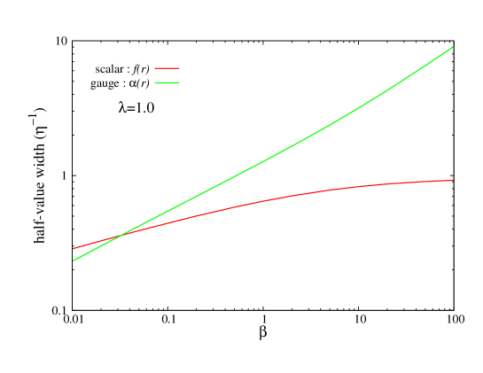
Figure 8: The $\beta$ dependence of the half-value width of functions $f(r)$ and $\alpha(r)$ for $n=1$ strings with $\lambda=1.0$.

Appendix C Estimation of gradient of $\xi$, and $N_{\rm late}$

The following is the flow chart to estimate $N_{\rm late}$ defined in Eq. (24) from the raw simulation data of $\xi$ shown in Fig. 3.

• Determining the reliable range of $\xi$ data, $\tau_{\rm end}$, discussed in Appendix A.

• Smoothing $\xi$ to remove the oscillatory behavior.

• Fitting each smoothed $\xi$ to a linear function of $\tau$ to obtain the gradient of $\xi$, and averaging all realizations to obtain the expectation value of the gradient and its variance.

First of all, according to the convergence check against the spatial resolution discussed in Appendix A, we determined the reliable range of $\xi(\tau)$ data, $\tau_{\rm end}$. Next, let us consider the smoothing process for the raw data of $\xi(\tau)$ containing the oscillations. Our final goal is to fit $\xi$ to a linear function such as $\xi(\tau)=c\tau+\xi_{0}$. Hence the smoothing process should not affect the gradient $c$. The simplest treatment would be the averaging with neighbor points in the time domain. Defining $\xi_{i}\equiv\xi(\tau_{i})$ for $i=1\ldots N$ and $\tau_{1}=\tau_{\rm start},\tau_{N}=\tau_{\rm end}$, this averaging can be described as

$$\xi_{1}={\rm fixed},\qquad\xi_{i}^{(j+1)}=\frac{\xi_{i-1}^{(j)}+\xi_{i+1}^{(j)}}{2},\qquad\xi_{N}={\rm fixed},$$ (29)

where $\xi_{i}^{(j)}$ represents the $j$ th smoothed data, and $\xi_{i}^{(0)}$ is the original raw data. We repeat this process until $j\leq j_{\rm max}$. This formula can be derived by approximating the equation $d^{2}\xi/d\tau^{2}|_{\tau=\tau_{i}}=0$ with the second-order central difference formula.

In Fig. 9, the blue line represents the resultant smoothed $\xi$ with $j=5$ times iterations, while the red line represents the original data. It is clear that only the oscillatory behaviors are successfully removed, and the global gradient does not change during this process.

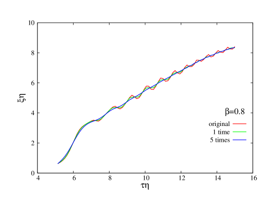
Figure 9: The red line is the original data of $\xi(\tau)$ for $\beta=0.8$. The green and blue lines are the resultant smoothed data with one time iteration and five times iterations, respectively.

Finally, we fit the linear regime of the smoothed $\xi$ in $\tau_{\rm start}\leq\tau\leq\tau_{\rm end}$ to a linear function, $\xi(\tau)=c\tau+\xi_{0}$. According to this procedure, we obtain ten independent values of $c$ from the ten sets of simulation data for a given $\beta$. Then we can calculate the expectation value of $c$, $\langle c\rangle$, and its variance, $\sigma_{c}^{2}$. Finally, using the definition of $N_{\rm late}$ given in Eq. (24), we plot Fig. 4, where the error bar indicates $\sigma_{\xi}=|\partial N_{\rm late}/\partial c|\sigma_{c}=2\sigma_{c}/c^{3}$.

References

- (1) T. Damour and A. Vilenkin, Phys. Rev. Lett. 85 (2000) 3761 [gr-qc/0004075].
- (2) T. Damour and A. Vilenkin, Phys. Rev. D 64 (2001) 064008 [gr-qc/0104026].
- (3) T. Damour and A. Vilenkin, Phys. Rev. D 71 (2005) 063510 [hep-th/0410222].
- (4) X. Siemens, V. Mandic and J. Creighton, Phys. Rev. Lett. 98 (2007) 111101 [astro-ph/0610920].
- (5) X. Siemens, J. Creighton, I. Maor, S. Ray Majumder, K. Cannon and J. Read, Phys. Rev. D 73 (2006) 105001 [gr-qc/0603115].
- (6) B. P. Abbott et al. [LIGO Scientific Collaboration], Phys. Rev. D 80 (2009) 062002 [arXiv:0904.4718 [astro-ph.CO]].
- (7) B. P. Abbott et al. [LIGO Scientific and VIRGO Collaborations], Nature 460 (2009) 990 [arXiv:0910.5772 [astro-ph.CO]].
- (8) S. Olmez, V. Mandic and X. Siemens, Phys. Rev. D 81 (2010) 104028 [arXiv:1004.0890 [astro-ph.CO]].
- (9) S. Kuroyanagi, K. Miyamoto, T. Sekiguchi, K. Takahashi and J. Silk, Phys. Rev. D 86 (2012) 023503 [arXiv:1202.3032 [astro-ph.CO]].
- (10) N. Bevis, M. Hindmarsh, M. Kunz and J. Urrestilla, Phys. Rev. Lett. 100 (2008) 021301 [astro-ph/0702223].
- (11) K. Takahashi, A. Naruko, Y. Sendouda, D. Yamauchi, C. -M. Yoo and M. Sasaki, JCAP 0910 (2009) 003 [arXiv:0811.4698 [astro-ph]].
- (12) D. Yamauchi, K. Takahashi, Y. Sendouda, C. -M. Yoo and M. Sasaki, Phys. Rev. D 82 (2010) 063518 [arXiv:1006.0687 [astro-ph.CO]].
- (13) D. Yamauchi, Y. Sendouda, C. -M. Yoo, K. Takahashi, A. Naruko and M. Sasaki, JCAP 1005 (2010) 033 [arXiv:1004.0600 [astro-ph.CO]].
- (14) R. Battye and A. Moss, Phys. Rev. D 82 (2010) 023521 [arXiv:1005.0479 [astro-ph.CO]].
- (15) D. Yamauchi, K. Takahashi, Y. Sendouda and C. -M. Yoo, Phys. Rev. D 85 (2012) 103515 [arXiv:1110.0556 [astro-ph.CO]].
- (16) C. Dvorkin, M. Wyman and W. Hu, Phys. Rev. D 84 (2011) 123519 [arXiv:1109.4947 [astro-ph.CO]].
- (17) J. Urrestilla, N. Bevis, M. Hindmarsh and M. Kunz, JCAP 1112 (2011) 021 [arXiv:1108.2730 [astro-ph.CO]].
- (18) S. Kuroyanagi, K. Miyamoto, T. Sekiguchi, K. Takahashi and J. Silk, Phys. Rev. D 87 (2013) 023522 [arXiv:1210.2829 [astro-ph.CO]].
- (19) P. A. R. Ade et al. [Planck Collaboration], arXiv:1303.5085 [astro-ph.CO].
- (20) A. Vilenkin and E. P. S. Shellard, Cambridge University Press, 1994.
- (21) A. A. Fraisse, C. Ringeval, D. N. Spergel and F. R. Bouchet, Phys. Rev. D 78 (2008) 043535 [arXiv:0708.1162 [astro-ph]].
- (22) G. R. Vincent, M. Hindmarsh and M. Sakellariadou, Phys. Rev. D 56 (1997) 637 [astro-ph/9612135].
- (23) A. Albrecht and N. Turok, Phys. Rev. D 40 (1989) 973.
- (24) A. Albrecht and N. Turok, Phys. Rev. Lett. 54 (1985) 1868.
- (25) D. P. Bennett and F. R. Bouchet, Phys. Rev. D 41 (1990) 2408.
- (26) B. Allen and E. P. S. Shellard, Phys. Rev. Lett. 64 (1990) 119.
- (27) C. J. A. P. Martins and E. P. S. Shellard, Phys. Rev. D 73 (2006) 043515 [astro-ph/0511792].
- (28) K. D. Olum and V. Vanchurin, Phys. Rev. D 75 (2007) 063521 [astro-ph/0610419].
- (29) C. Ringeval, M. Sakellariadou and F. Bouchet, JCAP 0702 (2007) 023 [astro-ph/0511646].
- (30) J. J. Blanco-Pillado, K. D. Olum and B. Shlaer, Phys. Rev. D 83 (2011) 083514 [arXiv:1101.5173 [astro-ph.CO]].
- (31) G. Vincent, N. D. Antunes and M. Hindmarsh, Phys. Rev. Lett. 80 (1998) 2277 [hep-ph/9708427].
- (32) J. N. Moore, E. P. S. Shellard and C. J. A. P. Martins, Phys. Rev. D 65 (2001) 023503 [hep-ph/0107171].
- (33) N. Bevis, M. Hindmarsh, M. Kunz and J. Urrestilla, Phys. Rev. D 75 (2007) 065015 [astro-ph/0605018].
- (34) P. Mukherjee, J. Urrestilla, M. Kunz, A. R. Liddle, N. Bevis and M. Hindmarsh, Phys. Rev. D 83 (2011) 043003 [arXiv:1010.5662 [astro-ph.CO]].
- (35) N. Bevis, M. Hindmarsh, M. Kunz and J. Urrestilla, Phys. Rev. D 82 (2010) 065004 [arXiv:1005.2663 [astro-ph.CO]].
- (36) L. M. A. Bettencourt and R. J. Rivers, Phys. Rev. D 51 (1995) 1842 [hep-ph/9405222].
- (37) L. M. A. Bettencourt, P. Laguna and R. A. Matzner, Phys. Rev. Lett. 78 (1997) 2066 [hep-ph/9612350].
- (38) P. Salmi, A. Achucarro, E. J. Copeland, T. W. B. Kibble, R. de Putter and D. A. Steer, Phys. Rev. D 77 (2008) 041701 [arXiv:0712.1204 [hep-th]].
- (39) S. Sarangi and S.-H. H. Tye, Phys. Lett. B 536, 185 (2002) [arXiv:hep-th/0204074].
- (40) N. T. Jones, H. Stoica and S.-H. H. Tye, Phys. Lett. B 563, 6 (2003) [arXiv:hep-th/0303269].
- (41) E. J. Copeland, R. C. Myers and J. Polchinski, JHEP 0406, 013 (2004) [arXiv:hep-th/0312067].
- (42) G. Dvali and A. Vilenkin, JCAP 0403, 010 (2004) [arXiv:hep-th/0312007].
- (43) J. Urrestilla and A. Vilenkin, JHEP 0802 (2008) 037 [arXiv:0712.1146 [hep-th]].
- (44) A. Achucarro and R. de Putter, Phys. Rev. D 74 (2006) 121701 [hep-th/0605084].
- (45) M. Yamaguchi, Phys. Rev. D 60 (1999) 103511 [hep-ph/9907506].
- (46) M. Yamaguchi and J. Yokoyama, Phys. Rev. D 66 (2002) 121303 [hep-ph/0205308].
- (47) M. Yamaguchi and J. Yokoyama, Phys. Rev. D 67 (2003) 103514 [hep-ph/0210343].
- (48) U.-L. Pen, U. Seljak and N. Turok, Phys. Rev. Lett. 79 (1997) 1611 [astro-ph/9704165].
- (49) R. Durrer, M. Kunz and A. Melchiorri, Phys. Rev. D 59 (1999) 123005 [astro-ph/9811174].
- (50) M. Yamaguchi, J. Yokoyama and M. Kawasaki, Phys. Rev. D 61 (2000) 061301 [hep-ph/9910352].
- (51) M. Yamaguchi, M. Kawasaki and J. Yokoyama, Phys. Rev. Lett. 82 (1999) 4578 [hep-ph/9811311].
- (52) Y. Cui, S. P. Martin, D. E. Morrissey and J. D. Wells, Phys. Rev. D 77 (2008) 043528 [arXiv:0709.0950 [hep-ph]].
- (53) M. Hindmarsh, S. Stuckey and N. Bevis, Phys. Rev. D 79 (2009) 123504 [arXiv:0812.1929 [hep-th]].
- (54) W. H. Press, B. S. Ryden and D. N. Spergel, Astrophys. J. 347 (1989) 590.
- (55) A. A. Abrikosov, Sov. Phys. JETP 5 (1957) 1174 [Zh. Eksp. Teor. Fiz. 32 (1957) 1442].
- (56) H. B. Nielsen and P. Olesen, Nucl. Phys. B 61 (1973) 45.