Quartic quasi-topological gravity, black holes and holography

Abstract

In this paper, we derive the field equations of quartic quasi-topological gravity by varying the action with respect to the metric. Also, we obtain the linearized graviton equations in the AdS background and find that it is governed by a second-order field equation as in the cases of Einstein, Lovelock or cubic quasi-topological gravities. But in contrast to the cubic quasi-topological gravity, the linearized field equation around a black hole has fourth-order radial derivative of the perturbation. Moreover, we analyze the conditions of having ghost free AdS solutions and AdS planar black holes. In addition, we compute the central charges of the dual conformal field theory of this gravity theory by studying holographic Weyl anomaly. Finally, we consider the effect of quartic term on the causality of dual theory in the tensor channel and show that, in the contrast to the trivial result of cubic quasi-topological gravity, the existence of both cubic and quartic terms leads to a non-trivial constraint. However, this constraint does not imply any lower positive bound on the viscosity/entropy ratio.

1 Introduction

The anti-de Sitter/conformal field theory (AdS/CFT) correspondence provides an interesting framework to study the non-perturbative quantum field theories. This kind of duality for the first time introduced in the context of string theory. However, the most strong version of this conjecture is generalized to gauge/gravity duality independent of string theory consideration. According to this duality, in principle, one can perform gravity calculation to find information about the field theory side or vice versa AdS . As a simple model in the context of AdS/CFT, one can consider Einstein gravity with a two-derivative bulk action. But in this circumstance, the dual theory is restricted to the large N and large ‘t Hooft couplings. Moreover, the central charges of a conformal field theory (CFT) relate to coupling constants of its dual gravity. Therefore, Einstein gravity restricts dual theory to limited class of CFT with equal central charges CentCharg1 . In order to extend the duality beyond these limits, one needs to involve higher curvature terms or derivatives of curvature tensor in the gravity action. It is clear that each correction term introduces a new coupling constant and so this procedure leads to the extension of parameter space and central charges and richness of the CFT theory CentCharg2 ; FinCoup ; Hofman . It is natural to take the correction terms which arises from a UV complete theory such as string theory. However, considering some toy models may help us to learn more about the AdS/CFT duality.

Gauss-Bonnet (second order of Lovelock) term with quadratic interaction or in general, Lovelock terms in all the orders are well-known corrections which usually are added to Hilbert-Einstein action. Lovelock gravity has some interesting features. For example, it leads to second-order field equation Lovelock and so it has ghost free AdS solution GhostFree . However, because of topological features of Lovelock theory, Gauss-Bonnet term has no contribution in spacetimes less than five dimensions and third-order of Lovelock contributes in seven or higher-dimensional spacetimes. Thus, for studying four-dimensional field theory with a five-dimensional holographic dual, only Gauss-Bonnet term is accessible. Throughout the recent years, most of the interesting holographic aspects of Lovelock gravity, has been studied Liu ; de Bore1 ; Edelstein1 ; Edelstein2 ; GBd ; de Bore2 ; EdelsteinPaulos ; EdelsteinRev . It is known that the second order Lovelock gravity (Gauss-Bonnet gravity) admits supersymmetric extension Ozkan:2013uk , while all the higher-orders of this theory have only the necessary condition of supersymmetric extension susy ; EdelsteinPaulos . By these considerations and for studying the effects of cubic interaction in the non-supersymmetric gravity on the four-dimensional CFT dual, the cubic quasi-topological gravity has been constructed Myers1 . This toy model provides a second-order field equation for spherically symmetric spacetime and admits ghost free AdS vacuum and asymptotic AdS black hole solutions in five dimensions Myers1 ; Oliva ; Myers2 ; CubicQuasiBH ; CubicQuasiHolo . As mentioned in Ref. Myers2 , one expects that the quasi-topological gravity may create a better understanding of non-supersymetric holography and some constraints like causality bound Liu and positive energy restriction Hofman . In fact, in the supersymmetric models the positive energy constraint involves causality bound, so they do not imply independent bound on the parameters of theory Hofman ; de Bore1 ; Edelstein1 ; Edelstein2 ; GBd ; de Bore2 ; EdelsteinPaulos ; EdelsteinRev . Moreover, it has been shown that the causality constraint and positive energy bound do not match in general, particularly for theories with more than second derivative in the field equation Hofman . Practically, positive energy and causality constraints are interesting, for example, for studying the conjecture about the existence of a lower bound on the ratio of shear viscosity to entropy Liu ; Myers2 ; Kss . However, the cubic quasi-topological gravity interaction does not imply any causality bound Myers2 . So the question is: does higher-order quasi-topological gravity has the same trivial result? By this motivation a more interesting version of quasi-topological gravity with quartic curvature terms has been introduced in Ref. Dehghani1 . In this paper, we are interested in the studies of the effects of this quartic term on the conditions of existence of ghost free AdS spacetimes and planar AdS black holes. Moreover, we like to know some aspects of quartic interaction on the CFT₄ in context of AdS₅/CFT₄.

Outline of this paper is as follows: We begin with a review on the action of quartic-topological gravity in Sec. 2. In Sec. 3, we obtain the general form of fourth-derivatives field equations by varying the action with respect to the metric $g_{ab}$. Moreover, we use this field equation for a spherically symmetric spacetime in order to show that the general fourth-derivative equation reduce to a second-order field equation. Also, we find the quartic equation which its roots describes the planar AdS solutions and review the thermodynamics of these black holes. Then in Sec. 4, we show that the first-order perturbation around an AdS solution reduces to a second-order wave equation for graviton. By using this wave equation, we obtain the conditions of existence of a ghost free AdS solution. In Sec. 5, we review a few properties of general solutions of quartic equation. In Sec. 6, we obtain the constraints on the parameter space of quartic quasi-topological gravity for having ghost free AdS and planar AdS black hole. In Sec. 7, we will use the standard approach of AdS/CFT to compute the central charges of four-dimensional conformal field theory dual to the five-dimensional quartic quasi-topological gravity. Section 8 is devoted to the study of perturbation around a planar AdS black hole and the possibility of causality violation. Moreover, the necessary condition for preserving the causality condition in tensor channel is introduced. Finally in Sec. 9, we consider the causality constraint in order to find whether it can imply any positive bound on the viscosity/entropy ratio. We finish our paper with some concluding remarks.

2 Review of Quartic Quasi-topological Action in Five Dimensions

In this section, we review some features of the cubic and quartic quasi-topological gravity in a five-dimensional spacetime, which may be considered as the dual of a four-dimensional CFT. This theory of gravity produces second-order differential equations of motion for a spherical symmetric spacetime. The bulk gravity action in the presence of a cosmological constant can be written as:

$$I_{G}=\frac{1}{2l_{p}^{3}}\int d^{5}x\sqrt{-g}[\mathcal{L}_{1}+\frac{\lambda}{2}L^{2}\mathcal{L}_{2}+\frac{7}{4}\mu L^{4}\mathcal{L}_{3}+\frac{1}{21024}\nu L^{6}\mathcal{L}_{4}],$$ (1)

where $\mathcal{L}_{1}=R-2\Lambda$ and $\mathcal{L}_{2}=R_{abcd}{R}^{abcd}-4{R}_{ab}{R}^{ab}+{R}^{2}$ are the Einstein-Hilbert and Gauss-Bonnet terms, and $\mathcal{L}_{3}$ and $\mathcal{L}_{4}$ are the cubic and quartic terms of quasi-topological gravity, respectively Myers1 ; Dehghani1 :

$$\mathcal{L}_{3} = a_{1}R_{a\,\,b}^{\,\,c\,\,\,d}R_{c\,\,d}^{\,\,e\,\,\,f}R_{e\,\,f}^{\,\,a\,\,\,b}+a_{2}\,R_{abcd}R^{abcd}R+a_{3}\,R_{abcd}R^{abc}{}_{e}R^{de}$$

$$+a_{4}\,R_{abcd}R^{ac}R^{bd}+a_{5}R_{a}{}^{b}R_{b}{}^{c}R_{c}{}^{a}+a_{6}\,R_{a}^{\,\,b}R_{b}^{\,\,a}R+a_{7}\,R^{3}$$

$$\ \mathcal{L}_{4} = c_{1}R_{abcd}R^{cdef}R_{\phantom{hg}{ef}}^{hg}R_{hg}{}^{ab}+c_{2}R_{abcd}R^{abcd}R_{ef}R^{ef}+c_{3}RR_{ab}R^{ac}R_{c}{}^{b}+c_{4}(R_{abcd}R^{abcd})^{2}$$ (2)

$$+c_{5}R_{ab}R^{ac}R_{cd}R^{db}+c_{6}RR_{abcd}R^{ac}R^{db}+c_{7}R_{abcd}R^{ac}R^{be}R_{\phantom{d}{e}}^{d}+c_{8}R_{abcd}R^{acef}R_{\phantom{b}{e}}^{b}R_{\phantom{d}{f}}^{d}$$

$$+c_{9}R_{abcd}R^{ac}R_{ef}R^{bedf}+c_{10}R^{4}+c_{11}R^{2}R_{abcd}R^{abcd}+c_{12}R^{2}R_{ab}R^{ab}$$

$$+c_{13}R_{abcd}R^{abef}R_{ef}{}_{g}^{c}R^{dg}+c_{14}R_{abcd}R^{aecf}R_{gehf}R^{gbhd},$$

$$a_{1} = 1,\ a_{2}=\frac{3}{8},\ a_{3}=\frac{-9}{7},\ a_{4}=\frac{15}{7},\ a_{5}=\frac{18}{7},\ a_{6}=\frac{-33}{14},\ a_{7}=\frac{15}{56},$$

$$c_{1} = -1404,\text{ \ \ \ \ }c_{2}=1848,\text{ \ \ \ \ \ }c_{3}=-25536,\text{ \ \ \ }c_{4}=-7422,\text{ \ \ \ \ }c_{5}=24672,$$

$$c_{6} = -5472,\text{ \ \ }c_{7}=77184,\text{ \ }c_{8}=-85824{,}\text{ \ \ \ }c_{9}=-41472{,}\text{ \ \ }c_{10}=-690,$$

$$c_{11} = 1788,\text{ \ \ }c_{12}=6936,\text{ \ }c_{13}=7296{,}\text{ \ \ }c_{14}=42480.$$ (3)

As usual we define $\Lambda=-6/L^{2}$, where $L$ is related to $AdS_{5}$ radius.

3 Field Equation of Quartic Quasi-topological Gravity

Here, we will closely follow Ref. Padd to derive the field equation of quasi-topological gravity by varying the action with respect to the metric $g^{ab}$. Consider a general action

$$I=\int_{\mathcal{M}}d^{n+1}x\sqrt{-g}\left[\mathcal{L}_{g}(g^{ab},R_{bcd}^{a})+\kappa\mathcal{L}_{m}\right],$$ (4)

where $\mathcal{L}_{m}$ is the matter Lagrangian and $\mathcal{L}_{g}(g^{ab},R_{bcd}^{a})$ is a general gravitational Lagrangian, which contains the metric and Riemann tensors but not any derivatives of $R_{bcd}^{a}$. Variation of this action with respect to $g^{ab}$ leads to

$$\delta I = \int_{\mathcal{M}}d^{n+1}x\sqrt{-g}(\mathcal{E}_{ab}-\kappa T_{ab})~{}\delta g^{ab},$$ (5)

$$\mathcal{E}_{ab} = \frac{1}{\sqrt{-g}}\frac{\partial\sqrt{-g}\mathcal{L}_{g}}{\partial g^{ab}}-2\nabla^{m}\nabla^{n}P_{amnb}~{};~{}\ \ \ \ \ \ P_{a}^{~{}\ bcd}\equiv\frac{\partial\mathcal{L}_{g}}{\partial R_{\ bcd}^{a}},$$ (6)

where $T_{ab}$ is the energy momentum tensor of matter field. By considering $\partial\sqrt{-g}/\partial g^{ab}=-\sqrt{-g}g_{ab}/2$, one obtains

$$\frac{1}{\sqrt{-g}}\frac{\partial\sqrt{-g}\mathcal{L}_{g}}{\partial g^{ab}} = \frac{\partial\mathcal{L}_{g}}{\partial R_{ij}^{kl}}\frac{\partial R_{ij}^{kl}}{\partial g^{ab}}-\frac{1}{2}g_{ab}~{}\mathcal{L}_{g}$$ (7)

$$= P_{b}^{\ \ \ kij}R_{akij}-\frac{1}{2}g_{ab}~{}\mathcal{L}_{g}.$$

So, the field equation can be written as

$$P_{b}^{\ kij}R_{akij}\mathcal{-}2\nabla^{m}\nabla^{n}P_{amnb}-\frac{1}{2}g_{ab}~{}\mathcal{L}_{g}=\kappa T_{ab}.$$ (8)

To have an explicit form of the field equation, one needs to calculate $P_{abcd~{}\ }$in term of Riemann and metric tensor. In general, the field equation (8) contains fourth-order derivatives of the metric due to the existence of $\nabla^{m}\nabla^{n}P_{amnb}$. But for Einstein and any Lanczos-Lovelock Lagrangian $\nabla^{n}P_{amnb}=0$, and therefore the field equation (8) contains at most second-order derivatives of the metric.

Using standard software Cad , it is a matter of calculation to show that $P_{abcd}$ for the Lagrangian of quasi-topological gravity (2) is

$$P_{a}^{\ bcd}=P_{(1)a}^{\ \ \ \ bcd}+\frac{\lambda}{2}L^{2}P_{(2)a}^{\ \ \ \ bcd}+\frac{7}{4}\mu L^{4}P_{(3)a}^{\ \ \ \ bcd}+\frac{1}{21024}\nu L^{6}P_{(4)a}^{\ \ \ \ bcd},$$ (9)

where

$$P_{(i)abcd}^{\ \ \ \ }=\frac{1}{2}(\Pi_{(i)[ab][cd]}+\Pi_{(i)[cd][ab]}).$$ (10)

In Eq. (10), $\Pi_{(i)abcd}$’s are

$${\Pi}_{(1)a}\,^{bcd}=g_{a}^{c}g^{bd},\text{ \ \ \ }{\Pi}_{(2)a}\,^{bcd}=2R_{a}^{\ bcd}-8g_{a}^{c}R^{bd}+2g_{a}^{c}g^{bd}R,$$ (11)

$${\Pi}_{(3)a}\,^{bcd} = a_{1}(3R^{bmdn}R_{man}^{\ \ \ \ \ \ \ c})+a_{2}(2RR_{a}^{\ \ bcd}+R_{mnop}R^{mnop}g_{a}^{c}g^{bd})$$ (12)

$$+a_{3}(2R_{a}^{\ \ bcm}R_{m}^{d}+R^{mnod}R_{mno}^{\ \ \ \ \ \ \ b}g_{a}^{c})+a_{4}(2R^{bmdn}R_{mn}g_{a}^{c}+R_{a}^{c}R^{bd})$$

$$+a_{5}(3R_{a}^{m}R_{m}^{c}g^{bd})+a_{6}(2RR_{a}^{c}g^{bd}+R_{mn}R^{mn}g_{a}^{c}g^{bd})+a_{7}(3R^{2}g_{a}^{c}g^{bd}),$$

$${\Pi}_{(4)a}\,^{bcd} = c_{1}(2{R}^{mn}\,_{a}\,{}^{b}{R}_{mn}\,^{op}{R}^{cd}\,_{op}+2{R}^{mnop}{R}_{a}\,^{b}\,{}_{mn}{R}_{op}\,^{cd})$$ (13)

$$+c_{2}(2\,{R}_{a}\,^{bcd}{R}_{mn}{R}^{mn}+{2R}^{bd}{R}^{mnop}{R}_{mnop}{g}_{a}\,^{c}),$$

$$+c_{3}(R^{mn}R_{mo}R_{n}^{o}g_{a}^{c}g^{bd}+R_{am}R^{cm}Rg^{bd}+2g_{a}^{c}R^{bm}R_{m}^{d}R)+c_{4}(4{R}_{a}\,^{bcd}{R}^{mnop}{R}_{mnop})$$

$$+c_{5}(4\,{R}^{bm}{R}^{dn}{R}_{mn}{g}_{a}\,^{c})+c_{6}({R}^{no}{R}^{qr}{R}_{nqor}{g}_{a}\,^{c}{g}^{bd}+R{R}_{a}\,^{c}{R}^{bd}+2R{R}^{no}{R}^{b}\,_{n}\,{}^{d}\,_{o}{g}_{a}\,^{c})$$

$$+\,c_{7}({R}_{a}\,^{c}{R}^{bm}{R}^{d}\,_{m}+{R}^{mn}{R}_{m}\,^{p}{R}^{b}\,_{n}\,{}^{d}\,_{p}{g}_{a}\,^{c}+{R}^{dm}{R}^{op}{R}_{o}\,^{b}\,{}_{pm}{g}_{a}\,^{c}+{R}_{a}\,^{n}{R}^{pq}{R}_{pnq}\,^{c}{g}^{bd})$$

$$+c_{8}({R}^{bm}{R}^{dn}{R}_{a}\,^{c}\,{}_{mn}+{R}^{cm}{R}^{dn}{R}_{am}\,^{b}\,{}_{n}+{R}^{mn}{R}_{am}\,^{op}{R}_{o}\,^{c}\,{}_{pn}{g}^{bd}-{R}^{mn}{R}^{o}\,_{m}\,{}^{pc}{R}_{anop}{g}^{bd})$$

$$+c_{9}({R}_{a}\,^{c}{R}^{mn}{R}^{b}\,_{m}\,{}^{d}\,_{n}+2{R}^{mn}{R}_{m}\,^{o}\,{}_{n}\,^{p}{R}^{b}\,_{o}\,{}^{d}\,_{p}{g}_{a}\,^{c}+{R}^{bd}{R}^{no}{R}_{nao}\,^{c})+c_{10}(4R^{3}{g}_{a}\,^{c}{g}^{bd})$$

$$+c_{11}(2\,R{R}^{mnop}{R}_{mnop}{g}_{a}\,^{c}{g}^{bd}+2\,R^{2}{R}_{a}\,^{bcd})+c_{12}(2\,R{R}^{mn}{R}_{mn}{g}_{a}\,^{c}{g}^{bd}+2\,R^{2}{R}^{bd}{g}_{a}\,^{c})$$

$$+c_{13}(2{R}^{dm}{R}^{npc}\,_{m}{R}_{a}\,^{b}\,{}_{np}+{R}^{mn}{R}_{a}\,^{bp}\,{}_{m}{R}^{cd}\,_{pn}+{R}^{mnob}{R}^{pq}\,_{o}\,{}^{d}{R}_{mnpq}{g}_{a}\,^{c})$$

$$+c_{14}(4\,{R}_{a}\,^{mcn}{R}^{obpd}{R}_{monp}).$$

One can show that $\nabla^{n}P_{amnb}=0$ for static spacetimes (with flat, spherical or hyperbolic boundary) in the quartic quasi-topological gravity, and therefore the field equation is at most second-order differential equation.

3.1 Planar AdS Black Holes in 5 dimensions

The metric of a five-dimensional planar AdS static spacetime may be written as

$$ds^{2}=\frac{r^{2}}{L^{2}}(-N^{2}(r)f(r)dt^{2}+dx^{2}+dy^{2}+dz^{2})+\frac{L^{2}}{r^{2}f(r)}dr^{2}.$$ (14)

Using the field equations of quasi-topological gravity, one obtains

$$\frac{3}{2L^{4}r}N(r)^{2}f(r)[r^{4}(1-f+\lambda f^{2}+\mu f^{3}+\nu f^{4})]^{\prime}=0,$$ (15)

$$\frac{3}{2r^{5}f(r)}[r^{4}(1-f+\lambda f^{2}+\mu f^{3}+\nu f^{4})]^{\prime}$$

$$-\frac{3}{rN(r)}[1-2\lambda f-3\mu f^{2}-4\nu f^{3}]N(r)^{\prime}=0.$$ (16)

So, the metric functions must satisfy the following equations

$$\gamma(f)\equiv 1-f(r)+\lambda f^{2}(r)+\mu f^{3}(r)+\nu f^{4}(r)-\frac{r_{h}^{4}}{r^{4}}=0,$$ (17)

$$N^{\prime}(r)=0,$$ (18)

where the integration constant $r_{h}$ is the radius of black hole horizon. Moreover, the last equation shows that $N(r)$ is a constant which we set it $N(r)=f_{\infty}^{-1/2}$ to fix the speed of light on the boundary equal to one. The constant $f_{\infty}$ is determined by taking $r\rightarrow\infty$ (or equally $r_{h}\rightarrow 0$) limit of Eq. (17). Thus, it is one of the roots of the following quartic equation

$$\gamma(f_{\infty})\equiv 1-f_{\infty}+\lambda f_{\infty}^{2}+\mu f_{\infty}^{3}+\nu f_{\infty}^{4}=0.$$ (19)

One may note that the radius of the AdS vacuum solution is $L_{eff}=Lf_{\infty}^{-1/2}$ .

The black hole solutions of Eq. (17) have a horizon at $r=r_{h}$. The Hawking temperature of this horizon is given by

$$T=\frac{r_{h}}{\pi L^{2}\sqrt{f_{\infty}}}.$$ (20)

Moreover, the energy and entropy densities are

$$M=\frac{3r_{h}^{4}}{2l_{p}^{3}L^{5}\sqrt{f_{\infty}}},\ \ \ \ \ \ \ \ \ \ \ \ \ \ s=\frac{2\pi r_{h}^{3}}{l_{p}^{3}L^{3}},$$ (21)

and therefore as like as any natural 5-dimensional black hole duals to a thermal CFT₄, the relation between these quantities are $M=3Ts/4$.

4 Linearized Graviton Equation in the AdS₅ Vacuum

As we mentioned, the field equation of quasi-topological gravity for static spacetime is second-order differential equations. But, here we like to study the field equation under a small perturbation around the AdS₅ background. For cubic quasi-topological gravity, the authors of Ref. Myers1 examined the linearized equations of motion for a graviton perturbation, and showed that the linearized graviton equation in an AdS background is second-order. Here, we like to do the same job in quartic quasi-topological gravity. We examine the following trial perturbation around the AdS₅ background:

$$ds^{2}=\frac{r^{2}}{L^{2}}(-{dt^{2}}+dx^{2}+dy^{2}+dz^{2})+\frac{L^{2}}{f_{\infty}}\frac{dr^{2}}{r^{2}}+2\varepsilon h(t,r,x,z)dxdy+2\varepsilon k(t,r,x,z)dtdr.$$ (22)

Using Eq. (9), one finds that $\nabla^{m}\nabla^{n}P_{amnb}=0+O(\varepsilon^{2})$. For instance, the graviton equations $\mathcal{E}_{rt}$ and $\mathcal{E}_{xy}$ in the AdS background up to first order in $\varepsilon$ are

$$-\frac{\varepsilon}{2}f_{\infty}(1-2\lambda f_{\infty}-3\mu f_{\infty}^{2}-4\nu f_{\infty}^{3})\frac{L^{2}}{r^{2}}[\frac{\partial^{2}}{\partial x^{2}}h(t,r,x,z)+\frac{\partial^{2}}{\partial z^{2}}k(t,r,x,z)]=\kappa T_{rt},$$ (23)

$$-\frac{\varepsilon}{2}(1-2\lambda f_{\infty}-3\mu f_{\infty}^{2}-4\nu f_{\infty}^{3})\frac{1}{L^{2}r^{2}}[-L^{4}\frac{\partial^{2}}{\partial t^{2}}+r^{4}f_{\infty}\frac{\partial^{2}}{\partial r^{2}}$$

$$+r^{3}f_{\infty}\frac{\partial}{\partial r}+L^{4}\frac{\partial^{2}}{\partial z^{2}}-4r^{2}f_{\infty}]h(t,r,x,z)=\kappa T_{xy},$$ (24)

which show that the propagation of a graviton in an AdS background is governed by a second-order equation. $T_{ab}$, which has been added to the right-hand side of the field equation, is due to the minimally coupling of the metric and the matter field which creates the perturbation, or it can be taken into account for the higher order contributions in the graviton. Here, we should emphasize that we have tried various small perturbation around AdS₅ background to make sure that the above result is true for any first order perturbation. It seems that the above equations for a general small perturbation may be written in the same form as that of cubic quasi-topological gravity Myers1 ; Myers2 . That is

$$-\frac{1}{2}(1-2\lambda f_{\infty}-3\mu f_{\infty}^{2}-4\nu f_{\infty}^{3})[\nabla^{2}h_{ab}+\nabla_{a}\nabla_{b}h_{c}^{c}-\nabla_{a}\nabla^{c}h_{cb}-\nabla_{b}\nabla^{c}h_{ac}$$

$$+g_{(0)ab}(\nabla^{c}\nabla^{d}h_{cd}-\nabla^{2}h_{c}^{c})+\frac{2}{L_{eff}^{2}}(h_{ab}-g_{(0)ab}h_{c}^{c})]=\kappa T_{ab},$$ (25)

where $\nabla_{a}$ is the covariant derivative of the AdS₅ metric and $h_{ab}$ is the perturbation around the AdS₅ background $g_{(0)ab}$. This result up to an overall constant factor is the same as the propagation of a graviton in the AdS₅ background of the Einstein’s theory of gravity ($\lambda=\mu=\nu=0$). However, one can think about the sign of this overall factor and compare it with Einstein case, to conclude that one has a ghost free theory (as like as Einstein theory) provided

$$-\gamma^{\prime}(f_{\infty})=1-2\lambda f_{\infty}-3\mu f_{\infty}^{2}-4\nu f_{\infty}^{3}>0.$$ (26)

If this condition is violated, the kinetic term in the action will be appeared with an opposite common sign. Moreover, we will see in the following sections that how this property relates to the positive mass assumption of the black hole solution and unitary condition of dual theory. The fact that gravitons propagating in an AdS background simply obey the same equation of motion as in the Einstein gravity plays an important role in the understanding of the holographic properties of cubic quasi-topological gravity Myers2 and quartic quasi-topological gravity introduced in Ref. Dehghani1 .

5 General Solutions of Quartic Equations

The most general form of a quartic equation is given by

$$f^{4}+af^{3}+bf^{2}+cf+d=0,$$ (27)

which admits four solutions as

$$f_{1} = \frac{1}{4}\left[-a-K-\sqrt{-(H+K^{2})+2\frac{G}{K}}\right],\ f_{2}=\frac{1}{4}\left[-a-K+\sqrt{-(H+K^{2})+2\frac{G}{K}}\right],$$

$$f_{3} = \frac{1}{4}\left[-a+K-\sqrt{-(H+K^{2})-2\frac{G}{K}}\right],\ f_{4}=\frac{1}{4}\left[-a+K+\sqrt{-(H+K^{2})-2\frac{G}{K}}\right],$$

where

$$K=\left[\frac{2^{7/3}(I+2^{-2/3}(\sqrt{-\Delta}-J)^{2/3})}{3(\sqrt{-\Delta}-J)^{1/3}}-\frac{H}{3}\right]^{1/2},$$

$$I=b^{2}+12d-3ac,~{}\ J=9b(ac+8d)-27(c^{2}+a^{2}d)-2b^{3},$$

$$G=a^{3}-4ab+8c,\ \ H=8b-3a^{2},\text{ \ \ }\Delta=4I^{3}-J^{2}.$$

As one may see in Ref. Math , the general reality conditions of these solutions can be determined by the signs of $G$, $H$, $\Delta$ and

$$\delta=3a^{4}-16a^{2}b+16ac+16(b^{2}-4d).$$

The nature of roots is as follows:

I. Two real and two complex roots: If $\Delta<0$, then there are two real and two complex roots.

II. Four real roots: If $\Delta>0,~{}\delta>0,~{}H<0$ , then all the four roots are real.

III. No real roots: If $\Delta>0,~{}\delta<0,~{}H<0~{}$or $\Delta>0,~{}H\geq 0$, then there exists no real root. In order to  find the complete analysis for the special cases where either of $\Delta$, $\delta$,$\ H$ or $G$ vanishes one can see Math .

6 Asymptotic AdS Black Hole Solutions

In this section, we study the conditions of existence of asymptotic AdS black hole solutions. Indeed, as we will see, the AdS spacetime and AdS black hole exist only in a limited region of the full parameter space.

6.1 Ghost Free AdS Solutions

As we mentioned before, the asymptotic AdS solution exists when the large $r$ limit of the quartic equation $\gamma(f)\equiv 1-f+\lambda f^{2}+\mu f^{3}+\nu f^{4}-r_{h}^{4}/r^{4}=0$ has positive real roots. That is, the quartic equation (19) should have positive real root. Indeed, the cases with $f_{\infty}<0$ relate to dS solutions. So, we should find the conditions on the parameters $\lambda,$ $\mu$ and $\nu$ that Eq. (19) admits positive real roots. Moreover, we are interested in ghost free theory and therefore these real positive roots should fulfil the ghost free condition (26). To see the effects of quasi-topological terms, we first limit our study in the absence of Gauss-Bonnet term ($\lambda=0$), and give some comments in the presence of Gauss-Bonnet term ($\lambda\neq 0$) at the end of this section. In the absence of Gauss-Bonnet term, the discriminant functions $\Delta,~{}\delta$, $H$ and $G$ reduce to

$$\Delta = [108(4\nu+\mu)^{3}-729(\nu+\mu^{2})^{2}]\nu^{-6},$$

$$\delta = \frac{3\mu^{4}}{\nu^{4}}-\frac{16\mu}{\nu^{2}}-\frac{64}{\nu},\ \ H=\frac{-3\mu^{2}}{\nu^{2}}<0,\text{ \ }G=\frac{\mu^{3}}{\nu^{3}}-\frac{8}{\nu}.$$ (28)

Using the fact that $\gamma(0)=1$ and the large-$x$ behavior of $\gamma(x)=1-x+\mu x^{3}+\nu x^{4}$, one can analyze the roots of $\gamma(f_{\infty})=0\$as follow. For $x\rightarrow\pm\infty$, the quartic term dominates, $\gamma(x)\approx\nu x^{4}$, and therefore the sign of $\nu$ determines the behavior of polynomials $\gamma(x)$ for asymptotic values $x\rightarrow\pm\infty$ . In addition, $H<0$. Thus, the analysis of the solutions is as follows:

I. For the case (I) discussed in previous section with two real and two complex roots, two cases happen.

a.$~{}\nu>0$: in this case the Vieta’s formulas $\Pi_{i=1}^{4}f_{\infty(i)}=1/\nu$ implies that the two real roots have the same signs. This is due to the fact that the two complex roots are conjugate and their product are positive. Therefore in this case, there are two AdS or two dS vacua where always one of the AdS solution is ghosty and the other is ghost free. However, one can check that for positive $\mu$, when $G<0$ the two roots are positive and for $G>0$ the two roots are negative. Moreover, for $\mu<0$ the roots are positive Math . In summary, there are one ghosty AdS and one ghost free AdS for $\mu<0$ and for $\mu>0$ with negative $G$.

b. $\nu<0$: by using the Vieta’s formulas, it is easy to see there are one AdS and one dS solution. In this case by considering the slope of $\gamma^{\prime}(f_{\infty})<0$ and the asymptotic behavior $f_{\infty}\rightarrow\pm\infty$, one finds that the AdS solution is ghost free.

II. For case (II) discussed in the previous section with four real roots, one may find from Fig. 1 that this case happens only when $\mu>0$. Again, two cases happen.

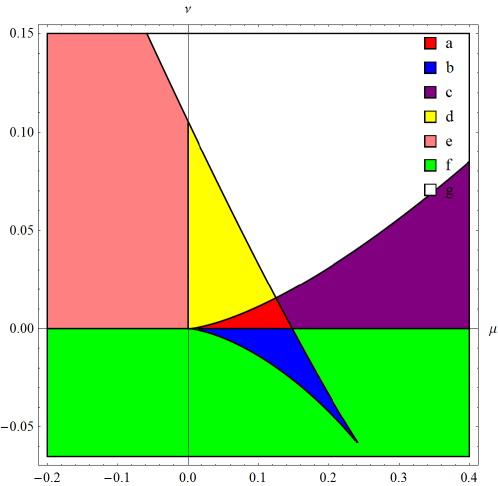
Figure 1: Regions (a) to (g) displayed in the parameter space $(\mu,\nu)$. There is no ghost free AdS in region (c). Moreover, the region (g) does not admit any AdS solution. See table 1 for more details about the other regions.

a. $\nu>0$: by using Vieta’s formulas $f_{\infty(1)}f_{\infty(2)}+f_{\infty(1)}f_{\infty(3)}+...+f_{\infty(3)}f_{\infty(4)}=\lambda/\nu=0$, one may see that it is not possible that all the roots have the same sign. In addition, $\gamma(0)=1$ and the asymptotic behavior $\gamma(f_{\infty})\approx\nu f_{\infty}^{4}~{}$ show there are two positive and two negative roots. So, in this case there are two dS solutions and two AdS where only one of the AdS solution is ghost free.

b. $\nu<0$: the Vieta’s formulas. $\Pi_{i=1}^{4}f_{\infty(i)}=1/\nu$ shows that the numbers of negative roots are odd. But, it is a matter of numerical analysis to show that it is not possible to have three negative roots. Thus there are three AdS solutions while only one of them is ghost free.

6.2 Ghost Free AdS Planar Black Holes

Now, we study the conditions of existence of AdS planar black holes. In order to have this kind of black hole, the metric function $f(r)$ must have a few properties. First, one may expect for large $r$ the metric function behaves as

$$f(r)=f_{\infty}-\frac{m}{r^{4}}+O(\frac{1}{r^{5}}),$$ (29)

where $m$ is related to the mass of black hole and should be positive. By substituting this expansion in Eq. (17) and using Eq. (19), one obtains

$$m=\frac{\gamma(f_{\infty})}{\gamma^{\prime}(f_{\infty})}r^{4}-\frac{r_{h}^{4}}{\gamma^{\prime}(f_{\infty})},$$ (30)

which shows that for a ghost free ($\gamma^{\prime}(f_{\infty})<0$) AdS black hole solution ($\gamma(f_{\infty})=0$), $m$ is positive. This fact relates the problem of negative mass to the problem of ghost in the AdS background.

Second, for an AdS black hole solution $f(r)$ must be a real monotonous increasing function in the domain $r\in(r_{\ast},\infty)$ from the negative value $f_{\ast}=f(r_{\ast})$ to $f_{\infty}>0$ (see Fig. (2)) . As we will show later, the spacetime is singular at $r_{\ast}$ and $f(r)$ is complex for the excluded region $r<r_{\ast}$ (see Fig. 2). In this case, $f(r)$ is zero at $r=r_{h}$ and therefore $f(r)$ describes a black hole solution. This shows that $f_{\infty}$ in Eq. (29) must be the smallest positive real root of $\gamma(f_{\infty})=0$. This requirement excludes any extremum for $\gamma=\gamma(x)$ between $x=0~{}$and the smallest positive real root $x=f_{\infty}$ de Bore2 . Since, any extremum in this domain indicates the possibility of a naked singularity Myers1 ; Takahashi . To be more clear, suppose that there is an extremum for $\gamma(x)$. One may note that any extremum of $\gamma(x)$ related to a double root solution of $\gamma(f)$ at $r=r_{\ast}$. Now, expanding $\gamma(f)$ around $\ r=r_{\ast}$, one obtains

$$f(r)\simeq f_{\ast}-\frac{\gamma^{\prime}}{2\gamma^{\prime\prime}}\pm\frac{\alpha}{\gamma^{\prime\prime}r_{\ast}^{3}}\sqrt{\beta_{1}\gamma^{\prime}+(\beta_{2}\gamma^{\prime}+\beta_{3})(r-r_{\ast})}$$

where $f_{\ast}=f(r_{\ast})$ and $\alpha$ and $\beta_{i}$’s are constant factors. So, one can show that the behavior of the Kretchman scalar at $r=r_{\ast}$ in term of $\gamma^{\prime}$ is

$$R_{abcd}R^{abcd}\propto\frac{1}{\gamma^{\prime 3}}+O(\frac{1}{\gamma^{\prime^{2}}}).$$

However, a double root occurs when $\gamma(f_{\ast})=0=\gamma^{\prime}(f_{\ast})$, and therefore we have an essential singularity at $r=r_{\ast}$. But, one may note that any maximum for $x<0$ may relate to a singularity behind a horizon, in this case $f(r)$ is complex for excluded region $r<r_{\ast}$ (see Fig. 2). In summary, there is a black hole solution if $\gamma(f_{\infty})=0$ has a positive real root with $\gamma^{\prime}(f_{\infty})<0$ and $\gamma(f)$ decreases monotonously in domain $(0,f_{\infty})$.

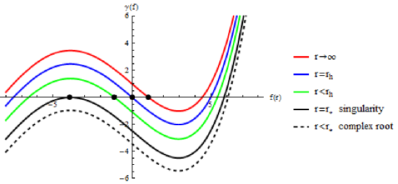
Figure 2: $\gamma(f)$ versus $f(r)$ for different $r$. Black dots show the value of $f(r)$ for a black hole solution at different $r$. Note how $f(r)$ increases from a negative value at $r=r_{\ast}$ to a positive value as $r\to\infty$, and it is complex for $r<r_{\ast}$.

In order to analyze the extrema of $\gamma=\gamma(x)$, we may study the roots of $\gamma^{\prime}(\tilde{x})=0$,

$$\tilde{x}^{3}+\frac{3\mu}{4\nu}\tilde{x}^{2}-\frac{1}{4\nu}=0.$$ (31)

The Vieta’s formulas $\tilde{x}_{1}\tilde{x}_{2}\tilde{x}_{3}=(-1)^{3}(-1/4\nu)$ and $\tilde{x}_{1}\tilde{x}_{2}+\tilde{x}_{1}\tilde{x}_{3}+\tilde{x}_{2}\tilde{x}_{3}=0$ imply

$$\frac{1}{\tilde{x}_{1}}+\frac{1}{\tilde{x}_{2}}+\frac{1}{\tilde{x}_{3}}=0.$$ (32)

Moreover, a cubic equation like $\gamma^{\prime}(\tilde{x})=0$ has three real roots or one real and two complex roots. The former leads to the possibility of the existence of two negative roots and one positive or vice versa. The later shows the real root may be either positive or negative. On the other hand, The sign of product of roots depends on sign of $\nu$. By using these hints, one finds that for $\nu>0$ there are one real positive and two complex roots or one positive and two negative real roots. Also for $\nu<0,~{}$there are one real negative and two complex roots or one negative and two positive real roots. In addition, one may consider the condition of the existence of complex roots for our cubic equation by investigating the sign of the discriminant function $\mathcal{D}=4\nu^{4}-\mu^{3}\nu^{2}.$ When $\mathcal{D}>0$ there are one real and two complex roots and for $\mathcal{D}<0~{}$all the roots are real. We will ignore special cases where $\mathcal{D}=0$ here (see Myers1 for useful information on cubic equation). By using these facts, we may easily study the conditions of existence of black hole as follows (see table 1).

Consider case (a) of table 1, which admits four real roots for $\gamma=\gamma(x)$ corresponding to two AdS and two dS solutions. This condition shows the existence of three extrema as one may see in Fig. 3. A positive extremum occur between the two AdS and a negative must locate between the two dS solutions. Third extremum could be either negative or positive. However, as we mentioned above the sign of product of the roots is determined by the sign of $\nu$. So, for region (a) ($\nu>0$) third extremum must be negative and therefore there is a black hole solution, which is $f_{3}$. Now let us examine the case (b) of table 1 with one negative and three positive real roots corresponding to one dS and three AdS solutions (see Fig. 3). In these cases, there are three extrema. Two of them occur between the three AdS solutions. But the other one must be between the smallest AdS solution and the dS one. On the other hand, by considering Eq. (32), this extremum must be negative. So, there is a black hole solution in this case. It is clear that in this situation the smallest AdS solution could correspond to asymptotic value of an AdS planar black hole. In this region $f_{2}$ describes the black hole solution. In case (c) of the table, there is no AdS solution as it is seen in Fig. 3. Next we consider the regions (d) and (e) where there are two AdS solutions and no dS one. In this cases there is a positive extremum between the two AdS solutions as one may see in Fig. 3. Since for $\nu>0$ there is no other positive extremum, a black hole solution exists. One may see the above consideration in Fig. 3. In the region (f), there are an AdS and a dS solution. An extremum occurs between the dS and the AdS solutions which may relate to either a black hole or a naked singularity depending on the sign of this extremum. For $\mathcal{D}<0$ there is only one real root for cubic equation which shows the existence of only one extremum (see Fig. 3). So for $\nu<0$, one may find that this extremum must locate in the negative region and therefore, a black hole could exist. However for $\mathcal{D}>0$, there are three real roots for cubic equation and so three extrema which two of them must be positive. It is possible that one of them locates between zero and the ghost free AdS. So, this condition excludes black hole solution. But, one may consider the possibility of existence of black hole for $\mathcal{D}>0$ when the two positive roots are greater than the ghost free AdS solution. One may analyze this situation numerically. The region of the parameter space for which a black hole may exist has been shown in Fig. 4. Up to now we study the possibility of existence of any extremum for $x\in(0,f_{\infty})$. This corresponds to the situation where there is a real metric function $f(r)$ which admits a horizon at $r_{h}$ and increases monotonously from $0$ to $f_{\infty}$.

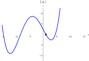
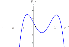
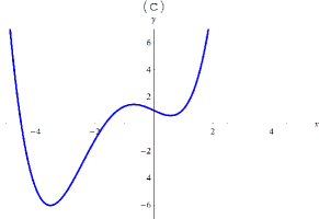
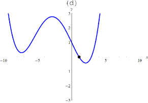
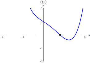
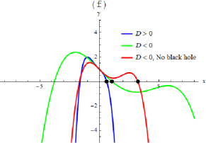
Figure 3: Behavior of $\gamma$ as the function of $x$. Black dot in each figure indicates the ghost free AdS vacuum.

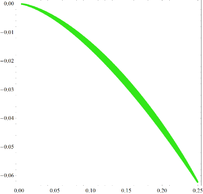
Figure 4: This plot displays a part of region (f) for which $\mathcal{D}<0$ and a black hole solution exists.

	$\Delta$	$\delta$	Real Roots	$\nu$	$\mu$	dS	Ghost Free AdS	ghosty AdS	AdS Black Hole
a	+	+	4	+	+	2	1	1	$f_{3}$
b	+	+	4	-	+	1	2	1	$f_{2}$
c	-	$\pm$	2	+	$\mu>0,~{}G>0$	2	0	0	-
d	-	$\pm$	2	+	$\mu>0,~{}G<0$	0	1	1	$f_{3}$
e	-	$\pm$	2	+	-	0	1	1	$f_{3}$
f	-	$\pm$	2	-	$\pm$	1	1	0	$\mathcal{D}>0$, $f_{2}$ $\mathcal{D}<0$, $f_{2}$ or no black hole.
g	+	-	0	No Real Roots

Table 1: Table of various vacua and black hole solutions.

Before ending this section, we give a comment on the special case $\lambda=\mu=0$ for which $H$ vanishes. So one may study it with more care. In this case the discriminant functions $\Delta,~{}\delta$, $G$ and $D$ reduce to

$$\Delta = -\frac{{27}}{{{\nu^{4}}}}(27+256\nu),\quad\delta=-\frac{64}{\nu}$$

$$G = -\frac{8}{\nu},\quad\mathcal{D}=4\nu^{4}>0.$$

Thus, for $\nu>27/256$, $\Delta$ is positive and so there is no real root. However, for $\nu<27/256$  there exist two real roots Math which may be studied as follows. Since $\mathcal{D}>0$, there is only one extremum for $\gamma(x)$ which is positive for $\nu<0$ and negative for $\nu>0$ due to the fact that $\tilde{x}_{1}\tilde{x}_{2}\tilde{x}_{3}=(-1/4\nu)$. Now, by using asymptotic behaviour of $\gamma(x)\approx\nu x^{4}$ for $x\rightarrow\infty$ and $\gamma(0)=1$, it is easy to see that for $\nu>0$ there is a ghost free AdS and a ghosty AdS solution. However, the case $\nu<0$ admits a ghost free AdS and a dS solution. Thus, for $\nu<27/256$ a ghost free AdS black hole solution always exists. This solution is given by $f_{3}$ for $\nu>0$ and $f_{2}$ for $\nu<0$.

Up to now we have considered the cases with $\lambda=0$ and found the regions of parameter space where AdS black holes exist. For investigation of the general cases in the presence of Gauss-Bonnet term, one should use the same argument as the above considerations. We will not study the general case in details, but we consider some special examples which will be used in the following sections. As a first example, we consider a special point in parameter space in a region which does not admit black hole for $\lambda=0$. A point with this property occurs for example at $\mu=0.4$ and $\nu=-0.05$. Figure 5 shows that a black hole solution exists only for $\lambda<-0.257$. As a second example, consider the point ($\lambda=0$, $\mu=0.06$, $\nu=0.02$) in parameter space which is in a region that admits black hole solution. As one may see from Fig. 5, a black hole exists for $\mu=0.06$, $\nu=0.02$ in the presence of Gauss-Bonnet term provided $\lambda<0.088$.

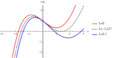
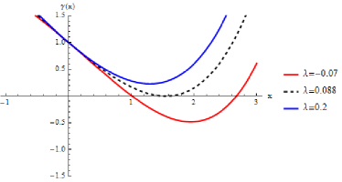
Figure 5: Left figure: $\gamma(x)$ versus $x$ for $\mu=0.4,\nu=-0.05$ and various $\lambda$. Black hole solutions exist for $\lambda<-0.257$. Right figure: $\gamma(x)$ versus $x$ for $\mu=0.06,\nu=0.02$ and various $\lambda$. Black hole solutions exist for $\lambda<0.088$.

7 Weyl Anomaly and Central Charges

In this section, we use the AdS/CFT duality for finding the central charges of CFT dual to quartic quasi-topological gravity. Indeed, when a CFT is placed on a curved background the trace of energy-momentum tensor, which is related to the central charges of CFT, is non-zero and one encounters a Weyl anomaly (for a historical review see Duff ). By finding these central charges, we want to develop the dictionary relating the couplings in five-dimensional quasi-topological gravity to the parameters which characterizes its dual four-dimensional CFT. For a CFT in four dimensions, the trace anomaly relation may be written as

$$\langle T_{a}^{a}\rangle=\frac{c}{16\pi^{2}}I_{4}-\frac{a}{16\pi^{2}}E_{4},$$ (33)

where

$$I_{4}=R_{ijkl}R^{ijkl}-2R_{ij}R^{ij}+\frac{1}{3}R^{2}\ \ \text{and}\ \ \ \ \ E_{4}=R_{ijkl}R^{ijkl}-4R_{ij}R^{ij}+R^{2}$$ (34)

are the square of Weyl tensor and Euler density in four dimensions, respectively.

In order to compute $a$ and $c$, there is a standard approach in the context of AdS/CFT correspondence CentCharg1 . One can start with gravity action and uses the Fefferman-Graham expansion of the metric

$$ds^{2} = \frac{L_{eff}^{2}}{4\rho^{2}}d\rho^{2}+\frac{\bar{g}_{ij}}{\rho}dx^{i}dx^{j},$$ (35)

$$\bar{g}_{ij} = \bar{g}_{(0)ij}+\rho\bar{g}_{(1)ij}+\rho^{2}\bar{g}_{(2)_{ij}}+...~{},$$ (36)

where $\bar{g}_{(0)ij}$ denotes the boundary metric. The holographic approach instructs us to plug this expansion into the action and use the field equations to eliminate $\bar{g}_{(2)ij}$. The resultant action will be in terms of $\bar{g}_{(0)ij\text{ }}$ and$~{}\bar{g}_{(1)ij}$, while the latter can be found in term of $\bar{g}_{(0)ij\text{ }}$ through the use of field equations. Then, in order to find the Weyl anomaly, one needs only those terms which produce a log divergence, that is

$$I\backsim\frac{1}{2}\ln\epsilon~{}\int d^{4}x~{}\sqrt{\bar{g}_{(0)}}\langle T_{a}^{a}\rangle,$$ (37)

where $\epsilon~{}$is a cut off limit.

However, doing such messy calculations for higher order gravity are cumbersome. So we use the nice trick used in Ref. Sinha for calculating the central charges . We take the boundary $\bar{g}_{ij}$ as

$$d\bar{s}^{2}=u[1+\alpha\rho](-R^{2}dt^{2}+\frac{dR^{2}}{4R^{2}})+v[1+\beta\rho](d\theta^{2}+\sin^{2}\theta d\phi^{2}).$$ (38)

Thus, the bulk metric is

$$ds^{2}=\frac{L_{eff}^{2}}{4\rho^{2}}d\rho^{2}+\frac{1}{\rho}\left\{u(1+\alpha\rho)\left(-R^{2}dt^{2}+\frac{dR^{2}}{4R^{2}}\right)+v(1+\beta\rho)(d\theta^{2}+\sin^{2}\theta d\phi^{2})\right\}.$$ (39)

We substitute the metric (39)  into the action and extract the term proportional to $1/\rho$, which leads to logarithmic divergence. Using the field equations for the metric (35), and denoting the logarithmic term as $L_{\ln}$, one finds

$$\frac{\partial}{\partial\alpha}L_{\ln}=0;\ \ \ \ \ \ \ \ \ \ \ \ \ \ \ \ \frac{\partial}{\partial\beta}L_{\ln}=0,$$ (40)

which gives $\alpha$ and $\beta$ in terms of other parameters. The expressions $E_{4}$ and $I_{4}$ for $\bar{g}_{0(ij)}$ background can be calculated as

$$E_{4}=\frac{-8}{u~{}v},\ \ \ \ \ \ \ \ \ \ \ \ \ \ \ \ \ I_{4}=\frac{4(u-v)^{3}}{3u^{2}v^{2}}.$$ (41)

Now, it is straightforward to show that central charges can be obtained by using the following equations

$$c = \left(\lim_{v\longrightarrow\infty}\frac{24\pi^{2}L_{\ln}}{\sqrt{\bar{g}_{(0)}}}\right)_{u=1},$$

$$a = \left(\lim_{v\longrightarrow 1}\frac{4\pi^{2}L_{\ln}}{\sqrt{\bar{g}_{(0)}}}\right)_{u=1}.$$

For quartic quasi-topological gravity such calculations lead to

$$c = \frac{\pi^{2}L^{3}}{f_{\infty}^{\frac{3}{2}}l_{p}^{3}}(1-2\lambda f_{\infty}-3\mu f_{\infty}^{2}-4\nu f_{\infty}^{3}),$$

$$a = \frac{\pi^{2}L^{3}}{f_{\infty}^{\frac{3}{2}}l_{p}^{3}}(1-6\lambda f_{\infty}+9\mu f_{\infty}^{2}+4\nu f_{\infty}^{3}),$$

which reduce to the central charges of cubic quasi-topological Myers2 for $\nu=0$. It is worthwhile to mention that the central charge $c$ is proportional to the two-points correlation function of energy-momentum tensor, and therefore in order to have unitary CFT, $c$ should be positive. This result is in agreement with the condition (26) as one may expect. Indeed both of them arise from the graviton propagation in AdS background analysis, and therefore they should impose the same constraint on the parameters of gravity theory.

8 Causality Constraint in Tensor Channel

In this section, we perform the causality study of CFT in 4 dimensions duals to the 5-dimensional quartic quasi-topological gravity. It is known that the existence of a black hole in the bulk spacetime breaks Lorentz invariant of dual CFT, and therefore one should consider the possibility of propagation of superluminal modes in the CFT and violation of causality. In order to avoid causality violation, one may constrain the gravitational coupling. Actually, this kind of analysis has been performed for the first time in Gauss-Bonnet gravity in Ref. Liu , and then extended to other higher order theories of gravity de Bore1 ; Edelstein1 ; de Bore2 ; GBd ; Buchel . Here we only study tensor channels analysis, and we leave the other channels analysis for future.

Naturally, the existence of higher curvature terms in a theory of gravity leads to new coupling parameters and therefore new causality constraints. However, surprisingly, cubic quasi-topological gravity does not show any new causality constraints Myers2 . So the question is: does quartic quasi-topological gravity has the same trivial result? Indeed, one of our main motivation for studying quartic quasi-topological gravity is these kinds of investigations. As we will see in this section, considering only quartic term without the cubic term leads to a trivial result, just like in the cubic quasi-topological gravity. However, if one considers both cubic and quartic terms, then a non-trivial result will be appeared. Here we study the causality in the tensor channel by following the procedure of Ref. Myers2 , closely.

Consider a black hole background such as (14), which is deformed by a tensor perturbation to

$$ds^{2}=\frac{r_{h}^{2}}{L^{2}\rho}\left(-f(\rho)dt^{2}+d\overrightarrow{x}^{2}+2\phi(\rho)e^{i(qx_{3}-\omega t)}dx_{1}dx_{2}\right)+\frac{L^{2}}{4\rho^{2}}\frac{d\rho^{2}}{f(\rho)},$$ (42)

where we define $\rho=r_{h}^{2}/r^{2}$ in Eq. (17). The linearized equation of perturbation $\phi(\rho)$ may be written as

$$\nu\partial_{\rho}[C_{(4)}(\rho)\phi^{(3)}(\rho)+C_{(4)}^{\prime}(\rho)\phi^{{}^{\prime\prime}}(\rho)]+\partial_{\rho}[C_{(2)}(\rho,q^{2},\omega^{2})\phi^{{}^{\prime}}(\rho)]+C_{(0)}(\rho,q^{2},\omega^{2})\phi(\rho)=0,$$ (43)

where $\phi^{(i)}$ denotes the $i$th-order derivative of $\phi$ with respect to $\rho$, $C_{(4)}$ is

$$C_{4}(\rho)=\frac{6464}{73}\rho^{3}f^{2}r_{h}^{2}(\rho^{2}f^{\prime\prime 2}-\frac{22}{101}\rho f^{\prime}f^{\prime\prime}+\frac{3}{4}f^{\prime 2}),$$ (44)

and $C_{(0)}$ and $C_{(2)}$ are given in the Appendix. One may note that the presence of third and fourth-order derivatives of  $\phi$ with respect to $\rho$ is a feature of quartic quasi-topological gravity which is different from the cubic quasi-topological gravity. We may emphasize that this perturbation is around a black hole solution and for perturbation around the AdS solution ($f(\rho)=const.$), $C_{(4)}$ vanishes as one may see in Eq. (44). Indeed, in the cubic theory the graviton wave equation around a black hole background is second order in the radial derivative of $\phi(\rho)$ and therefore it is convenient to convert it to a Schrodinger like form and study the graviton wave function. Although in quartic quasi-topological gravity the graviton wave equation (43) is not second order, but for our purpose it is sufficient to work at large momentum and frequency limit of Eq. (43). In fact, the dispersion relation for $\omega$ and $q$ determines the front velocity of the signals as $v_{front}=\lim_{q\rightarrow\infty}Re(\omega)/q$. At this limit, we focus on the last term $C_{(0)}(\rho,q^{2},\omega^{2})$, which is the dominant term.

Let’s review the case of Gauss-Bonnet gravity ($\mu=0=\nu$), for which the dominant term reduces to

$$0 = C_{(0)}(\rho,q^{2},\omega^{2})=219r_{h}^{2}L^{4}f_{\infty}f(\rho)(1-2\lambda f(\rho)+2\rho f^{\prime}(\rho))\omega^{2}$$

$$-219r_{h}^{2}L^{4}\rho f(\rho)^{2}(1-2\lambda f(\rho)+2\lambda\rho f^{\prime}(\rho)-4\rho^{2}\lambda f^{\prime\prime}(\rho))q^{2},$$

where $f_{\infty}=f(\rho=0)$. By using the near boundary expansion ($r\rightarrow\infty$ or $\rho\rightarrow 0$) of $f(\rho)$ in Gauss-Bonnet gravity, one obtains

$$\frac{\omega^{2}}{q^{2}}=1-\frac{1-10\lambda f_{\infty}}{(1-2\lambda f_{\infty})^{2}f_{\infty}}\rho^{2}+O(\rho^{4}),$$ (45)

which shows that the superluminal signals will be avoided, provided $1-10\lambda f_{\infty}\geq 0$.

In the quartic quasi-topological gravity, the constant $C_{(0)}(\rho,q^{2},\omega^{2})$ contains terms proportional to $q^{2}\omega^{2}$, $\omega^{4}$ and $q^{4}$ (see Appendix), while in the cubic quasi-topological gravity there is no $\omega^{4}$-term. By taking $\omega^{2}=\alpha^{2}q^{2}$ and solving for $\alpha^{2}$, one obtains

$$\lim_{q\rightarrow\infty}\alpha^{2}=\frac{f}{f_{\infty}}\frac{[1314\rho f^{\prime\prime}+657f^{\prime}]\mu-[6624\rho^{3}f^{\prime\prime 2}-24\rho(73f-74\rho f^{\prime})f^{\prime\prime}+168\rho f^{\prime}{}^{2}-876ff^{\prime}]\nu}{[1314\rho f^{\prime\prime}+657f^{\prime}]\mu-[14400\rho^{3}f^{\prime\prime 2}-24\rho(73f-\frac{512}{3}\rho f^{\prime})f^{\prime\prime}+5708\rho f^{\prime 2}-876ff^{\prime}]\nu}.$$ (46)

It is worth noting that although the above equation does not depend on $\lambda$ explicitly, but it depends on $\lambda$ because of the dependence of $f(r)$ on $\lambda$. For cubic quasi-topological gravity ($\nu=0$), this equation reduces to $f(\rho)/f_{\infty}$, which is the same as that of Einstein gravity. But, in quartic quasi-topological gravity, Eq. (46) reduces to

$$\lim_{q\rightarrow\infty}\alpha^{2}=1-\frac{11300f_{\infty}\nu+657\mu}{219(1-2\lambda f_{\infty}-3\mu f_{\infty}^{2}-4\nu f_{\infty}^{3})(4f_{\infty}\nu+3\mu)f_{\infty}}\rho^{2}+O(\rho^{3}),$$

where we have used the near boundary expansion, $f(\rho)=f_{\infty}-(1-2\lambda f_{\infty}-3\mu f_{\infty}^{2}-4\nu f_{\infty}^{3})^{-1}\rho^{2}+O(\rho^{3})$. Since $(1-2\lambda f_{\infty}-3\mu f_{\infty}^{2}-4\nu f_{\infty}^{3})>0$, the following inequality

$$\frac{11300f_{\infty}\nu+657\mu}{(4f_{\infty}\nu+3\mu)f_{\infty}}\geq 0,$$ (47)

guarantees the near boundary causality in the tensor channel. It is worth to note that in the absence of either of the two quasi-topological terms ($\mu=0$ or $\nu=0$), no constraint is imposed on the coupling constants because of causality.

To determine the region where causality is violated, one need to consider which roots of $\gamma(f_{\infty})=0$ corresponds to the black hole solution. Indeed, for each value of  ($\lambda,\mu,\nu$) that admit AdS planar black hole, we check which root of the quartic equation corresponds to black hole. Then we take $f_{\infty}$ associate to the black hole root and we plot the region where causality violates in the tensor channel for the special case $\lambda=0$ (Fig.6). Numerical calculations show that the sensitivity of casual region with respect to variation of $\lambda$ is not considerable. This is due to the fact that Eq. (47) does not depend on $\lambda$ explicitly and $f_{\infty}$ is of order one.

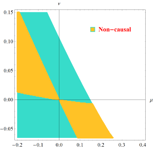
Figure 6: The orange and green regions show the non-casual and casual regions, respectively in the tensor channel in the absence of Gauss-Bonnet term.

9 Holographic hydrodynamics

In order to study the effects of causality on the viscosity/entropy ratio, we will use the calculations inspired by AdS/CFT correspondence Liu ; Kss . Such calculations have been performed for cubic and quartic quasi-topological gravity in Myers2 ; Dehghani1 . Here, for completeness, we give a brief review of the interesting pole method Paulos which has been used in Dehghani1 in order to obtain shear viscosity for a planar metric which admits black hole solution. Following the method of Refs. Myers2 ; Paulos and employing the transformation $u=1-r_{h}^{2}/r^{2}$ to map horizon-boundary region $r\in(r_{h},\infty)$ to $u\in(0,1)$, the metric (14) becomes

$$ds^{2}=\frac{r_{h}^{2}}{L^{2}(1-u)}(-\frac{f(u)}{f_{\infty}}dt^{2}+dx^{2}+dy^{2}+dz^{2})+\frac{L^{2}}{4f(u)}\frac{du^{2}}{(1-u)^{2}}.$$ (48)

We expand $f(u)$ around the simple zero at the horizon $u=0$

$$f(u)=2u+(4\lambda-1)u^{2}+4(2\mu+\lambda(4\lambda-1))u^{3}+O(u^{4}).$$

Now we perturb the metric by the transformation $dx\rightarrow dx+\varepsilon e^{-i\omega t}dy$, where $\varepsilon~{}$is an infinitesimal positive parameter and evaluate the Lagrangian $\mathcal{\tilde{L}}\equiv\sqrt{-g}\mathcal{L}_{g}$ on the perturbed metric. The off-shell perturbation produces a pole at $u=0$ which the residue of this pole gives us the shear viscosity

$$\eta=8\pi T\lim_{\omega,\rightarrow 0}\frac{\text{Res}_{u=0}\mathcal{L}}{\omega^{2}\varepsilon^{2}}.$$ (49)

In Eq. (49) $T$ is the temperature of black hole given in Eq. (20) and Res${}_{u=0}\mathcal{\tilde{L}~{}}$ stands for the residue of the pole at $u=0$. One obtains the viscosity/entropy ratio as

$$\frac{\eta}{s} = \frac{1}{4\pi}[1-4\lambda-36\mu(9-64\lambda+128\lambda^{2}+48\mu)$$ (50)

$$-\frac{96}{73}\nu(1491+6240\mu-10752\mu\lambda$$

$$-10800\lambda+28864\lambda^{2}-25088\lambda^{3})],$$

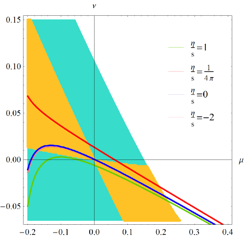
Figure 7: Contours of constant $\frac{\eta}{s}$

which shows that, in contrast to Lovelock gravity, the cubic and quartic terms have contributions in the $\eta/s$ shearlovelock . For $\lambda=0$ this ratio reduce to

$$\frac{\eta}{s}=\frac{1}{4\pi}[1-36\mu(9+48\mu)-\frac{96}{73}\nu(1491+6240\mu)].$$

In Fig. 7 we plot the contours $\eta/s=const$ on the ($\mu,\nu)$ plane. From this plot, it is clear that the near boundary causality constraint in the tensor channel is not strong enough to preserve a positive bound on $\eta/s$. Of course, this fact is a common feature of higher order curvature gravities such as third order Lovelock or cubic quasi-topological gravities Edelstein1 ; de Bore2 . However in the case of cubic quasi-topological gravity, the positive energy constraint restores a lower positive bound on $\eta/s$ which excludes the negative value for $\eta/s$ Myers2 . Thus, we expect that the positive energy constraints in different channels may restore a positive bound on $\eta/s$ in our case too, but we leave it for future.

Another possibility is the consideration of interior geometry causality constraint. We studied the tensor channel causality in the near boundary by using the asymptotic expansion of the metric function and found some constraints on the coupling constants. However, as mentioned in EdelsteinPaulos , the causality may be violated in the interior geometry in Lovelock gravity. So, studying the causality in the bulk may imply a stronger constraint on the parameter space and perhaps restores a positive bound on $\eta/s$. General studies of this issue is cumbersome, but to understand the probable effects of bulk causality on the negativity of $\eta/s$ we take $\mu=.06$, $\nu=.02$ and $\lambda=-0.07,0,0.07$. As one can see in Fig. 5, for these choices a black hole solution exists. In Fig.8, we plot $\alpha^{2}$ by substituting the metric function of the black hole solution in Eq. (46). This plot shows that $0\leq\alpha^{2}\leq 1$. Also, these values lead to negative viscosity. Thus, it seems that this constraint has no chance to keep $\eta/s$ to be positive. However, there are some restrictions about our result. Indeed, the existence of higher derivative terms in the field equation of graviton on the black hole background does not allow us to write the wave equation in the neat Schrodinger form and analyze the potential. So, perhaps one needs to treat the effective dispersion relation $\alpha$ with more care. Also, it is worth to mention that our investigation is done for 5-dimensional spacetime and the bulk causality constraint is sensitive to the dimension of the spacetime.

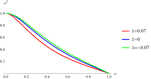
Figure 8: Plot of $\alpha^{2}$ in term of $\rho$ for $\mu=.06$ and $\nu=.02$. The plot shows the $\alpha^{2}$ is positve and less than one for every where between horizon and boundary.

In addition, there is another source of constraints for the gravitational coupling coming from the instabilities of the plasma in the dual theory GBd . Indeed, this issue occurs when the local speed of graviton becomes imaginary $\alpha^{2}<0$. This constraint, implies a lower positive bound on $\eta/s$ in Lovelock theory EdelsteinPaulos , but as we have seen above this cannot implies any positive lower bound on $\eta/s$ in 5-dimensional quasi-topological gravity. But, as we have mentioned above this investigation is sensitive to the dimension of the spacetime.

10 Concluding Remarks

In this paper, we considered quartic quasi-topological gravity in the presence of negative cosmological constant in five dimensions. We varied the action with respect to the metric $g^{ab}$ and found the general tensorial form of field equation for quartic quasi-topological gravity with cubic and quartic terms in Riemann tensor. In general, this field equation includes forth-order derivatives. But for the special choices of coefficients, $c_{i}$’s, given in Eq. (3) and spherically symmetric spacetimes, the field equation is second-order. Moreover, we showed that a linearized perturbation around an AdS spacetime reduces to a second-order wave equation for graviton which matches to Einstein’s gravity up to an overall factor. By considering the sign of this overall factor, we constrained the coupling parameters in order to have ghost free AdS solutions. In the case of quasi-topological gravity (as like as Lovelock gravity), the field equation for spherically symmetric ansatz leads to a polynomial equation (quartic equation for quartic quasi-topological gravity). For simplicity, we analyzed the quartic equation in the absence of Gauss-Bonnet term and found the region of parameter space where ghost free AdS solutions exist. In addition, we determined the region of parameter space where the existence of planar AdS black hole is possible. As one may expect, there are some regions where ghost free AdS solution exists but there is no black hole. These cases occur when there are double roots solutions for the quartic equation. In these cases, by studying the Kretchman curvature scalar, we explicitly showed that the spacetime involves a naked singularity. However, it is interesting to generalize these discussions for curved boundary and higher-dimensional spacetime Lovebes . We, also, considered the general case in the presence of Gauss-Bonnet term for a few special values of $\mu$ and $\nu$.

In the context of AdS/CFT, we found the central charges of CFT₄ dual to the quartic quasi-topological gravity. We found that the unitary of the CFT₄, which implies the positivity of central charge and relates to the energy-momentum tensor two-point function, is the same as the stability constraint which comes from the study of perturbation around AdS₅. We also studied tensor-channel perturbation around a black hole background to find the effects of quasi-topological gravity on the causality violation. We obtained the equation for linearized perturbation around a black hole solution and found that it includes forth-order derivatives. However, in the absence of the quartic term this equation reduces to a second-order one. Moreover, in contrast to cubic quasi-topological and (Weyl)² gravities which do not show any causality violation, we showed that the existence of cubic and quartic terms together provide the possibility of causality violation. So in order to survive causality, one needs to imply some constraints on the region of parameter space where black holes may exist. We also considered causality constraints in the tensor channel on the viscosity/entropy ratio and found that this constraint is not strong enough to imply any positive bound on the viscosity/entropy ratio. We also studied the possibility of violation of tensor channel causality and instabilities in the interior geometry in five dimensions for some special cases. But, the positivity of $\alpha^{2}$ does not imply any positive bound on $\eta/s$. Although this is in contrast to Lovelock gravity in seven dimensions, but one should note that $\alpha^{2}$ is sensitive to the dimensions of the spacetime. Also, because of the existence of higher order derivatives, perhaps more careful study of quasi normal modes is necessary.

It is known that for supersymmetric theory the causality and positive energy conditions are related Hofman . Here, we address the interesting study in relation between causality and positive energy constraints for a non-supersymmetric theory like quasi-topological gravity Myers2 ; Hofman . Indeed, this was one of the essential motivations for studying quasi-topological gravity in a five-dimensional spacetime. But this comparison is not possible in cubic gravity frame work, since the causality does not imply any constraint Myers2 . However in quartic quasi-topological gravity, as we have discussed above, the causality in the tensor channel creates a new constraint but it is not strong enough to imply any bound on the viscosity/entropy ratio. Thus, one may consider the possibility of causality violation in other channels GBd or positive energy constraint for quartic quasi-topological gravity in order to survive this ratio. In addition, the full study of perturbation around a black hole solution in the various channels GBd ; othercha and finding the quasi-normal modes in order to find the possibility of causality violation or instability are interesting. They may imply a positive bound on $\eta/s$ as in the case of Lovelock theory GBd ; EdelsteinPaulos . Besides, as it is mentioned in EnerUnit the positivity of energy flux is equivalent to the absence of ghost in the finite temperature conformal field theory. So, it is worthwhile to study this property directly in the quasi-topological gravity. Also by using the central charges calculated in this paper, one may study the effects of quartic quasi-topological term on the holographic c-theorem Ctheo and entanglement entropyRyu . We leave these interesting topics for future works.

Appendix A The coefficients $C_{(0)}$ and $C_{(2)}$

The constant $C_{(0)}(\rho,q^{2},q^{4},\omega^{2},\omega^{4})=-\tilde{C}_{(0)}/(438r^{3}f^{2}r_{h}^{2}L^{4})$ in Eq. (43) for the case of quartic quasi-topological gravity is

$$\tilde{C}_{(0)} = 219\,{L}^{4}{f_{\infty}}r_{h}^{2}\rho f[1-2\lambda(f+\rho{f^{\prime}}\,)]{\omega}^{2}+219\,{L}^{4}r_{h}^{2}\rho{f}^{2}[-1+2\,f\lambda+4\,{\rho}^{2}f^{\prime\prime}\,\lambda-2\,\rho f^{\prime}\,\lambda]{q}^{2}$$

$$-657\,{L}^{4}f_{\infty}{r}_{h}^{2}\,\rho f[12\,{\rho}^{4}f^{(4)}f+6\,{\rho}^{3}\left(\rho f^{\prime}+8\,f\right)f^{(3)}+6\,{\rho}^{4}f^{\prime\prime 2}+\left(18\,{\rho}^{3}f^{\prime}+27\,{\rho}^{2}f\right)f^{\prime\prime}$$

$$+{f}^{2}+3\,{\rho}^{2}f^{\prime 2}-2\,\rho f^{\prime}\,f]\mu\,\omega^{2}-12\,{L}^{4}f_{\infty}{r}_{h}^{2}\rho\,\{\left(944\,{\rho}^{6}f^{\prime\prime}\,-1064\,{\rho}^{5}f^{\prime}\,+876\,{\rho}^{4}{f}\right){f}^{2}f^{(4)}$$

$$+944\,{\rho}^{6}f^{(3)2}{f}^{2}+((-1952\,{\rho}^{6}f^{\prime}\,+4872\,{\rho}^{5}{f})f^{\prime\prime}+3504\,{\rho}^{3}{f}^{2}-4042\,{\rho}^{4}f^{\prime}\,{f}$$

$$+[(-1952\,{\rho}^{6}f^{\prime}\,+4872\,{\rho}^{5}{f})f^{\prime\prime}+3504\,{\rho}^{3}{f}^{2}-4042\,{\rho}^{4}f^{\prime}\,{f}-268\,{\rho}^{5}f^{\prime 2}]ff^{(3)}$$

$$-976\,{\rho}^{6}f^{\prime\prime 3}f+\left(808\,{\rho}^{6}f^{\prime 2}+1514\,{\rho}^{4}{f}^{2}-4440\,{\rho}^{5}f^{\prime}\,f\right)f^{\prime\prime 2}$$

$$+\left(1971\,{f}^{3}{\rho}^{2}-1234\,{f}^{2}{\rho}^{3}f^{\prime}-176\,{\rho}^{5}f^{\prime 3}-3426\,{\rho}^{4}ff^{\prime 2}\right)f^{\prime\prime}$$

$$+606\,{\rho}^{4}f^{\prime 4}-219\,{f}^{3}f^{\prime}\,\rho+73\,{f}^{4}-1821\,{\rho}^{3}f^{\prime 3}f+452\,{f}^{2}f^{\prime 2}{\rho}^{2}\}\nu\omega^{2}$$

$$-657\,\,{L}^{4}{\ }r_{h}^{2}\rho{f}^{2}[12{\rho}^{4}f\ f^{(4)}+12{\rho}^{3}\left(\rho f^{\prime}+4\,f\right)f^{(3)}+(23\,{\rho}^{2}f+24\,{\rho}^{3}f^{\prime})f^{\prime\prime}-\,(\rho f^{\prime}-f)^{2}]\mu{q}^{2}$$

$$+12\,{L}^{4}r_{h}^{2}\rho{f}^{2}[\left(1368\,{\rho}^{5}f^{\prime}\,f-592\,{\rho}^{6}f^{\prime\prime}\,f-876\,{\rho}^{4}{f}^{2}\right)f^{(4)}-592\,{\rho}^{6}f^{(3)2}f$$

$$+((-592\,{\rho}^{6}f^{\prime}+1280\,{\rho}^{5}f)f^{\prime\prime}+5428\,{\rho}^{4}f^{\prime}\,f-3504\,{f}^{2}{\rho}^{3}+1368\,{\rho}^{5}f^{\prime 2})f^{(3)}$$

$$+\left(1140\,{\rho}^{5}f^{\prime}+6496\,{\rho}^{4}f\right)f^{\prime\prime 2}+(1334\,ff^{\prime}\,{\rho}^{3}+3076\,\rho^{4}f^{\prime 2}-1533\,{f}^{2}{\rho}^{2})f^{\prime\prime}$$

$$+73\,{f}^{3}-657\,{\rho}^{3}f^{\prime 3}-219\,f^{2}f^{\prime}\,\rho-219\,ff^{\prime 2}\rho^{2}]\nu{q}^{2}$$

$$-6\,{L}^{8}f_{\infty}^{2}{\rho}^{4}(-88\,\rho{\ }f^{\prime}\,f^{\prime\prime}+303\,f^{\prime 2}+404\,{\rho}^{2}f^{\prime\prime 2})\nu\,\omega^{4}+657\,{L}^{8}{\rho}^{3}{f}^{2}\left(f^{\prime}+2\,\rho f^{\prime\prime}\right)\mu{q}^{4}$$

$$-3\,{L}^{8}{\rho}^{3}{f}^{2}\left(2208\,{\rho}^{3}f^{\prime\prime 2}-8\,\rho\left(-74\,\rho f^{\prime}+73\,f\right)f^{\prime\prime}+56\,\rho f^{\prime 2}-292\,f^{\prime}\,f\right)\nu{q}^{4}$$

$$+{L}^{8}f_{\infty}{\rho}^{3}f\,(-657\,f^{\prime}-1314\,\rho~{}f^{\prime\prime})\mu{q}^{2}\omega^{2}$$

$$+{L}^{8}f_{\infty}\,{\rho}^{3}f(14400\,{\rho}^{3}f^{\prime\prime 2}-8\,\left(-512\,\rho f^{\prime}+219\,f\right)\rho f^{\prime\prime}+5708\,\rho f^{\prime 2}-876\,f^{\prime}\,f)\nu{q}^{2}\omega^{2}.$$

which contains terms proportional to $q^{2}\omega^{2}$, $\omega^{4}$ and $q^{4}$. Also, $C_{(2)}$ is

$$C_{(2)} = [6\,f(\rho)\rho\,(2\,\rho\,{f^{\prime\prime}}+{f^{\prime}})\mu+{\frac{8}{219}}\,\rho\,f(438\,\rho\,{f^{\prime\prime}}\,f+219\,{f^{\prime}}\,f$$

$$-1024\,{\rho}^{2}{f^{\prime\prime}}\,{f^{\prime}}-3600\,{\rho}^{3}{{f^{\prime\prime}}}^{2}-1427\,\rho\,{{f^{\prime}}}^{2})\nu]{q}^{2}$$

$$+{\frac{8}{73}}\,{\rho}^{2}{f_{\infty}}\,[-88\,\rho{f^{\prime\prime}}\,{f^{\prime}}+404\,{\rho}^{2}{{f^{\prime\prime}}}^{2}+303\,{{f^{\prime}}}^{2}]\nu\,{\omega}^{2}$$

$$+6\,{\frac{f{r}_{h}^{2}\mu}{\rho\,{L}^{4}}}[6\,{f^{\prime}}\,{\rho}^{4}{f^{(3)}}+18\,{f^{\prime}}\,{\rho}^{3}{f^{\prime\prime}}+6\,{\rho}^{4}{{f^{\prime\prime}}}^{2}+3\,{\rho}^{2}{{f^{\prime}}}^{2}+f^{2}-2\,\rho\,f{f^{\prime}}]$$

$$+{\frac{4}{73}}\,{\frac{f{r0}^{2}\nu}{\rho\,{L}^{4}}}[((2560\,{\rho}^{6}{f^{\prime}}-352\,{\rho}^{5}f){f^{\prime\prime}}-1240\,{\rho}^{5}{{f^{\prime}}}^{2}+572\,f{f^{\prime}\rho}^{4}){f^{(3)}}+1280\,{\rho}^{6}{{f^{\prime\prime}}}^{3}$$

$$+(4256\,{\rho}^{5}{f^{\prime}}-1344\,f{\rho}^{4}){{f^{\prime\prime}}}^{2}+(1716\,f{f^{\prime}\rho}^{3}-2044\,{\rho}^{4}{{f^{\prime}}}^{2}){f^{\prime\prime}}-438\,\rho\,f^{2}{f^{\prime}}$$

$$+1081\,{\rho}^{2}{{f^{\prime}}}^{2}f+146\,f^{3}+2418\,{\rho}^{3}{{f^{\prime}}}^{3}]-\,{\frac{2{r}_{h}^{2}f}{\rho\,{L}^{4}}}(1-2\,\lambda(\rho\,\,{f^{\prime}}-\,f)).$$

References

- (1) J. M. Maldacena, The large N limit of superconformal field theories and supergravity, Adv. Theor. Math. Phys. 2 (1998) 231 [Int. J. Phys. 38, 1113 (1999)] [hep-th/9711200]; S. S. Gubser, I. R. Klebanov and A. M. Polyakov, Gauge theory correlators from noncritical string theory, Phys. Lett. B 428 (1998) 105 [hep-th/9802109]; E. Witten, Anti-de Sitter space and holography, Adv. Theor. Math. Phys. 2 (1998) 253 [hep-th/9802150].
- (2) M. Henningson and K. Skenderis, The holographic Weyl anomaly, JHEP 9807 (1998) 023 [hep-th/9806087].
- (3) S. ’i. Nojiri and S. D. Odintsov, On the conformal anomaly from higher derivative gravity in AdS / CFT correspondence, Int. J. Mod. Phys. A 15 (2000) 413 [hep-th/9903033]; M. Blau, K. S. Narain and E. Gava, On subleading contributions to the AdS / CFT trace anomaly, JHEP 9909 (1999) 018 [hep-th/9904179].
- (4) A. Buchel, J. T. Liu and A. O. Starinets, Coupling constant dependence of the shear viscosity in N=4 supersymmetric Yang-Mills theory, Nucl. Phys. B 707 (2005) 56 [hep-th/0406264]; Y. Kats and P. Petrov, Effect of curvature squared corrections in AdS on the viscosity of the dual gauge theory, JHEP 0901 (2009) 044 [arXiv:0712.0743 [hep-th]]; A. Buchel, Resolving disagreement for eta/s in a CFT plasma at finite coupling, Nucl. Phys. B 803 (2008) 166 [arXiv:0805.2683 [hep-th]]. R. C. Myers, M. F. Paulos and A. Sinha, Quantum corrections to eta/s, Phys. Rev. D 79 (2009) 041901 [arXiv:0806.2156 [hep-th]] A. Buchel, R. C. Myers, M. F. Paulos and A. Sinha, Universal holographic hydrodynamics at finite coupling, Phys. Lett. B 669 (2008) 364 [arXiv:0808.1837 [hep-th]].
- (5) D. M. Hofman and J. Maldacena, Conformal collider physics: Energy and charge correlations, JHEP 0805 (2008) 012 [arXiv:0803.1467 [hep-th]]. D. M. Hofman, Higher derivative gravity, causality and positivity of energy in a UV complete QFT, Nucl. Phys. B 823 (2009) 174 [arXiv:0907.1625 [hep-th]].
- (6) C. Lanczos, A remarkable property of the Riemann-Christoffel tensor in four dimensions, Annals Math. 39 (1938) 842; D. Lovelock, The Einstein tensor and its generalizations, J. Math. Phys. 12 (1971) 498.
- (7) D. G. Boulware and S. Deser, String generated gravity models, Phys. Rev. Lett. 55 (1985) 2656. R. G. Cai, Gauss-Bonnet black holes in AdS spaces, Phys. Rev. D 65 (2002) 084014 [hep-th/0109133].
- (8) M. Ozkan and Y. Pang, Supersymmetric Completion of Gauss-Bonnet Combination in Five Dimensions, JHEP 1303, 158 (2013) [Erratum-ibid. 1307, 152 (2013)] [arXiv:1301.6622 [hep-th]].
- (9) M. Kulaxizi and A. Parnachev, Supersymmetry constraints in holographic gravities, Phys. Rev. D 82 (2010) 066001 [arXiv:0912.4244 [hep-th]]. 066001
- (10) X. O. Camanho, J. D. Edelstein and M. F. Paulos, Lovelock theories, holography and the fate of the viscosity bound, JHEP 1105 (2011) 127 [arXiv:1010.1682 [hep-th]].
- (11) M. Brigante, H. Liu, R. C. Myers, S. Shenker and S. Yaida, The viscosity bound and causality violation, Phys. Rev. Lett. 100 (2008) 191601 [arXiv:0802.3318 [hep-th]]; M. Brigante, H. Liu, R. C. Myers, S. Shenker and S. Yaida, Viscosity bound violation in higher derivative gravity, Phys. Rev. D 77 (2008) 126006. [arXiv:0712.0805 [hep-th]].
- (12) J. de Boer, M. Kulaxizi and A. Parnachev, AdS(7)/CFT(6), Gauss-Bonnet gravity, and viscosity bound, JHEP 1003 (2010) 087 [arXiv:0910.5347 [hep-th]].
- (13) X. O. Camanho and J. D. Edelstein, Causality in AdS/CFT and Lovelock theory, JHEP 1006 (2010) 099 [arXiv:0912.1944 [hep-th]].
- (14) X. O. Camanho and J. D. Edelstein, Causality constraints in AdS/CFT from conformal collider physics and Gauss-Bonnet gravity, JHEP 1004 (2010) 007 [arXiv:0911.3160 [hep-th]].
- (15) A. Buchel, J. Escobedo, R. C. Myers, M. F. Paulos, A. Sinha and M. Smolkin, Holographic GB gravity in arbitrary dimensions, JHEP 1003 (2010) 111 [arXiv:0911.4257 [hep-th]].
- (16) J. de Boer, M. Kulaxizi and A. Parnachev, Holographic Lovelock gravities and black holes, JHEP 1006 (2010) 008 [arXiv:0912.1877 [hep-th]].
- (17) J. D. Edelstein, Lovelock theory, black holes and holography, arXiv:1303.6213 [gr-qc].
- (18) R. C. Myers and B. Robinson, Black holes in quasi-topological gravity, JHEP 1008 (2010) 067 [arXiv:1003.5357 [gr-qc]].
- (19) J. Oliva and S. Ray, A new cubic theory of gravity in five dimensions: Black hole, Birkhoff’s theorem and C-function, Class. Quant. Grav. 27 (2010) 225002 [arXiv:1003.4773 [gr-qc]]; J. Oliva and S. Ray, Classification of six derivative lagrangians of gravity and static spherically symmetric solutions, Phys. Rev. D 82, 124030 (2010) [arXiv:1004.0737 [gr-qc]].
- (20) R. C. Myers, M. F. Paulos and A. Sinha, Holographic studies of quasi-topological gravity, JHEP 1008 (2010) 035 [arXiv:1004.2055 [hep-th]].
- (21) W. G. Brenna, M. H. Dehghani and R. B. Mann, Quasi-topological Lifshitz black holes, Phys. Rev. D 84 (2011) 024012 [arXiv:1101.3476 [hep-th]]. M. H. Dehghani and M. H. Vahidinia, Surface terms of quasi-topological gravity and thermodynamics of charged rotating black branes, Phys. Rev. D 84 (2011) 084044 [arXiv:1108.4235 [hep-th]]. W. G. Brenna and R. B. Mann, Quasi-topological Reissner-Nordstróm black holes, Phys. Rev. D 86 (2012) 064035 [arXiv:1206.4738 [hep-th]]. A. Bazrafshan, M. H. Dehghani and M. Ghanaatian, Surface terms of quartic quasi-topological gravity and thermodynamics of nonlinear charged rotating black branes, Phys. Rev. D 86 (2012) 104043 [arXiv:1209.0246 [hep-th]]. M. Ghanaatian and A. Bazrafshan, Nonlinear charged black holes in Anti-de Sitter quasi-topological gravity, arXiv:1304.2311 [gr-qc]. M. H. Dehghani, A. Sheykhi and R. Dehghani, Thermodynamics of quasi-topological cosmology, arXiv:1306.4510 [hep-th].
- (22) X. -M. Kuang, W. -J. Li and Y. Ling, Holographic superconductors in quasi-topological gravity, JHEP 1012 (2010) 069 [arXiv:1008.4066 [hep-th]]. M. Siani, Holographic superconductors and higher curvature corrections, JHEP 1012 (2010) 035 [arXiv:1010.0700 [hep-th]]. K. B. Fadafan, Heavy quarks in the presence of higher derivative corrections from AdS/CFT, Eur. Phys. J. C 71 (2011) 1799 [arXiv:1102.2289 [hep-th]].
- (23) P. Kovtun, D. T. Son and A. O. Starinets, Viscosity in strongly interacting quantum field theories from black hole physics, Phys. Rev. Lett. 94 (2005) 111601 [hep-th/0405231].
- (24) M. H. Dehghani, A. Bazrafshan, R. B. Mann, M. R. Mehdizadeh, M. Ghanaatian and M. H. Vahidinia, Black holes in quartic quasi-topological gravity, Phys. Rev. D 85 (2012) 104009 [arXiv:1109.4708 [hep-th]].
- (25) T. Padmanabhan, Gravitation: foundations and frontiers, Cambridge, UK: Cambridge Univ. Pr. (2010) 700 p.
- (26) K. Peeters, A field-theory motivated approach to symbolic computer algebra, Comput. Phys. Commun. 176 (2007) 550 [cs/0608005 [cs.SC]]. K. Peeters, Introducing Cadabra: A symbolic computer algebra system for field theory problems, hep-th/0701238 [HEP-TH]. L. Brewin, A brief introduction to Cadabra: A tool for tensor computations in general relativity, Comput. Phys. Commun. 181 (2010) 489 [arXiv:0903.2085 [gr-qc]].
- (27) E. I. Jury, M. Mansour,Positivity and nonnegativity conditions of a quartic equation and related problems, IEEE Transactions on Automatic Contorol. 26, No 2 (1981) 441; E. L. Rees, Graphical discussion of the roots of a quartic equation, The American Mathematical Monthly. 29, No2 (1922) 51.
- (28) T. Takahashi and J. Soda, Pathologies in Lovelock AdS black branes and AdS/CFT, Class. Quant. Grav. 29 (2012) 035008 [arXiv:1108.5041 [hep-th]].
- (29) M. J. Duff, Twenty years of the Weyl anomaly, Class. Quant. Grav. 11 (1994) 1387 [hep-th/9308075].
- (30) K. Sen, A. Sinha and N. V. Suryanarayana, Counterterms, critical gravity and holography, Phys. Rev. D 85 (2012) 124017 [arXiv:1201.1288 [hep-th]].
- (31) A. Buchel and R. C. Myers, Causality of holographic hydrodynamics, JHEP 0908 (2009) 016 [arXiv:0906.2922 [hep-th]].
- (32) M. F. Paulos, Transport coefficients, membrane couplings and universality at extremality, JHEP 1002 (2010) 067 [arXiv:0910.4602 [hep-th]].
- (33) X. O. Camanho and J. D. Edelstein, A Lovelock black hole bestiary, Class. Quant. Grav. 30 (2013) 035009 [arXiv:1103.3669 [hep-th]].
- (34) R. Brustein and A. J. M. Medved, The Ratio of shear viscosity to entropy density in generalized theories of gravity, Phys. Rev. D 79 (2009) 021901 [arXiv:0808.3498 [hep-th]]. F. -W. Shu, The quantum viscosity bound in Lovelock gravity, Phys. Lett. B 685 (2010) 325 [arXiv:0910.0607 [hep-th]].
- (35) M. Kulaxizi and A. Parnachev, Energy flux positivity and unitarity in CFTs, Phys. Rev. Lett. 106 (2011) 011601 [arXiv:1007.0553 [hep-th]].
- (36) G. Policastro, D. T. Son and A. O. Starinets, From AdS/CFT correspondence to hydrodynamics, JHEP 0209 (2002) 043 [hep-th/0205052].
- (37) R. C. Myers and A. Sinha, Holographic c-theorems in arbitrary dimensions, JHEP 1101 (2011) 125 [arXiv:1011.5819 [hep-th]]; R. C. Myers and A. Sinha, Seeing a c-theorem with holography, Phys. Rev. D 82 (2010) 046006 [arXiv:1006.1263 [hep-th]].
- (38) S. Ryu and T. Takayanagi, Holographic derivation of entanglement entropy from AdS/CFT, Phys. Rev. Lett. 96 (2006) 181602 [hep-th/0603001].