Embedded techniques for choosing the parameter
in Tikhonov regularization

Abstract

This paper introduces a new strategy for setting the regularization parameter when solving large-scale discrete ill-posed linear problems by means of the Arnoldi-Tikhonov method. This new rule is essentially based on the discrepancy principle, although no initial knowledge of the norm of the error that affects the right-hand side is assumed; an increasingly more accurate approximation of this quantity is recovered during the Arnoldi algorithm. Some theoretical estimates are derived in order to motivate our approach. Many numerical experiments, performed on classical test problems as well as image deblurring are presented.

1 Introduction

Let us consider a linear discrete ill-posed problem of the form

$$Ax=b,$$ (1)

where $A\in\mathbb{R}^{N\times N}$ is severely ill-conditioned and may be of huge size. These sort of systems typically arise from the discretization of Fredholm integral equations of the first kind with compact kernel (for an exhaustive background on these class of problems, cf. [9, Chapter 1]). The right-hand side $b$ is assumed to be affected by an unknown additive error $e$ coming from the discretization process or measurements inaccuracies, i.e.,

$$b=b^{ex}+e,$$ (2)

where $b^{ex}$ denotes the unknown exact right-hand side. We assume that the unperturbed system $Ax=b^{ex}$ is consistent and we denote its solution by $x^{ex}$; the system (1) is not guaranteed to be consistent. Referring to the Singular Value Decomposition (SVD) of the matrix $A$,

$$A=U\Sigma V^{T},$$ (3)

we furthermore assume that the singular values $\sigma_{i}$ quickly decay toward zero with no evident gap between two consecutive ones.

Because of the ill-conditioning of $A$ and the presence of noise in $b$, in order to find a meaningful approximation of $x^{ex}$ we have to substitute the available system (1) with a nearby problem having better numerical properties: this process is called regularization. One of the most well-known and well-established regularization technique is Tikhonov method that, in its most general form, can be written as

$$\min_{x\in\mathbb{R}^{N}}\left\{\|Ax-b\|^{2}+\lambda\|L(x-x_{0})\|^{2}\right\},$$ (4)

where $L\in\mathbb{R}^{P\times N}$ is the regularization matrix, $\lambda>0$ is the regularization parameter and $x_{0}\in\mathbb{R}^{N}$ is an initial guess for the solution. We denote the solution of the problem (4) by $x_{\lambda}$. When $L=I_{N}$ (the identity matrix of order $N$) and $x_{0}=0$, the problem is said to be in standard form. In this paper the norm $\|\cdot\|$ is always the Euclidean one. The use of a regularization matrix different from the identity may improve the quality of the reconstruction obtained by (4), especially when one wants to enhance some known features of the solution. In many situations, $L$ is taken as a scaled finite differences approximation of a derivative operator (cf. Section 5).

A proper choice of the regularization parameter is crucial, since it specifies the amount of regularization to be imposed. Many techniques have been developed in order to set the regularization parameter in (4), we cite [1, 21] for a review of the classical ones along with some more recent ones. Here, we are concerned with the discrepancy principle, that suggests to set the parameter $\lambda$ such that the nonlinear equation

$$\|b-Ax_{\lambda}\|=\eta\|e\|,\quad\eta\gtrsim 1,$$

is satisfied. Of course this strategy can be applied only if a fairly accurate approximation of the quantity $\|e\|$ is known.

Denoting by $x_{m,\lambda}$ the approximation of $x_{\lambda}$ computed at the $m$-th step of a certain iterative method applied to (4), and by $\phi_{m}(\lambda)=\|b-Ax_{m,\lambda}\|$ the corresponding discrepancy, each nonlinear solver for the equation

$$\phi_{m}(\lambda)=\eta\|e\|,$$ (5)

leads to a parameter choice rule associated with the iterative process. The basic idea of this paper, in which we assume $\|e\|$ to be unknown, is to consider (if possible) the approximation $\phi_{k}(0)\approx\|e\|$, where $k<m$, and then to solve

$$\phi_{m}(\lambda)=\eta\phi_{k}(0),$$ (6)

with respect to $\lambda$. The use of (6) as a parameter choice rule is motivated by the fact that many iterative solvers for $Ax=b$ produce approximations $x_{m}=x_{m,0}$ whose corresponding residual $\|b-Ax_{m}\|$ tends to stagnate around $\|e\|$. In other words, the information about the noise level can be recovered during the iterative process. Moreover, in many situations, the computational effort of the algorithm that delivers $x_{m,\lambda}$ can be exploited for forming $x_{m,0}$ (or viceversa). For this reason, we may refer to any iterative process which simultaneously uses $x_{m}$ to approximate $\|e\|$ and solves (6) to compute $x_{m,\lambda}$ as an embedded approach.

In this paper we are mainly interested in solving (4) by means of the so-called Arnoldi-Tikhonov methods (originally introduced in [3] for the standard form regularization), which are based on the orthogonal projection of (4) onto the Krylov subspaces $\mathcal{K}_{m}(A,b)=\mathrm{span}\{b,Ab,\dots,A^{m-1}b\}$ of increasing dimensions. As well known, these methods typically show a fast superlinear convergence when applied to discrete ill-posed problems, and hence they are particularly attractive for large scale problems. Dealing with this kind of methods, efficient algorithms based on the solution of (5) have been considered in [14] and [22]. More recently, in [5] a very simple strategy for solving (5), based on the linearization of $\phi_{m}(\lambda)$, has been presented. In this paper we extend the latter approach by considering the approximation $\phi_{m-1}(0)\approx\|e\|$ where, in this setting, $\phi_{m-1}(0)$ is just the norm of the GMRES residual computed at the previous iteration.

The paper is organized as follows. In Section 2 we survey the basic features of the Arnoldi-Tikhonov methods. In Section 3 we review the linearization technique described in [5], and in Section 4 we explain the parameter choice rule based on an embedded approach, also giving a theoretical justification in the Arnoldi-Tikhonov case. In the first part of Section 5 we write down the algorithm, in order to summarize the new method and to better describe some practical details; the remaining parts are devoted to display the results of some of the performed numerical tests. In the Appendix, we prove a theorem used in Section 4.

2 The Arnoldi-Tikhonov Method

The Arnoldi-Tikhonov (AT) method was first proposed in [3] with the basic aims of reducing the problem (4) (in the particular case $L=I_{N}$ and $x_{0}=0$) to a problem of much smaller dimension and to avoid the use of $A^{T}$ as in Lanczos type methods (see e.g. [20]). Then, in [5, 10, 17] the method has been extended to work with a general $L\in\mathbb{R}^{P\times N}$ and $x_{0}$. Assuming $x_{0}=0$ (this assumption will hold throughout the paper), we consider the Krylov subspaces

$$\mathcal{K}_{m}(A,b)=\mathrm{span}\{b,Ab,\dots,A^{m-1}b\},\;m\geq 1.$$ (7)

In order to construct an orthonormal basis for this Krylov subspace we can use the Arnoldi algorithm [23], which leads to the associated decomposition

$$AW_{m} = W_{m}H_{m}+h_{m+1,m}w_{m+1}e_{m}^{T}$$ (8)

$$= W_{m+1}\bar{H}_{m},$$ (9)

where $W_{m+1}=[w_{1},...,w_{m+1}]\in\mathbb{R}^{N\times(m+1)}$ has orthonormal columns that span the Krylov subspace $\mathcal{K}_{m+1}(A,b)$, and $w_{1}=b/\left\|b\right\|$. The matrices $H_{m}\in\mathbb{R}^{m\times m}$ and $\bar{H}_{m}\in\mathbb{R}^{(m+1)\times m}$ are upper Hessenberg.

The AT method searches for approximations $x_{m,\lambda}$ of the solution of problem (4) belonging to $\mathcal{K}_{m}(A,b)$. Therefore, replacing $x=W_{m}y$, $y\in\mathbb{R}^{m}$, into (4), yields the reduced minimization problem

$$y_{m,\lambda}=\arg\min_{y\in\mathbb{R}^{m}}\left\{\left\|\bar{H}_{m}y-c\right\|^{2}+\lambda\left\|LW_{m}y\right\|^{2}\right\},$$ (10)

where $c=\|b\|e_{1}$, being $e_{1}$ the first vector of the canonical basis of $\mathbb{R}^{m+1}$. The above problem is equivalent to

$$y_{m,\lambda}=\arg\min_{y\in\mathbb{R}^{m}}\left\|\left(\begin{array}[]{c}\bar{H}_{m}\\ \sqrt{\lambda}LW_{m}\end{array}\right)y-\left(\begin{array}[]{c}c\\ 0\end{array}\right)\right\|^{2}.$$ (11)

Obviously, $y_{m,\lambda}$ is also the solution of the normal equation

$$(\bar{H}_{m}^{T}\bar{H}_{m}+\lambda W_{m}^{T}L^{T}LW_{m})y_{m,\lambda}=\bar{H}_{m}^{T}c.$$ (12)

We remark that, when dealing with standard form problems ($L=I_{N}$ and $x_{0}=0$), the Arnoldi-Tikhonov formulation considerably simplifies thanks again to the orthogonality of the columns of $W_{m}$ and, instead of (11), we can consider

$$y_{m,\lambda}=\arg\min_{y\in\mathbb{R}^{m}}\left\|\left(\begin{array}[]{c}\bar{H}_{m}\\ \sqrt{\lambda}I_{m}\end{array}\right)y-\left(\begin{array}[]{c}c\\ 0\end{array}\right)\right\|^{2}.$$ (13)

In (13), the dimension of the problem is fully reduced because at each iteration we deal with a $(2m+1)\times m$ matrix. On the other side, considering (11), there is still track of the original dimensions of the problem. Anyway, since the AT method can typically recover a meaningful approximation of the exact solution after just a few iterations of the Arnoldi algorithm have been performed, the computational cost is still low. Assuming that $P\leq N$ in (4) and defining a new matrix $L$ obtained by appending $N-P$ zero rows to the original one, we can also consider the following new formulation

$$y_{m}=\arg\min_{y\in\mathbb{R}^{m}}\left\|\left(\begin{array}[]{c}\bar{H}_{m}\\ \sqrt{\lambda}L_{m}\end{array}\right)y-\left(\begin{array}[]{c}c\\ 0\end{array}\right)\right\|^{2},\quad\text{where}\quad L_{m}=W_{m}^{T}LW_{m}.$$ (14)

The above problem is not equivalent to (11) anymore, but can be justified by the fact that $L_{m}$ is the orthogonal projection of $L$ onto $\mathcal{K}_{m}(A,b)$, and hence, in some sense, $L_{m}$ inherits the properties of $L$ (see [18] for a discussion).

3 The parameter choice strategy

As said in the Introduction, the discrepancy principle is a well-known and quite successful parameter selection strategy that, when applied to Tikhonov regularization method (4), prescribes to choose the regularization parameter $\lambda>0$ such that $\|Ax_{\lambda}-b\|=\eta\|e\|$, where the parameter $\eta$ is greater than $1$, though very close to it.

An algorithm exploiting the discrepancy principle has been first considered for the Arnoldi-Tikhonov method in [14], where the authors suggest to solve, at each iteration $m$, the nonlinear equation

$$\phi_{m}(\lambda):=\|\bar{H}_{m}y_{m,\lambda}-c\|=\eta\|e\|,$$ (15)

employing a special zero-finder described in [22]. In order to decide when to stop the iterations, a preliminary condition should be satisfied and then some adjustments should be made.

Considering the normal equations associated to (14), we write

$$\phi_{m}(\lambda)=\|c-\bar{H}_{m}(\bar{H}_{m}^{T}\bar{H}_{m}+\lambda L_{m}^{T}L_{m})^{-1}\bar{H}_{m}^{T}c\|.$$ (16)

Denoting by $r_{m}=b-Ax_{m}$ the GMRES residual, we have that $\phi_{m}(0)=\left\|r_{m}\right\|$. In this setting, in [5] the authors solve (15) after considering the linear approximation

$$\phi_{m}(\lambda)\approx\phi_{m}(0)+\lambda\beta_{m},$$ (17)

where, at each iteration, the scalar $\beta_{m}$ is defined by the ratio

$$\beta_{m}=\frac{\phi_{m}(\lambda_{m-1})-\phi_{m}(0)}{\lambda_{m-1}}.$$ (18)

In (18), $\phi_{m}(\lambda_{m-1})$ is obtained by solving the $m$-dimensional problem (14) using the parameter $\lambda=\lambda_{m-1}$, which is computed at the previous step.

Therefore, to select $\lambda=\lambda_{m}$ for the next step of the Arnoldi-Tikhonov algorithm, we can approximate $\phi_{m}(\lambda_{m})$ by (17) and impose

$$\phi_{m}(\lambda_{m})=\eta\|e\|.$$ (19)

Substituting in the linear approximation of $\phi_{m}(\lambda_{m})$ the expression derived in (18), and using the condition (19), we obtain

$$\lambda_{m}=\frac{\eta\|e\|-\phi_{m}(0)}{\phi_{m}(\lambda_{m-1})-\phi_{m}(0)}\lambda_{m-1}\,.$$ (20)

When $\phi_{m}(0)>\eta\|e\|$, formula (20) produces a negative value for $\lambda_{m}$. Thus, in order to keep $\lambda_{m}>0$, we consider the relation

$$\lambda_{m}=\left|\frac{\eta\|e\|-\phi_{m}(0)}{\phi_{m}(\lambda_{m-1})-\phi_{m}(0)}\right|\lambda_{m-1}.$$ (21)

In this procedure, $\lambda_{0}$ must be set to an initial value by the user, but the numerical experiments show that this strategy is very robust with respect to this choice (typically one may set $\lambda_{0}=1$).

Remark 1.

We remark that the use of the absolute value in (21) can be avoided by forcing initially $\lambda=0$, i.e., working with the GMRES, and then switching to the AT method equipped with (20) as soon as $\phi_{m}(0)<\eta\|e\|$.

In [5] this scheme has been called secant-update method , since at each iteration of the Arnoldi algorithm it basically performs just one step of a secant-like zero finder applied to the equation $\phi_{m}(\lambda)=\eta\|e\|$. Numerically, formula (21) is very stable, in the sense that after the discrepancy principle is satisfied, $\lambda_{m}$ is almost constant for growing values of $m$.

4 Exploiting the GMRES residual

We now try to generalize the secant-update approach, dropping the hypothesis that the quantity $\|e\|$ is available. In this situation, one typically employs other well-known techniques, such as the L-curve criterion or the Generalized Cross Validation (GCV); both have already been used in connection with the Arnoldi-Tikhonov or Lanczos-hybrid methods [3, 4, 13, 18]. The strategy we are going to describe is to be considered different since we still want to apply the discrepancy principle, starting with no information on $\|e\|$ and trying to recover an estimate of it during the iterative process.

Our basic assumption is that, after just a few iterations of the Arnoldi algorithm, the norm of the residual associated to the GMRES method lies around the threshold $\|e\|$ and, despite being slightly decreasing, stabilizes during the following iterations (cf. Figure 4). This motivates the use of the following strategy to choose the regularization parameter at the $m$-th iteration

$$\lambda_{m}=\frac{\eta\phi_{m-1}(0)-\phi_{m}(0)}{\phi_{m}(\lambda_{m-1})-\phi_{m}(0)}\lambda_{m-1},\quad\eta>1,$$ (22)

where we have replaced the quantity $\|e\|$ in (21) by $\phi_{m-1}(0)=\|r_{m-1}\|$. We remark that, from a theoretical point of view, the formula (22) cannot produce negative values since $\phi_{m}(0)=\|r_{m}\|\leq\|r_{m-1}\|=\phi_{m-1}(0)$ and $\phi_{m}(\lambda)$ is an increasing function with respect to $\lambda$. In what follows we provide a theoretical justification for this approach, giving also some numerical experiments using test problems taken from [8]; in the first subsection we focus on the case $b=b^{ex}$, while in the second subsection we treat the case $b=b^{ex}+e$.

4.1 The unperturbed problem

Thanks to a number of results in literature (see e.g. [16]), we know that the GMRES exhibits superlinear convergence when solving problems in which the singular values rapidly decay to 0. Indeed, in this situation, the Krylov subspaces tend to become $A$-invariant after few iterations. In general, the fast convergence of a Krylov subspace method applied to an ill-posed system (1) can be explained by monitoring the behavior of the sequence $\left\{h_{m+1,m}\right\}_{m}$. In fact, it is well known that the GMRES residual is related with the FOM residual $\rho_{m}$ as follows [23, Chapter 6]

$$\left\|r_{m}\right\|\leq h_{m+1,m}\left|e_{m}^{T}H_{m}^{-1}c\right|=\left\|\rho_{m}\right\|,$$ (23)

where $H_{m}$ is as in (8) and $c=\|b^{ex}\|e_{1}\in\mathbb{R}^{m}$. Thanks to the relation (see [15])

$$\left\|r_{m}\right\|^{2}=\frac{1}{\frac{1}{\left\|\rho_{m}\right\|^{2}}+\frac{1}{\left\|r_{m-1}\right\|^{2}}},$$

which expresses the well known peak-plateau phenomenon, we can conclude that when the FOM solutions do not explode the GMRES residuals decay as the quantities $h_{m+1,m}$. The following theorem (proved in the Appendix) gives us an estimate for the quantities $\left\{h_{m+1,m}\right\}_{m}$ whenever we work with the exact right hand side $b^{ex}$, and $A$ is assumed to be severely ill-conditioned, that is, with singular values which decay exponentially (cf. [11]). In Figure 1 we report a couple of numerical experiments.

Theorem 2.

Assume that $A$ has full rank with singular values of the type $\sigma_{j}=O(e^{-\alpha j})$ ($\alpha>0$) and that $b^{ex}$ satisfies the Discrete Picard Condition, that is, $\left|u_{j}^{T}b^{ex}\right|\sim\sigma_{j}$, where $u_{j}$ is the $j$-column of the matrix $U$ of (3). Then if $b^{ex}$ is the starting vector of the Arnoldi process we have

$$h_{m+1,m}=O\left(m^{3/2}\sigma_{m}\right).$$ (24)

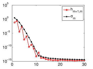
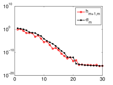
Figure 1: Behavior of the sequences $\left\{h_{m+1,m}\right\}_{m}$ and $\left\{\sigma_{m}\right\}_{m}$ for the test problems baart (left) and shaw (right) from [8].

The following result follows immediately from Theorem 2 and (23).

Corollary 3.

Under the hypothesis of Theorem 2, assume that there exist $M$ such that for $m\leq N$

$$\left|e_{m}^{T}H_{m}^{-1}c\right|\leq M,$$ (25)

where $c=\|b\|e_{1}\in\mathbb{R}^{m}$. Then the GMRES residuals are of the type

$$\left\|r_{m}^{ex}\right\|=O\left(m^{3/2}\sigma_{m}\right).$$ (26)

Employing the SVD of the matrix $H_{m}$, that is, $H_{m}=U_{m}^{(m)}\Sigma_{m}^{(m)}\left(V_{m}^{(m)}\right)^{T}$, $\Sigma_{m}^{(m)}=\mathrm{diag}(\sigma_{1}^{(m)},...,\sigma_{m}^{(m)})$, we have

$$H_{m}^{-1}c=V_{m}^{(m)}(\Sigma_{m}^{(m)})^{-1}U_{m}^{(m)T}c,$$

so that (25) is satisfied as soon as the Discrete Picard Condition is inherited in some way by the projected problem. It is known that if $\widetilde{\sigma}_{j}^{(m)}$, $j=1,...,m$, are the singular values approximations arising from the SVD of $\bar{H}_{m}$, then $\widetilde{\sigma}_{m}^{(m)}\geq\widetilde{\sigma}_{m+1}^{(m+1)}\geq\sigma_{N}>0$ (cf. [3]). Since $h_{m+1,m}$ goes rapidly to 0, we also have that after a few iterations $\sigma_{j}^{(m)}\approx\widetilde{\sigma}_{j}^{(m)}$ so that we can expect that $\sigma_{m}^{(m)}\geq\sigma_{N}$. In general, however, we do not have guarantees that $M$ is small, so that (26) may be quantitatively not much useful. Everything is closely related to the SVD approximation that we can achieve with the Arnoldi algorithm (see [18] for some theoretical results). It is known that if the matrix $A$ is highly nonsymmetric, then the SVD approximation may be poor so that the Discrete Picard Condition may be badly inherited by the projected problem. Anyway, in Figure 2 we report the FOM residual history for some test problems which confirm the behavior described by (26).

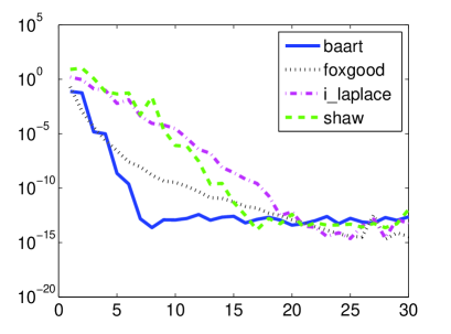
Figure 2: FOM residual history for some common test problems taken from [8].

4.2 The perturbed problem

When the right-hand side of (1) is affected by noise, we can give the following preliminary estimate for the norm of the GMRES residual.

Proposition 4.

Let $b=b^{ex}+e$ and let $r_{m}^{ex}=p_{m}^{ex}(A)b^{ex}$ be the residual of the GMRES applied to the system $Ax=b^{ex}$. Assume that for $m\geq m^{\ast}$, $\left\|p_{m}^{ex}(A)\right\|\leq\eta^{\ast}$. Then the $m$-th residual of the GMRES applied to $Ax=b$ satisfies

$$\left\|r_{m}\right\|\leq\eta\|e\|,$$

where

$$\eta=\frac{\left\|r_{m^{\ast}}^{ex}\right\|}{\|e\|}+\eta^{\ast}.$$

Proof.

Since $b=b^{ex}+e$ and, thanks to the optimality property of the GMRES residual,

$$\left\|r_{m}\right\|=\min_{p_{m}(0)=1}\left\|p_{m}(A)b\right\|\leq\left\|p_{m}^{ex}(A)b\right\|,$$

and hence

$$\left\|r_{m}\right\|\leq\left\|p_{m}^{ex}(A)b^{ex}\right\|+\left\|p_{m}^{ex}(A)e\right\|\leq\left\|r_{m}^{ex}\right\|+\eta^{\ast}\|e\|.$$

The result follows from $\left\|r_{m}^{ex}\right\|\leq\left\|r_{m^{\ast}}^{ex}\right\|$, which holds for $m\geq m^{\ast}$. ∎

In the remaining part of this section, we try to give some additional information about the value of the constant $\eta$ of Proposition 4. Let

$$\widetilde{V}_{m}=\left[\frac{b}{\left\|b\right\|},\frac{Ab}{\left\|Ab\right\|},...,\frac{A^{m-1}b}{\left\|A^{m-1}b\right\|}\right],\quad\widetilde{V}_{m}^{ex}=\left[\frac{b^{ex}}{\left\|b^{ex}\right\|},\frac{Ab^{ex}}{\left\|Ab^{ex}\right\|},...,\frac{A^{m-1}b^{ex}}{\left\|A^{m-1}b^{ex}\right\|}\right].$$

With this notations we can write

$$\left\|r_{m}\right\|=\min_{s\in\mathbb{R}^{m+1},s_{1}=0}\left\|b-\widetilde{V}_{m+1}s\right\|,$$

where $s_{1}$ is the first component of vector $s$.

Proposition 5.

For the GMRES residual we have

$$\left\|r_{m}\right\|\leq\eta(m)\|e\|,$$

where

$$\eta(m)=1+\frac{\left\|r_{m}^{ex}\right\|+\left\|\left(\widetilde{V}_{m+1}-\widetilde{V}_{m+1}^{ex}\right)s^{ex}\right\|}{\left\|e\right\|},$$

in which $s^{ex}$ ($s_{1}^{ex}=0$) is such that $\left\|r_{m}^{ex}\right\|=\left\|b-\widetilde{V}_{m+1}^{ex}s^{ex}\right\|$.

Proof.

We have

$$\left\|r_{m}\right\| = \min_{s\in\mathbb{R}^{m}}\left\|b-\widetilde{V}_{m+1}s\right\|\leq\left\|b-\widetilde{V}_{m+1}s^{ex}\right\|$$

$$= \left\|b^{ex}+e-\widetilde{V}_{m+1}s^{ex}+\widetilde{V}_{m+1}^{ex}s^{ex}-\widetilde{V}_{m+1}^{ex}s^{ex}\right\|$$

$$\leq \left\|r_{m}^{ex}\right\|+\left\|e\right\|+\left\|\left(\widetilde{V}_{m+1}-\widetilde{V}_{m+1}^{ex}\right)s^{ex}\right\|.$$

∎

The fast decay of the singular values of $A$ ensures that, for $k\geq 1$ (note that $s_{1}^{ex}=0$)

$$\frac{1}{\left\|e\right\|}\left\|\frac{A^{k}b}{\left\|A^{k}b\right\|}-\frac{A^{k}b^{ex}}{\left\|A^{k}b^{ex}\right\|}\right\|\ll 1,$$ (27)

so that, whenever $\left\|r_{m}^{ex}\right\|\approx 0$, we have $\eta(m)\approx 1$. Condition (27) is also at the basis of the so-called range-restricted approach for Krylov type methods (see [14]). We also remark that the relation (27) can be interpreted as the discrete analogous of the Riemann-Lebesgue Lemma (see e.g. [9, p.6]), whenever we assume that the noise $e$ does not involve low frequencies. We give some examples of this behavior in Figure 3.

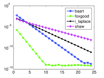
Figure 3: Decay of the quantities $\frac{1}{\|e\|}\left\|\frac{A^{k}b}{\left\|A^{k}b\right\|}-\frac{A^{k}b^{ex}}{\left\|A^{k}b^{ex}\right\|}\right\|$ versus the value of $k\geq 1$. The right-hand side is affected by 1% Gaussian noise.

Finally, in Figure 4 we prove experimentally our main assumption, that is, $\left\|r_{m}\right\|\approx\left\|e\right\|$ for $m$ sufficiently large, which justifies the use of formula (22).

.

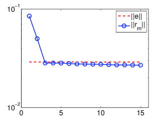
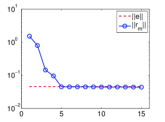
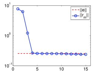
Figure 4: GMRES residual history when the right-hand side is affected by 1% noise. In clockwise order the problem considered are baart, foxgood, shaw and i_laplace

5 Algorithm and Numerical Experiments

Comparing the parameter selection strategies (21) and (22), we can state that (22) generalizes the approach described in Section 3, since no knowledge of $\|e\|$ is assumed. However, on the downside, scheme (21) can simultaneously determine the value of the regularization parameter at each iteration and the number of iterations to be performed, while this is no more possible considering the rule (22). In order to determine when to stop the iterations of the Arnoldi algorithm, we have to consider a separate stopping criterion. Since both $\phi_{m}(\lambda_{m-1})$ and $\|r_{m}\|$ exhibit a stable behavior going on with the iterations, a way to set $m$ is to monitor when such stability occurs, i.e., to evaluate the relative difference between the norm of the residuals and the relative difference between the discrepancy functions. Therefore, once two thresholds $\tau_{\mathrm{res}}$ and $\tau_{\mathrm{discr}}$ have been set, we decide to stop the iterations as soon as

$$\frac{\|r_{m}\|-\|r_{m-1}\|}{\|r_{m-1}\|}<\tau_{\mathrm{res}},$$ (28)

and

$$\frac{\phi_{m}(\lambda_{m-1})-\phi_{m-1}(\lambda_{m-2})}{\phi_{m-1}(\lambda_{m-2})}<\tau_{\mathrm{discr}}.$$ (29)

This approach is very similar to the one adopted in [4] for the GCV method in a hybrid setting. Also in [3] the authors decide to terminate the Arnoldi process when the corners of two consecutive projected L-curves are pretty close. We can also expect the value of $\lambda_{m}$ obtained at the end of the iterations to be suitable for the original problem (4).

The method so far described, can be summarized in the following

Algorithm 1 AT method equipped with the parameter choice rule (22)

Inputs: $A$, $b$, $L$, $x_{0}$, $\lambda_{0}$, $\eta$, $\tau_{\mathrm{res}}$, $\tau_{\mathrm{discr}}$

For $m=1,2,\dots,$ until (28) and (29) are both fulfilled

1. Update $W_{m}$ and $\bar{H}_{m}$ by the Arnoldi algorithm (9).

2. Compute the reduced-dimension GMRES solution $y_{m,0}$ (cf. (10) and the corresponding residual $r_{m}$.

3. Compute the solution $y_{m,\lambda}$ of (14), taking

   $$\begin{cases}\lambda=\lambda_{0}&\mathrm{if}\>m=1,2,\\ \lambda=\lambda_{m-1}&\mathrm{otherwise.}\end{cases}.$$

4. Compute the discrepancy $\phi_{m}(\lambda_{m-1})=\|\bar{H}_{m}y_{m,\lambda_{m-1}}-c\|$.

5. if $m\geq 2$ update $\lambda_{m}$ by formula (22).

end

Compute $x_{m,\lambda_{m-1}}=W_{m}y_{m,\lambda_{m-1}}$.

To illustrate the behavior of this algorithm, we treat three different kinds of test problems. All the experiments have been carried out using Matlab 7.10 with $16$ significant digits on a single processor computer (Intel Core i7). The algorithm is implemented with $\lambda_{0}=1$, $\eta=1.02$, and $\tau_{\mathrm{res}}=\tau_{\mathrm{discr}}=5\cdot 10^{-2}$.

5.1 Test problems from Regularization Tools

We consider again some classical test problems taken from Hansen’s Regularization Tools [8]. In particular in Figure 5, we report the results for the problems baart, shaw, foxgood, i_laplace; the right-hand side $b$ is affected by additive 0.1% Gaussian noise $e$, such that the noise level $\varepsilon=\|e\|/\|b^{ex}\|$ is equal to $10^{-3}$. The dimension of each problem is $N=120$. The regularization operator used is the discrete first derivative $L_{1}$ for shaw and i_laplace, and the discrete second derivative $L_{2}$ for baart and foxgood, augmented with one or two zero rows respectively, in order to make it square, that is,

$$L_{1}:=\left(\begin{array}[]{cccc}1&-1&&\\ &\ddots&\ddots&\\ &&1&-1\\ 0&...&...&0\end{array}\right),\quad L_{2}:=\left(\begin{array}[]{ccccc}1&-2&1&&\\ &\ddots&\ddots&\ddots&\\ &&1&-2&1\\ 0&...&...&...&0\\ 0&...&...&...&0\end{array}\right).$$ (30)

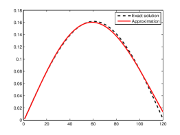
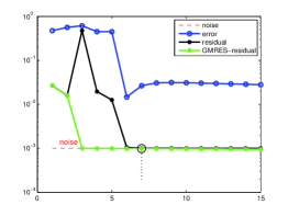
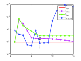
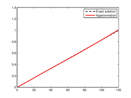
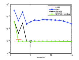
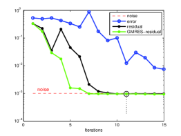
Figure 5: From top to bottom: results for baart, foxgood, i_laplace, shaw. On the left column we display the computed approximate solution. In the middle column we show the convergence behavior of the new method (error, discrepancy and GMRES residual) with the noise level highlighted by a dashed lines. On the right we compare different parameter choice strategies. The tick circle displayed in all the frame of the middle and the rightmost columns marks the iteration at which we would stop, according to the rule (28), (29). The approximate solutions refer to this iteration.

For each experiment we show: a) the approximate solution; b) the relative residual and error history; c) the value of the regularization parameter computed at each iteration by the secant update method ($\lambda_{\mathrm{sec}}$) given by formula (21), the embedded method ($\lambda_{\mathrm{emb}}$) computed by (22), the ones arising from the L-curve criterion ($\lambda_{\mathrm{L-curve}}$) see [3], and the optimal one ($\lambda_{\mathrm{opt}}$) for the original, full-dimensional regularized problem (4) obtained by the minimization of the distance between the regularized and the exact solution [19]

$$\min_{\lambda}\left\|x_{\lambda}-x^{ex}\right\|^{2}=\min_{\lambda}\left\|\sum_{i=1}^{P}\frac{\lambda^{2}}{(\gamma_{i}^{2}+\lambda^{2})}\frac{\bar{u}_{i}^{T}b}{\sigma_{i}}x_{i}+\sum_{i=P+1}^{N}(u_{i}^{T}b)x_{i}-\sum_{i=1}^{N}\frac{u_{i}^{T}b^{ex}}{\sigma_{i}}v_{i}\right\|,$$

where $\gamma_{i}$, $\bar{u}_{i}$, $i=1,\dots,P$ are respectively the generalized singular values and left generalized singular vectors of $(A,L)$, and $x_{i}$, $i=1,\dots,N$ are the right generalized singular vectors of $(A,L)$.

5.2 Results for Image Restoration

To test the performance of our algorithm in the image restoration contest, a number of experiments were carried out, some of which are presented here.

Let $X$ be a $n\times n$ two dimensional image. The vector $x^{ex}$ of dimension $N=n^{2}$ obtained by stacking the columns of the image $X$ and the associated blurred and noise-free image $b^{ex}$ is generated by multiplying $x^{ex}$ by a blurring matrix $A\in\mathbb{R}^{N\times N}$. The matrix $A$ is block Toeplitz with Toeplitz blocks and is implemented in the function blur from [8], which has two parameters, band and sigma; the former specifies the half-bandwidth of the Toeplitz blocks and the latter the variance of the Gaussian point spread function. We generate a blurred and noisy image $b\in\mathbb{R}^{N}$ by adding a noise-vector $e\in\mathbb{R}^{N}$, so that $b=Ax^{ex}+e$. We assume the blurring operator $A$ and the corrupted image $b$ to be available while no information is given on the error $e$.

In the example, the original image is the cameraman.tif test image from Matlab, a $256\times 256$, 8-bit gray-scale image, commonly used in image deblurring experiments. The image is blurred with parameters band=7 and sigma=2. We further corrupt the blurred images with 0.1% additive Gaussian noise. The blurred and noisy image is shown in the center column of Figure 6, the regularization operator is defined as

$$L=I_{n}\otimes L_{1}+L_{1}\otimes I_{n}\in\mathbb{R}^{N\times N},$$ (31)

(cf. [12, §5]). The restored image is shown in the right column of Figure 6 . The result has been obtained in $m=8$ iterations of the Arnoldi algorithm, the CPU-time required for this experiment is around $1.2$ seconds. Many other experiments on image restoration have shown similar performances.

Figure 6: Restoration of cameraman.tif. From left to right: original image; blurred and noisy image with blur parameters band=7, sigma=2 and noise level $\varepsilon=10^{-3}$; restored image. From top to bottom: original-size image and two zooms.

5.3 Results for MRI Reconstruction

The treatment of different kinds of medical images such as Magnetic Resonance Imaging (MRI), Computed Tomography (CT), Position Emission Tomography (PET), often requires the usage of image processing techniques to remove various types of degradations such as noise, blur and contrast imperfections. Our experiments focus on MRI medical image affected by Gaussian blur and noise. Typically, when blur and noise affect the MRI images, the visibility of small components in the image decreases and therefore image deblurring techniques are extensively employed to grant the image a sharper appearance.

In our test we blur a synthetic MRI $256\times 256$ image, with Gaussian blur (band=9, sigma=2.5), and we add 10% Gaussian white noise, since the noise level of a real problem may be expected to be quite high.

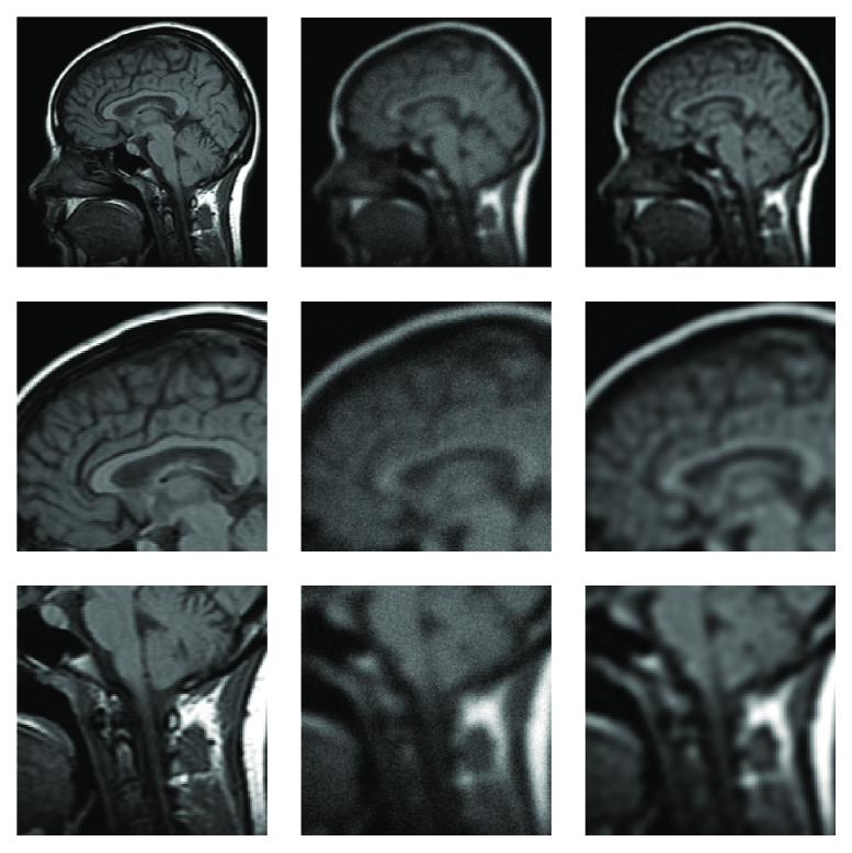
Figure 7: Restoration of the test image mri.png image. From left to right: original image; blurred and noisy image with noise level $\varepsilon=10^{-1}$ and blur parameters band=9, sigma=2.5; restored image. From top to bottom original size image and two zooms.

Figure 7 displays the performance of the algorithm. On the left column we show the blur-free and noise-free image, on the middle column we show the corrupted image, on the right column we show the restored image.The regularization operator employed is again (31). The result has been obtained in $m=5$ iterations of the algorithm, in around $0.7$ seconds.

6 Conclusions

In this paper we have proposed a very simple method to define the sequence of regularization parameters for the Arnoldi Tikhonov method, in absence of information on the percentage of error which affects the right hand side. The numerical results have shown that this technique is rather stable, with results comparable with the existing approaches (GCV, L-curve). We have used the term ”embedded” to describe this procedure since the construction of the Krylov subspaces is used, at the same time, either as error estimator by means of the GMRES residual or for the solution of (4) with the AT method. We remark that, in principle, the idea can be applied to any basic iterative method able to approximate $\left\|e\right\|$ and, at the same time, usable in connection with Tikhonov regularization (as for instance, probably, the Lanczos bidiagonalization).

7 Appendix

While, in general, the SVD decomposition can be considered independent of the Arnoldi process in absence of hypothesis on the starting vector $b$, the following proposition states that, if the Discrete Picard Condition is satisfied, then we are able to express a relation between $R(U_{m})$ (the space generated by the columns of $U_{m}$, where $U_{m}\Sigma_{m}V_{m}^{T}$ is the truncated SVD of $A$) and $\mathcal{K}_{m}(A,b)$. In order to reduce the complexity of the notations, with respect to Section 4 here $b$ simply denotes the unperturbed right-hand side of the system.

Proposition 6.

Assume that the singular values $A$ are of the type $\sigma_{j}=O(e^{-\alpha j})$ ($\alpha>0$). Assume moreover that the Discrete Picard Condition is satisfied. Let $\widetilde{V}_{m}:=\left[\widetilde{v}_{0},...,\widetilde{v}_{m-1}\right]\in\mathbb{R}^{N\times m}$ where $\widetilde{v}_{k}:=A^{k}b/\left\|A^{k}b\right\|$. If $\widetilde{V}_{m}$ has full column rank, then there exist $C_{m}\in\mathbb{R}^{m\times m}$ nonsingular, $E_{m},F_{m}\in\mathbb{R}^{N\times m}$, such that

$$\widetilde{V}_{m} = U_{m}C_{m}+E_{m},\quad\left\|E_{m}\right\|=O(m^{1/2}\sigma_{m}),$$ (32)

$$U_{m} = \widetilde{V}_{m}C_{m}^{-1}+F_{m},\quad\left\|F_{m}\Sigma_{m}\right\|=O(m^{3/2}\sigma_{m}).$$ (33)

Proof.

Let $U_{m}^{\perp}:=\left[u_{m+1},...,u_{N}\right]\in\mathbb{R}^{N\times(N-m)}$. Defining $C_{m}:=U_{m}^{T}\widetilde{V}_{m}\in\mathbb{R}^{m\times m}$ and $E_{m}:=U_{m}^{\perp}\left(U_{m}^{\perp}\right)^{T}\widetilde{V}_{m}\in\mathbb{R}^{N\times m}$ we have $\widetilde{V}_{m}=U_{m}C_{m}+E_{m}$. Now we observe that for $0\leq k\leq m-1$

$$\left|u_{j}^{T}\widetilde{v}_{k}\right|\sim\sigma_{j}.$$ (34)

For $k=0$ the above relation is ensured by the Picard Condition, whereas for $k\geq 1$ it holds since

$$\widetilde{v}_{k}=\frac{\left\|A^{k-1}b\right\|}{\left\|A^{k}b\right\|}A\widetilde{v}_{k-1}.$$

Therefore, using $\sigma_{j}=O(e^{-\alpha j})$, we immediately obtain

$$\left\|E_{m}\right\|=\left\|\left(U_{m}^{\perp}\right)^{T}\widetilde{V}_{m}\right\|=O(m^{1/2}\sigma_{m}),$$ (35)

We observe that the matrix $C_{m}$ can be written as

$$C_{m}=U_{m}^{T}W_{m}S_{m},$$

where $S_{m}$ is upper triangular and nonsingular if $\widetilde{V}_{m}$ has full rank. Now, from the relation [6, §2.6.3]

$$\sigma_{\min}(U_{m}^{T}W_{m})^{2}=1-\left\|\left(U_{m}^{\perp}\right)^{T}W_{m}\right\|^{2},$$

the quantity $\left\|\left(U_{m}^{\perp}\right)^{T}W_{m}\right\|$, which express the distance between $R(U_{m})$ and $R(W_{m})$, is strictly less than one if the Picard Condition is satisfied. Thus, by (32), we can write

$$U_{m}=\widetilde{V}_{m}C_{m}^{-1}-E_{m}C_{m}^{-1},$$ (36)

and since $E_{m}=U_{m}^{\perp}\left(U_{m}^{\perp}\right)^{T}\widetilde{V}_{m}$ we have that

$$E_{m}C_{m}^{-1}=U_{m}^{\perp}\left(U_{m}^{\perp}\right)^{T}\widetilde{V}_{m}\left(U_{m}^{T}\widetilde{V}_{m}\right)^{-1}.$$ (37)

By (34), using the Cramer rule to compute $\left(U_{m}^{T}\widetilde{V}_{m}\right)^{-1}\Sigma_{m}\in\mathbb{R}^{m\times m}$ we can see that each element of this matrix is of the type $O(1)$, so that

$$\left|\left(U_{m}^{\perp}\right)^{T}\widetilde{V}_{m}\left(U_{m}^{T}\widetilde{V}_{m}\right)^{-1}\Sigma_{m}\right|\sim m\left(\begin{array}[]{ccc}\sigma_{m+1}&\cdots&\sigma_{m+1}\\ \vdots&&\vdots\\ \sigma_{N}&\cdots&\sigma_{N}\end{array}\right)\in\mathbb{R}^{(N-m)\times m},$$

and hence

$$\left\|\left(U_{m}^{\perp}\right)^{T}\widetilde{V}_{m}\left(U_{m}^{T}\widetilde{V}_{m}\right)^{-1}\Sigma_{m}\right\|=O(m^{3/2}\sigma_{m}),$$ (38)

using again $\sigma_{j}=O(e^{-\alpha j})$. Defining $F_{m}=-E_{m}C_{m}^{-1}$ we obtain (33) by (36), (37) and (38). ∎

Thanks to the above Proposition, the following proof of Theorem 2 stated in Section 4.1 is straightforward.

Proof of Theorem 2. Let $A_{m}=U_{m}\Sigma_{m}V_{m}^{T}$, and let $\Delta_{m}=A-A_{m}$. By (9)

$$h_{m+1,m} = w_{m+1}^{T}Aw_{m}$$

$$= w_{m+1}^{T}\Delta_{m}w_{m}+w_{m+1}^{T}A_{m}w_{m}$$

$$= O(\sigma_{m+1})+w_{m+1}^{T}U_{m}\Sigma_{m}V_{m}^{T}w_{m},$$

since $\left\|\Delta_{m}\right\|=\sigma_{m+1}$. Therefore, using (33) we obtain

$$h_{m+1,m}=O(\sigma_{m+1})+w_{m+1}^{T}(\widetilde{V}_{m}C_{m}^{-1}+F_{m})\Sigma_{m}V_{m}^{T}w_{m}.$$

which concludes the proof, since $w_{m+1}^{T}\widetilde{V}_{m}=0$ and $\left\|F_{m}\Sigma_{m}\right\|=O(m^{3/2}\sigma_{m})$.                   $\square$

Remark 7.

The hypothesis $\sigma_{j}=O(e^{-\alpha j})$ apparently limits the above results to severely ill-conditioned problems. Actually, it is just used in (35) and (38) since, by the integral criterion,

$$\sum\nolimits_{j\geq m+1}\sigma_{j}=O(e^{-\alpha m})=O(\sigma_{m}).$$

In this sense, the results can be extended to mildly ill-conditioned problems, in which $\sigma_{j}=O(j^{-\alpha})$, $\alpha>1$. In this situation we would have

$$\sum\nolimits_{j\geq m+1}\sigma_{j}=O(m^{1-\alpha}),$$

so that, for $\alpha$ sufficiently large, (32), (33) and the results of Theorem 2 and Corollary 3, can be extended to mildly ill-conditioned problems by replacing $\sigma_{m}$ with $O(m^{1-\alpha})$.

References

- [1] F. Bauer, M. Lukas, Comparing parameter choice methods for regularization of ill-posed problems, Math. Comput. Simulation 81 (9)(2011), pp. 1795–1841.
- [2] D. Calvetti, B. Lewis, L. Reichel, On the regularizing properties of the GMRES method, Numer. Math. 91 (2002), pp. 605–625.
- [3] D. Calvetti, S. Morigi, L. Reichel, F. Sgallari, Tikhonov regularization and the L-curve for large discrete ill-posed problems, J. Comput. Appl. Math. 123 (2000), pp. 423–446.
- [4] J. Chung, J.G. Nagy, D.P. O’Leary, A weighted-GCV method fo Lanczos-hybrid regularization, ETNA 28 (2008), pp. 149–167.
- [5] S. Gazzola, P. Novati, Automatic parameter setting for Arnoldi-Tikhonov methods, submitted (2012).
- [6] G.H. Golub, C.F. Van Loan, Matrix Computations. Johns Hopkins University Press, Baltimore (MD), 3rd edition, 1996.
- [7] P.C. Hansen, The Discrete Picard Condition for Discrete Ill-Posed Problems, BIT 30 (1990), pp. 658–672.
- [8] P.C. Hansen, Regularization Tools: A Matlab package for analysis and solution of discrete ill-posed problems, Numer. Algorithms 6 (1994), pp. 1–35.
- [9] P.C. Hansen, Rank-Deficient and Discrete Ill-Posed Problems. Numerical Aspects of Linear Inversion. SIAM, Philadelphia (PA), 1998.
- [10] M. Hochstenbach and L. Reichel, An iterative method for Tikhonov regularization with a general linear regularization operator, J. Integral Equations Appl. 22 (2010), pp. 463–480.
- [11] B. Hofmann, Regularization for Applied Inverse and Ill-Posed Problems. Teubner, Stuttgart (Germany), 1986.
- [12] M.E. Kilmer, P.C. Hansen, M.I. Español, A projection-based approach to general-form Tikhonov regularization, SIAM J. Sci. Comput. 29(1) (2007), 315–330.
- [13] M.E. Kilmer, D.P. O’Leary, Choosing regularization parameters in iterative methods for ill-posed problems, SIAM J. Matrix Anal. Appl. 22 (2001), pp. 1204–1221.
- [14] B. Lewis, L. Reichel, Arnoldi-Tikhonov regularization methods, J. Comput. Appl. Math. 226 (2009), pp. 92–102.
- [15] G. Meurant, On the residual norm in FOM and GMRES, SIAM J. Matrix Anal. Appl. 32 (2011), pp. 394–411.
- [16] I. Moret, A note on the superlinear convergence of GMRES, SIAM J. Numer. Anal. 34(2) (1997), pp. 513–516.
- [17] P. Novati, M.R. Russo, Adaptive Arnoldi-Tikhonov regularization for image restoration, to appear in Numer. Algorithms (2013), doi:10.1007/s11075-013-9712-0[1].
- [18] P. Novati, M.R. Russo, A GCV based Arnoldi-Tikhonov regularization method, submitted (2013), http://arxiv.org/abs/1304.0148.
- [19] D.P. O’Leary, Near-optimal parameters for Tikhonov and other regularization methods, SIAM J. Sci. Comput. 23(4) (2001), 1161–1171.
- [20] D.P. O’Leary, J.A. Simmons, A bidiagonalization-regularization procedure for large-scale discretizations of ill-posed problems, SIAM J. Sci. Statist. Comput. 2 (1981), pp. 474–489.
- [21] L. Reichel, G. Rodriguez, Old and new parameter choice rules for discrete ill-posed problems, Numer. Algorithms 63 (2013), pp. 65–87.
- [22] L. Reichel, A. Shyshkov, A new zero-finder for Tikhonov regularization, BIT 48 (2008), pp. 627–643.
- [23] Y. Saad, Iterative methods for Sparse Linear Systems, 2nd edition, SIAM, Philadelphia (PA), 2003.