Energy transfer using unitary transformations

Abstract

We study the unitary time evolution of a simple quantum Hamiltonian describing two harmonic oscillators coupled via a three-level system. The latter acts as an engine transferring energy from one oscillator to the other and is driven in a cyclic manner by time-dependent external fields. The $S$-matrix of the cycle is obtained in analytic form. The total number of quanta contained in the system is a conserved quantity. As a consequence the spectrum of the $S$-matrix is purely discrete and the evolution of the system is quasi-periodic.

1 Introduction

The use of a three level system as an engine to transfer energy between two quantum systems has been proposed half a century ago by Scovil and Schulz-Dubois [1, 2]. The population of the levels can be manipulated using light pulses. In particular, the Stimulated Raman Adiabatic Passage (STIRAP) technique [3, 4, 5] has become a very efficient experimental tool [6]. The three-level system is brought in contact alternatingly with the system of interest and with an energy reservoir, called the heat bath. In this way energy can be removed from the system under study.

Quantum entanglement between the system and the heat bath is usually neglected. It is assumed to be suppressed by decoherence phenomena active in the heat bath. In the present model both the system and the reservoir consist of single harmonic oscillators. These are too simple to cause decoherence. One can therefore expect that quantum entanglement is dominantly present. The importance of the entanglement of system and reservoir has been stressed recently [7].

The thermal state of the system is usually described by a density matrix. Here we deviate from this tradition by assuming that the state of our three component system is described by a time-dependent wave function $\psi$ which is a solution of the Schrödinger equation. It is a closed system in the sense that the time evolution is unitary and deterministic. This corresponds experimentally with an operation on a time scale which is short compared to the time scale of thermal equilibration.

The model is introduced in the next Section. The $S$-matrix approach is explained in Section 3. The analytic expression for the $S$-matrix corresponding with one cycle of the engine is obtained. In Section 4 we analyze our results. Final conclusions follow in Section 5. The details of our calculations are explained in the Appendices.

2 The model

The model Hamiltonian $H$ consists of an unperturbed part $H_{0}$ describing two harmonic oscillators (HO) and an engine, to which are added time-dependent external fields operating the engine and time-dependent interactions between the oscillators and the engine. For convenience, one of the oscillators is called the cold HO, the other the warm HO. The engine is operated in such a way that an energy transfer from cold to warm is expected.

All together, the unperturbed Hamiltonian reads (we use units in which $\hbar=1$)

$$H_{0}=\omega_{1}a^{\dagger}a+H_{gef}+\omega_{3}c^{\dagger}c.$$ (1)

The operators $a$ and $c$ are the annihilation operators of the cold HO and of the warm HO, respectively. The Hamiltonian of the three level system is given by

$$H_{\rm gef}=\left(\begin{array}[]{lcr}-\mu&0&0\\ 0&\mu&0\\ 0&0&\mu+2\delta\end{array}\right).$$ (5)

The three levels are labeled $g$, $e$, and $f$, and have energies $-\mu$, $\mu$, and $\mu+2\delta$, respectively.

The engine is operated by means of a rather primitive sequence of two square pulses. More realistic pulses can be treated analytically as well [8] but would complicate our analysis of the coupled system as a whole. Their contribution is

$$I_{\rm gef}=-\epsilon_{a}(t)\Lambda_{1}-\epsilon_{b}(t)\Lambda_{6},$$ (6)

where $\Lambda_{1}$ and $\Lambda_{6}$ are the Gell-Mann matrices — see the Appendix A.

The interaction between the three level system and each of the harmonic oscillators is inspired by the Jaynes-Cummings model. It describes an exchange of one quantum of energy between a HO and a two-level system. Important for the present work is that its eigenvalues and eigenvectors can be calculated analytically.

The coupling at the cold side is given by

$$H_{12}=\kappa_{12}(t)\big{(}a^{\dagger}E_{+}+aE_{-}\big{)}$$ (7)

with

$$E_{+} = \frac{1}{2}(\Lambda_{1}+i\Lambda_{2})=\left(\begin{array}[]{lcr}0&1&0\\ 0&0&0\\ 0&0&0\end{array}\right)\quad\mbox{ and }$$ (11)

$$E_{-} = \frac{1}{2}(\Lambda_{1}-i\Lambda_{2})=\left(\begin{array}[]{lcr}0&0&0\\ 1&0&0\\ 0&0&0\end{array}\right).$$ (15)

It couples the $g$ and $e$ levels of the three level system. At the warm side the interaction Hamiltonian is given by

$$H_{23}=\kappa_{23}(t)\big{(}F_{+}c^{\dagger}+F_{-}c\big{)}$$ (16)

with

$$F_{+} = \frac{1}{2}(\Lambda_{6}+i\Lambda_{7})=\left(\begin{array}[]{lcr}0&0&0\\ 0&0&1\\ 0&0&0\end{array}\right)\quad\mbox{ and }$$ (20)

$$F_{-} = \frac{1}{2}(\Lambda_{6}-i\Lambda_{7})=\left(\begin{array}[]{lcr}0&0&0\\ 0&0&0\\ 0&1&0\end{array}\right).$$ (24)

It couples the $e$ and $f$ levels of the three level system with the warm HO. The total time-dependent Hamiltonian is now

$$H=H_{0}+H_{12}+I_{\rm gef}+H_{23}.$$ (25)

3 Cycles

The external field strengths $\epsilon_{a}(t)$ and $\epsilon_{b}(t)$ and the coupling parameters $\kappa_{12}(t)$ and $\kappa_{23}(t)$ all depend on time $t$. They are pulsed one after another in such a way that a (not necessary closed) cycle is traversed. See the Figure 1.

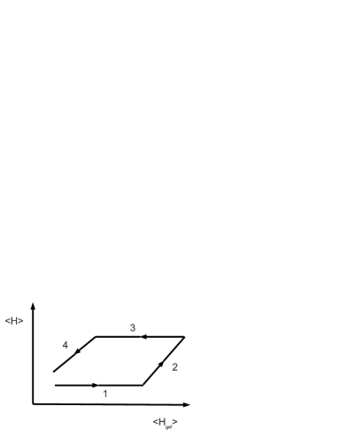
Figure 1: The 4 phases of the cycle. On the horizontal axis is the energy of the engine. On the vertical axis is the total energy of the system.

The cycle starts by coupling the engine to the cold HO. The switching on and off changes the total energy of the system (this contribution is omitted in the figure). But during the first phase of the cycle the total energy is constant. In the second phase the energy of the engine is pumped up by applying a sequence of two pulses. Work is performed by doing so. In phase 3 the engine releases energy to the warm oscillator. In phase 4 the engine delivers work to the environment. This is again modeled by two externally applied pulses which pump down the internal energy of the engine.

Note that the cycle does not necessarily close. It is obvious that in the energy transfer mode the engine will consume more work (during phase 2) than it can deliver (during phase 4). Because the system is finite this implies that the total energy goes up after every cycle of the process. See the Figure 2.

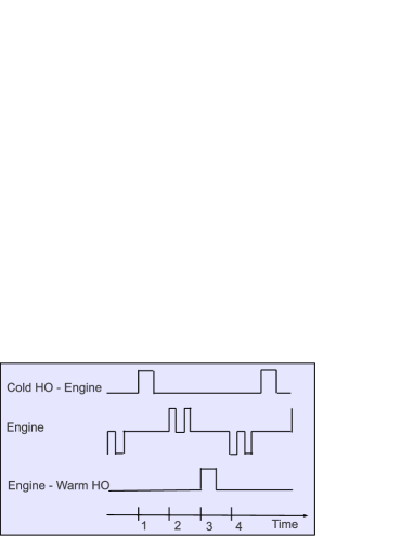
Figure 2: Overview of the activation of the time-dependent terms in the Hamiltonian.

The $S$-matrix approach

The time evolution of the system with Hamiltonian (25) is studied without making crude approximations. The calculation is simplified by the use of the interaction picture. Then the wave function of the total system — engine plus oscillators — is time-independent in the periods when none of the time-dependent terms is active. The effect of activating one of the interaction terms or one of the external fields is then to transform the wave function $\psi$ by means of an S-matrix into a new wave function $S\psi$.

Step 1: Absorbing energy from the cold HO

In the first phase of the cycle the three level system is connected to the cold HO during a time $\tau_{1}$. The corresponding S-matrix is denoted $S_{1}$. It is not very difficult to calculate it exactly. See the Appendix B. The result is of the form

$$S_{1} = e^{i\tau_{1}H_{0}}e^{-i\tau_{1}H}$$ (26)

$$= e^{\frac{i}{2}\tau_{1}(\omega_{1}-2\mu)}\left[a^{\dagger}(A-iC)aE_{1}+ia^{\dagger}BE_{+}\right]$$ (29)

$$+e^{-\frac{i}{2}\tau_{1}(\omega_{1}-2\mu)}\left[iBaE_{-}+aa^{\dagger}(A+iC)E_{2}\right]$$

$$+G_{1}E_{1}+E_{3},$$

with

$$E_{1} = E_{+}E_{-}=\left(\begin{array}[]{lcr}1&0&0\\ 0&0&0\\ 0&0&0\\ \end{array}\right),\quad E_{2}=E_{-}E_{+}=\left(\begin{array}[]{lcr}0&0&0\\ 0&1&0\\ 0&0&0\\ \end{array}\right),$$ (36)

$$E_{3} = \left(\begin{array}[]{lcr}0&0&0\\ 0&0&0\\ 0&0&1\\ \end{array}\right),$$ (40)

and

$$A = \sum_{n}\frac{1}{n+1}\cos(\tau_{1}\lambda_{n})|n\rangle\langle n|,$$ (41)

$$B = \sum_{n}\frac{1}{\sqrt{n+1}}\sin(\tau_{1}\lambda_{n})\sin(2\theta_{n})|n\rangle\langle n|,$$ (42)

$$C = \sum_{n}\frac{1}{n+1}\sin(\tau_{1}\lambda_{n})\cos(2\theta_{n})|n\rangle\langle n|.$$ (43)

The coefficients $\lambda_{n}$ and the angles $\theta_{n}$ are given by

$$\lambda_{n} = \frac{1}{2}\sqrt{4\kappa_{12}^{2}(n+1)+(\omega_{1}-2\mu)^{2}}$$ (45)

$$\tan(\theta_{n}) = \frac{2\kappa_{12}\sqrt{n+1}}{2\lambda_{n}+\omega_{1}-2\mu}.$$ (46)

The operator $G_{1}$ is the orthogonal projection $|0\rangle\langle 0|$ onto the ground state of the cold HO.

Step 2: Pumping up

We apply a sequence of two pulses of the on/off type. The first pulse is realized by giving $\epsilon_{a}(t)$ a constant non-zero value during a time $\tau_{a}$. It tries to invert the population of the levels $e$ and $f$. The change of the population as a consequence of this pulse is given by the S-matrix $S_{2a}$ which is now calculated.

$$S_{2a} = e^{i\tau_{a}H_{0}}e^{-i\tau_{a}H}$$ (47)

$$= e^{i\tau_{a}H_{\rm gef}}e^{-i\tau_{a}(H_{\rm gef}-\epsilon_{a}\lambda_{6})}$$ (48)

$$= e^{-i\tau_{a}\delta\sigma_{3}}e^{i\tau_{a}[\delta\sigma_{3}-\epsilon_{a}\sigma_{1}]}.$$ (49)

Note that we switched notations, using two-dimensional Pauli matrices instead of the Gell-Mann matrices, omitting one dimension for a moment. Introduce the constant $T_{a}=1/\sqrt{\delta^{2}+\epsilon_{a}^{2}}$. There follows

$$S_{2a} = \left[\cos(\tau_{a}\delta)-i\sin(\tau_{a}\delta)\sigma_{3}\right]$$ (51)

$$\times\left[\cos(\tau_{a}/T_{a})+iT_{a}\sin(\tau_{a}/T_{a})(\delta\sigma_{3}-\epsilon_{a}\sigma_{1})\right].$$

Let us now make an appropriate choice of the pulse duration $\tau_{a}$. The goal is to minimize the population of the $e$-level after the pulse. Since one can expect that before the pulse the $e$-level is more populated than the $f$-level the best one can do is to require that the $e$ matrix element of $S_{2a}$ is as small as possible in modulus. Let therefore $\tau_{a}=\frac{1}{2}\pi T_{a}$. Then the S-matrix becomes

$$S_{2a} = iT_{a}\left[\cos(\tau_{a}\delta)-i\sin(\tau_{a}\delta)\sigma_{3}\right]\sin(\tau_{a}/T_{a})(\delta\sigma_{3}-\epsilon_{a}\sigma_{1}).$$ (53)

Restoring the third dimension this becomes

$$S_{2a} = \left(\begin{array}[]{lcr}1&0&0\\ 0&0&0\\ 0&0&0\end{array}\right)+iT_{a}\left(\begin{array}[]{lcr}0&0&0\\ 0&\delta e^{-i\tau_{a}\delta}&-\epsilon_{a}e^{-i\tau_{a}\delta}\\ 0&-\epsilon_{a}e^{i\tau_{a}\delta}&-\delta e^{i\tau_{a}\delta}\end{array}\right).$$ (60)

In the limit of a strong short pulse this becomes

$$S_{2a} = \left(\begin{array}[]{lcr}1&0&0\\ 0&0&-i\\ 0&-i&0\end{array}\right).$$ (65)

The first pulse of the second phase of the cycle is followed by a pulse of duration $\tau_{b}$, intended to invert the population of levels $e$ and $g$. The corresponding S-matrix reads, using the notation $T_{b}=1/\sqrt{\mu^{2}+\epsilon_{b}^{2}}$,

$$S_{2b} = e^{i\tau_{b}H_{0}}e^{-i\tau_{b}H}$$ (66)

$$= e^{i\tau_{b}H_{\rm gef}}e^{-i\tau_{b}(H_{\rm gef}-\epsilon_{b}\lambda_{1})}$$ (67)

$$= \left[\cos(\tau_{b}\mu)-i\sin(\tau_{b}\mu)\sigma_{3}\right]$$ (69)

$$\times\left[\cos(\tau_{b}/T_{b})+iT_{b}\sin(\tau_{b}/T_{b})(\mu\sigma_{3}+\epsilon_{b}\sigma_{1}\right]$$

With similar arguments as before let us choose $\tau_{b}=\frac{1}{2}\pi T_{b}$. Then the S-matrix becomes

$$S_{2b} = \left(\begin{array}[]{lcr}0&0&0\\ 0&0&0\\ 0&0&1\end{array}\right)+iT_{b}\left(\begin{array}[]{lcr}\mu e^{-i\tau_{b}\mu}&\epsilon_{b}e^{-i\tau_{b}\mu}&0\\ \epsilon_{b}e^{i\tau_{b}\mu}&-\mu e^{i\tau_{b}\mu}&0\\ 0&0&0\end{array}\right).$$ (77)

In the limit of a strong short pulse this becomes

$$S_{2b} = \left(\begin{array}[]{lcr}0&i&0\\ i&0&0\\ 0&0&1\end{array}\right).$$ (81)

All together the S-matrix for the second phase of the cycle equals

$$S_{2} = S_{2b}S_{2a}$$ (82)

$$= \left(\begin{array}[]{lcr}iT_{b}\mu e^{-i\tau_{b}\mu}&-T_{a}T_{b}\epsilon_{b}\delta e^{-i\tau_{a}\delta-i\tau_{b}\mu}&T_{a}T_{b}\epsilon_{a}\epsilon_{b}e^{-i\tau_{a}\delta-i\tau_{b}\mu}\\ iT_{b}\epsilon_{b}e^{i\tau_{b}\mu}&T_{a}T_{b}\mu\delta e^{-i\tau_{a}\delta+i\tau_{b}\mu}&-T_{a}T_{b}\mu\epsilon_{a}e^{-i\tau_{a}\delta+i\tau_{b}\mu}\\ 0&-iT_{a}\epsilon_{a}e^{i\tau_{a}\delta}&-iT_{a}\delta e^{-i\tau_{a}\delta}\end{array}\right).$$ (86)

In the limit of strong short pulses it becomes

$$S_{2} = \left(\begin{array}[]{lcr}0&0&1\\ i&0&0\\ 0&-i&0\end{array}\right).$$ (91)

Step 3: Exchanging energy with the warm oscillator

In the third phase of the cycle the three level system is connected to the warm HO during a time $\tau_{3}$. The corresponding S-matrix is denoted $S_{3}$. The calculation is similar to that in Step 1. The result is of the form

$$S_{3} = e^{i\tau_{3}H_{0}}e^{-i\tau_{3}H}$$ (92)

$$= E_{1}+E_{2}G_{3}$$ (95)

$$+e^{\frac{i}{2}\tau_{3}(\omega_{3}-2\delta)}\left[c^{\dagger}(Z-iV)cE_{2}+ic^{\dagger}YF_{+}\right]$$

$$+e^{-\frac{i}{2}\tau_{3}(\omega_{3}-2\delta)}\left[iYcF_{-}+cc^{\dagger}(Z+iV)E_{3}\right]$$

with

$$Z = \sum_{n}\frac{1}{n+1}\cos(\tau_{3}\xi_{n})|n\rangle\langle n|$$ (96)

$$Y = \sum_{n}\frac{1}{\sqrt{n+1}}\sin(\tau_{3}\xi_{n})\sin(2\phi_{n})|n\rangle\langle n|,$$ (97)

$$V = \sum_{n}\frac{1}{n+1}\sin(\tau_{3}\xi_{n})\cos(2\phi_{n})|n\rangle\langle n|.$$ (98)

The coefficients $\xi_{n}$ and the angles $\phi_{n}$ are given by

$$\xi_{n} = \frac{1}{2}\sqrt{4\kappa_{23}^{2}(n+1)+(\omega_{3}-2\delta)^{2}}$$ (100)

$$\tan(\phi_{n}) = \frac{2\kappa_{23}\sqrt{n+1}}{2\xi_{n}+\omega_{3}-2\delta}.$$ (101)

The operator $G_{3}$ is the orthogonal projection $|0\rangle\langle 0|$ onto the ground state of the warm HO.

Step 4: Pumping down

The operation in the fourth phase is the inverse of that in the second phase. We thus have $S_{4}=S_{2}^{\dagger}$.

4 Analysis

In the previous Section the contribution to the S-matrix from each of the four phases of the cycle has been obtained. The composite matrix $S=S_{4}S_{3}S_{2}S_{1}$ is now calculated. The result is a rather complicated. Therefore a tensor notation is appropriate. Remember that the Hilbert space of wave functions of the total system is the tensor product

$${\cal H}={\cal H}_{\rm cold}\otimes{\mathbb{C}}^{3}\otimes{\cal H}_{\rm warm}.$$ (102)

The first and the last factor are the Hilbert space of the cold and of the warm HO, respectively. The middle factor is the space of vectors with three complex components.

4.1 The composed S-matrix

The full S-matrix reads

$$S = {\mathbb{I}}\otimes S_{2}^{\dagger}\otimes{\mathbb{I}}$$ (103)

$$\times \bigg{\{}{\mathbb{I}}\otimes E_{1}\otimes{\mathbb{I}}+{\mathbb{I}}\otimes E_{2}\otimes G_{3}$$ (106)

$$+e^{\frac{i}{2}\tau_{3}(\omega_{3}-2\delta)}\left[{\mathbb{I}}\otimes E_{2}\otimes c^{\dagger}(Z-iV)c+i{\mathbb{I}}\otimes F_{+}\otimes c^{\dagger}Y\right]$$

$$+e^{-\frac{i}{2}\tau_{3}(\omega_{3}-2\delta)}\left[i{\mathbb{I}}\otimes F_{-}\otimes Yc+{\mathbb{I}}\otimes E_{3}\otimes cc^{\dagger}(Z+iV)\right]\bigg{\}}$$

$$\times {\mathbb{I}}\otimes S_{2}\otimes{\mathbb{I}}$$ (107)

$$\times \bigg{\{}e^{\frac{i}{2}\tau_{1}(\omega_{1}-2\mu)}\left[a^{\dagger}(A-iC)a\otimes E_{1}\otimes{\mathbb{I}}+ia^{\dagger}B\otimes E_{+}\otimes{\mathbb{I}}\right]$$ (110)

$$+e^{-\frac{i}{2}\tau_{1}(\omega_{1}-2\mu)}\left[iBa\otimes E_{-}\otimes{\mathbb{I}}+aa^{\dagger}(A+iC)\otimes E_{2}\otimes{\mathbb{I}}\right]$$

$$+G_{1}\otimes E_{1}\otimes{\mathbb{I}}+{\mathbb{I}}\otimes E_{3}\otimes{\mathbb{I}}\bigg{\}}$$

$$= \bigg{\{}{\mathbb{I}}\otimes S_{2}^{\dagger}E_{1}S_{2}\otimes{\mathbb{I}}+{\mathbb{I}}\otimes S_{2}^{\dagger}E_{2}S_{2}\otimes G_{3}$$ (113)

$$+e^{\frac{i}{2}\tau_{3}(\omega_{3}-2\delta)}\left[{\mathbb{I}}\otimes S_{2}^{\dagger}E_{2}S_{2}\otimes c^{\dagger}(Z-iV)c+i{\mathbb{I}}\otimes S_{2}^{\dagger}F_{+}S_{2}\otimes c^{\dagger}Y\right]$$

$$+e^{-\frac{i}{2}\tau_{3}(\omega_{3}-2\delta)}\left[i{\mathbb{I}}\otimes S_{2}^{\dagger}F_{-}S_{2}\otimes Yc+{\mathbb{I}}\otimes S_{2}^{\dagger}E_{3}S_{2}\otimes cc^{\dagger}(Z+iV)\right]\bigg{\}}$$

$$\times \bigg{\{}e^{\frac{i}{2}\tau_{1}(\omega_{1}-2\mu)}\left[a^{\dagger}(A-iC)a\otimes E_{1}\otimes{\mathbb{I}}+ia^{\dagger}B\otimes E_{+}\otimes{\mathbb{I}}\right]$$ (116)

$$+e^{-\frac{i}{2}\tau_{1}(\omega_{1}-2\mu)}\left[iBa\otimes E_{-}\otimes{\mathbb{I}}+aa^{\dagger}(A+iC)\otimes E_{2}\otimes{\mathbb{I}}\right]$$

$$+G_{1}\otimes E_{1}\otimes{\mathbb{I}}+{\mathbb{I}}\otimes E_{3}\otimes{\mathbb{I}}\bigg{\}}$$

For simplicity, we use the value (91) of $S_{2}$ in the limit of strong short pulses. In this limit one has $S_{2}^{\dagger}E_{1}S_{2}=E_{3}$, $S_{2}^{\dagger}E_{2}S_{2}=E_{1}$, $S_{2}^{\dagger}E_{3}S_{2}=E_{2}$, $S_{2}^{\dagger}F_{+}S_{2}=-E_{+}$, $S_{2}^{\dagger}F_{-}S_{2}=-E_{-}$. Hence, the above expression for $S$ simplifies to

$$S = \bigg{\{}{\mathbb{I}}\otimes E_{3}\otimes{\mathbb{I}}+{\mathbb{I}}\otimes E_{1}\otimes G_{3}$$ (119)

$$+e^{\frac{i}{2}\tau_{3}(\omega_{3}-2\delta)}\left[{\mathbb{I}}\otimes E_{1}\otimes c^{\dagger}(Z-iV)c-i{\mathbb{I}}\otimes E_{+}\otimes c^{\dagger}Y\right]$$

$$+e^{-\frac{i}{2}\tau_{3}(\omega_{3}-2\delta)}\left[-i{\mathbb{I}}\otimes E_{-}\otimes Yc+{\mathbb{I}}\otimes E_{2}\otimes cc^{\dagger}(Z+iV)\right]\bigg{\}}$$

$$\times \bigg{\{}e^{\frac{i}{2}\tau_{1}(\omega_{1}-2\mu)}\left[a^{\dagger}(A-iC)a\otimes E_{1}\otimes{\mathbb{I}}+ia^{\dagger}B\otimes E_{+}\otimes{\mathbb{I}}\right]$$ (122)

$$+e^{-\frac{i}{2}\tau_{1}(\omega_{1}-2\mu)}\left[iBa\otimes E_{-}\otimes{\mathbb{I}}+aa^{\dagger}(A+iC)\otimes E_{2}\otimes{\mathbb{I}}\right]$$

$$+G_{1}\otimes E_{1}\otimes{\mathbb{I}}+{\mathbb{I}}\otimes E_{3}\otimes{\mathbb{I}}\bigg{\}}$$

$$= {\mathbb{I}}\otimes E_{3}\otimes{\mathbb{I}}+G_{1}\otimes E_{1}\otimes G_{3}$$ (131)

$$+e^{\frac{i}{2}\tau_{1}(\omega_{1}-2\mu)}\left[a^{\dagger}(A-iC)a\otimes E_{1}\otimes G_{3}+ia^{\dagger}B\otimes E_{+}\otimes G_{3}\right]$$

$$+e^{\frac{i}{2}\tau_{3}(\omega_{3}-2\delta)}G_{1}\otimes E_{1}\otimes c^{\dagger}(Z-iV)c-ie^{-\frac{i}{2}\tau_{3}(\omega_{3}-2\delta)}G_{1}\otimes E_{-}\otimes Yc$$

$$+e^{\frac{i}{2}\tau_{3}(\omega_{3}-2\delta)}e^{\frac{i}{2}\tau_{1}(\omega_{1}-2\mu)}$$

$$\quad\times\left[a^{\dagger}(A-iC)a\otimes E_{1}+ia^{\dagger}B\otimes E_{+}\right]\otimes c^{\dagger}(Z-iV)c$$

$$+e^{\frac{i}{2}\tau_{3}(\omega_{3}-2\delta)}e^{-\frac{i}{2}\tau_{1}(\omega_{1}-2\mu)}\left[Ba\otimes E_{1}-iaa^{\dagger}(A+iC)\otimes E_{+}\right]\otimes c^{\dagger}Y$$

$$+e^{-\frac{i}{2}\tau_{3}(\omega_{3}-2\delta)}e^{\frac{i}{2}\tau_{1}(\omega_{1}-2\mu)}\left[-ia^{\dagger}(A-iC)a\otimes E_{-}+a^{\dagger}B\otimes E_{2}\right]\otimes Yc$$

$$+e^{-\frac{i}{2}\tau_{3}(\omega_{3}-2\delta)}e^{-\frac{i}{2}\tau_{1}(\omega_{1}-2\mu)}$$

$$\quad\times\left[iBa\otimes E_{-}+aa^{\dagger}(A+iC)\otimes E_{2}\right]\otimes cc^{\dagger}(Z+iV).$$

Note that the operators $A$, $B$, $C$, $Y$, $Z$, $V$, commute with the counting operators of the two harmonic oscillators. Hence the two terms which directly transfer energy between the two oscillators are those proportional to $Ba\otimes E_{1}\otimes c^{\dagger}Y$ and $a^{\dagger}B\otimes E_{2}\otimes Yc$ respectively. They act in opposite directions. Other terms do not transfer energy or they exchange energy between the engine and one of the oscillators. See the Table 1.

Table 1: Interpretation of the terms appearing in (LABEL:anal:Sres).
The arrows indicate the direction of the energy flow, between the cold HO and the engine, between the engine and the warm HO, respectively.

• $a^{\dagger}(A-iC)a\otimes E_{1}\otimes c^{\dagger}(Z-iV)c$	—	—
  $a^{\dagger}B\otimes E_{+}\otimes c^{\dagger}(Z-iV)c$	$\leftarrow$	—
  $Ba\otimes E_{1}\otimes c^{\dagger}Y$	$\rightarrow$	$\rightarrow$
  $aa^{\dagger}(A+iC)\otimes E_{+}\otimes c^{\dagger}Y$	—	$\rightarrow$
  $a^{\dagger}(A-iC)a\otimes E_{-}\otimes Yc$	—	$\leftarrow$
  $a^{\dagger}B\otimes E_{2}\otimes Yc$	$\leftarrow$	$\leftarrow$
  $Ba\otimes E_{-}\otimes cc^{\dagger}(Z+iV)$	$\rightarrow$	—
  $aa^{\dagger}(A+iC)\otimes E_{2}\otimes cc^{\dagger}(Z+iV)$	—	—

4.2 Eigenvectors of the S-matrix

The above S-matrix describes the effect in the interaction picture of performing one cycle. It is immediately clear that the ground state $|0,g,0\rangle$ of the system is an eigenstate of this S-matrix with eigenvalue 1. This is an immediate consequence of the fact that the ground state of the Jaynes-Cummings model is not affected by the interactions of the model. An important question is whether the S-matrix has other eigenvectors. Indeed, such eigenvectors describe situations in which the action of the engine has no effect at all. Of course, on a superposition of eigenvectors the engine can have effect. But the result is an almost periodic function which always returns arbitrary close to its starting point. On the other hand, if part of the spectrum of $S$ is continuous then a genuine energy transfer is possible by which the system approaches a stationary regime.

An easy argument shows that the spectrum of the S-matrix is purely discrete. The Jaynes-Cummings interaction term describes the exchange of a single quantum of energy between a HO and a two-level system. The external action onto the three-level engine changes the total energy of the system but not the number of quanta it contains. As a consequence the Hilbert space of wave functions $\cal H$ decomposes into finite dimensional subspaces ${\cal H}_{n}$ containing an exact number $n$ of quanta. Indeed, the subspace ${\cal H}_{n}$ is generated by the $2n+1$ basis vectors

$$|m,g,n-m\rangle,m=0,\cdots,n,$$ (133)

and $$|m,e,n-m-1\rangle,m=0,\cdots,n-1.$$ (134)

Using the explicit expression (LABEL:anal:Sres) one verifies that ${\cal H}_{n}$ is invariant under $S$.

4.3 Energy transfer

The result (LABEL:anal:Sres) seems hopelessly complicated but can never the less be used to derive some unexpected properties of the engine. The change in the energy of the cold HO before and after one cycle is defined by

$$D=S^{\dagger}a^{\dagger}aS-a^{\dagger}a.$$ (135)

One finds (see the Appendix C)

$$D = \bigg{[}aa^{\dagger}B^{2}\otimes E_{2}-a^{\dagger}B^{2}a\otimes E_{1}$$ (137)

$$+ia^{\dagger}aa^{\dagger}(A+iC)B\otimes E_{+}-i(A-iC)Baa^{\dagger}a\otimes E_{-}\bigg{]}\otimes{\mathbb{I}}.$$

The eigenvectors of $D$ are of the form

$$\psi=u|n+1\rangle\otimes|g\rangle+v|n\rangle\otimes|e\rangle$$ (138)

(we neglect the Hilbert space of the warm HO for a moment). The condition $D\psi=\rho\psi$ then yields

$$0 = u\left(\rho+\sin^{2}(\tau_{1}\lambda_{n})\sin^{2}(2\theta_{n})\right)$$ (140)

$$+v\sin(\tau_{1}\lambda_{n})\sin(2\theta_{n})\left[\sin(\tau_{1}\lambda_{n})\cos(2\theta_{n})-i\cos(\tau_{1}\lambda_{n})\right]$$

$$0 = u\sin(\tau_{1}\lambda_{n})\sin(2\theta_{n})\left[\sin(\tau_{1}\lambda_{n})\cos(2\theta_{n})+i\cos(\tau_{1}\lambda_{n})\right]$$ (142)

$$+v\left(\rho-\sin^{2}(\tau_{1}\lambda_{n})\sin^{2}(2\theta_{n})\right).$$

This set of equations has a non-trivial solution when

$$\rho=\pm\sin(\tau_{1}\lambda_{n})\sin(2\theta_{n}).$$ (143)

Corresponding eigenvectors are then

$$u = \sin(\tau_{1}\lambda_{n})\cos(2\theta_{n})-i\cos(\tau_{1}\lambda_{n}),$$ (144)

$$v = \mp 1-\sin(\tau_{1}\lambda_{n})\sin(2\theta_{n}).$$ (145)

Note that $D|0\rangle\otimes|g\rangle=0$. Hence, the spectrum of $D$ is completely known. For each strictly positive eigenvalue $\rho>0$ also $-\rho$ is an eigenvalue. $\rho>0$ corresponds with raising the energy of the cold HO, $\rho<0$ with cooling.

One concludes that raising or lowering the energy of the cold HO after one cycle of the engine depends completely on the choice of the initial wave function. The important question is of course what happens after one cycle with a wave function originally chosen as an eigenvector $\psi$ of $D$ with negative eigenvalue. Will $S\psi$ be a superposition of eigenvectors all with negative eigenvalues? Or will part of them have a positive eigenvalue? Preliminary numerical evaluations show that the latter is the case. The resulting behavior of the engine is rather complicated.

A similar calculation for the warm HO is possible. But note that an easy result only follows when starting the cycle with coupling the engine to the warm HO instead of the cold HO, as used in the above calculations.

4.4 Performing work

The previous subsections give a partial answer to the question whether the engine is capable of transferring energy between the two oscillators. Now follows a discussion of the work needed to operate the engine.

In phases 1 and 3 of the cycle some work is needed to operate the valves connecting the engine with the cold HO respectively the warm HO. Indeed, switching on and off the interaction terms (7, 16) changes the total energy of the system. Since the wave function of the system evolves in time between the switching on and switching off the involved energy changes to not necessarily cancel. Hence we expect that a tiny amount of work is needed to operate these valves.

It is now indicated to consider a cycle starting with phase 2 instead of phase 1. Then the energy changes during the respective phases are given by

$$\Delta E_{1} = H_{0}-S_{1}H_{0}S_{1}^{\dagger}$$ (146)

$$\Delta E_{2} = S_{2}^{\dagger}H_{0}S_{2}-H_{0},$$ (147)

$$\Delta E_{3} = S_{2}^{\dagger}(S_{3}^{\dagger}H_{0}S_{3}-H_{0})S_{2},$$ (148)

$$\Delta E_{4} = S_{2}^{\dagger}S_{3}^{\dagger}(S_{2}H_{0}S_{2}^{\dagger}-H_{0})S_{3}S_{2}.$$ (149)

Using the simplified expression (65) for $S_{2}$ one obtains

$$\Delta E_{1} = (\omega_{1}-2\mu)\left(B^{2}aa^{\dagger}E_{2}-a^{\dagger}B^{2}aE_{1}\right)$$ (152)

$$+i(\omega_{1}-2\mu)a^{\dagger}Baa^{\dagger}(A+iC)E_{+}$$

$$-i(\omega_{1}-2\mu)Baa^{\dagger}(A-iC)aE_{-}$$

and

$$\Delta E_{2} = 2[\mu,\delta,-\mu-\delta]$$ (153)

and

$$\Delta E_{3} = (\omega_{3}-2\delta)\left[E_{2}cc^{\dagger}Y^{2}-E_{1}c^{\dagger}Y^{2}c\right]$$ (156)

$$-i(\omega_{3}-2\delta)E_{+}c^{\dagger}(Z+iV)cc^{\dagger}Y$$

$$+i(\omega_{3}-2\delta)E_{-}(Z-iV)cc^{\dagger}Yc$$

and

$$\Delta E_{4} = -\Delta E_{2}+2(\mu-\delta)\left(E_{1}c^{\dagger}Y^{2}c-E_{2}Y^{2}cc^{\dagger}\right)$$ (158)

$$+2i(\mu-\delta)\left[E_{+}c^{\dagger}(Z+iV)cc^{\dagger}Y-E_{-}Ycc^{\dagger}(Z-iV)c\right],$$

where $[a,b,c]$ denotes the diagonal matrix with eigenvalues $a,b,c$. See the Appendix D.

Several features can be observed. The contributions $\Delta E_{3}$ and $\Delta E_{1}$ represent the energy needed to switch on and off the interactions with the harmonic oscillators. They vanish when the coupling between the engine and the oscillators is at resonance.

The work performed by the engine equals the quantum expectation of the operator $-\Delta E_{2}-\Delta E_{4}$. When $\mu=\delta$ then the operation of the engine is meaningless and no net energy is used and no net work is performed during the phases 2 and 4. In the general case the eigen values of $\Delta E_{2}+\Delta E_{4}$ can be calculated analytically. One obtains

$$\lambda=\pm\sin(\tau_{3}\xi_{n})\sin(2\phi_{n}).$$ (160)

The corresponding eigen vectors are linear combinations of $|g,n+1\rangle$ and $|e,n\rangle$ (neglecting the state of the cold HO). Hence also the spectrum of this operator is symmetric under a change of sign. This means that the initial conditions determine whether operating the engine consumes energy or whether it performs work.

4.5 Effective S-matrix

Introduce the unitary operator

$$S_{{}_{\rm eff}}=\left(\begin{array}[]{lr}G_{1}+a^{\dagger}(A-iC)a&ia^{\dagger}B\\ iBa&aa^{\dagger}(A+iC)\end{array}\right)\otimes{\mathbb{I}}.$$ (163)

To verify that $S_{{}_{\rm eff}}^{\dagger}S_{{}_{\rm eff}}=S_{{}_{\rm eff}}S_{{}_{\rm eff}}^{\dagger}={\mathbb{I}}$ use that

$$aa^{\dagger}B^{2}+(aa^{\dagger})^{2}(A^{2}+C^{2})={\mathbb{I}}$$ (164)

and

$$G_{1}+a^{\dagger}B^{2}a+a^{\dagger}aa^{\dagger}(A^{2}+C^{2})a={\mathbb{I}}.$$ (165)

One calculates

$$S_{{}_{\rm eff}}^{\dagger}a^{\dagger}aS_{{}_{\rm eff}} = \left(\begin{array}[]{lr}a^{\dagger}(1-B^{2})a&ia^{\dagger}(A+iC)aa^{\dagger}B\\ iBaa^{\dagger}(A-iC)a&a^{\dagger}a+aa^{\dagger}B^{2}\end{array}\right)\otimes{\mathbb{I}}$$ (168)

$$= D+a^{\dagger}a$$ (169)

$$= S^{\dagger}a^{\dagger}aS.$$ (170)

This shows that in the definition of $D$ one can use $S_{{}_{\rm eff}}$ instead of $S$.

5 Conclusions

It is feasible to obtain analytic results for a closed quantum system consisting of an engine operating between two small quantum systems, in casu two harmonic oscillators. The engine is operated by switching external fields on and off. The state of the system is at any moment determined by its wave function. The time evolution follows by solving the Schrödinger equation using a time-dependent Hamiltonian.

In the traditional approach one considers a heat engine operating between the system of interest and a heat bath. The heat bath belongs to the environment and is taken into account in a phenomenological way. The present paper considers a closed system. Its state is described by a time-dependent wave function. The time evolution is unitary and the quantum entanglement between the engine and the two harmonic oscillators is treated rigorously.

From our toy model we have learned a number of points.

• The use of the interaction picture improves the transparency of the calculations.

• We do not make use of the adiabatic theorem. The change in the population of the energy levels of the engine results from the time evolution. As a consequence all results depend only on intra-level distances and not on the positioning of oscillator levels w.r.t. levels of the engine.

• At each of the two interfaces the energy flows in both directions. Energy leaks away in the direction opposite to the intended one. Eight different energy contributions have been distinguished in the Table 1. In the usual approach these are replaced by two phenomenological terms.

• The $S$-matrix of a single cycle of the engine has a purely discrete spectrum. This follows immediately from the observation that the number of energy quanta in the system is conserved. The total energy is not conserved. The engine changes the energy content of a quantum before passing it on to one of the harmonic oscillators.

• The operator $D=S^{\dagger}a^{\dagger}aS-a^{\dagger}a$ which measures the change in energy of the cold harmonic oscillator during one cycle of the engine has a fully discrete spectrum with explicitly known eigenvectors and eigenvalues. This is a benefit of using the Jaynes-Cummings mechanism for the interactions between the engine and the harmonic oscillators.

• The spectrum of this operator $D$ is symmetric under the change of sign. This could be a more general feature being a consequence of time inversion symmetry.

• The change of energy of the system as a whole during one cycle can be obtained analytically as well. The operation of the valves connecting the engine with the oscillators costs energy except when the interaction is at resonance. The pumping up and down of the occupational probabilities of the engine levels can cost energy or can perform work depending on the initial state of the system, this is, depending on its wave function. This shows that the engine can be used either to transfer energy from the cold to the warm oscillator or to perform work produced by the energy flow from warm to cold.

Knowing the S-matrix for a single cycle in an analytic form makes it possible to do easy and accurate numerical simulations of many consecutive cycles. Preliminary results show that the energy transfer is feasible. They also show that an initial product state gets rapidly entangled to a high and fairly constant level. A full report of the numerical work will be published elsewhere.

Appendix A The Gell-Mann matrices

Conventionally, the Gell-Mann matrices are defined as follows.

$$\Lambda_{1} =\left(\begin{array}[]{lcr}0&1&0\\ 1&0&0\\ 0&0&0\\ \end{array}\right),\quad\Lambda_{2} =\left(\begin{array}[]{lcr}0&-i&0\\ i&0&0\\ 0&0&0\\ \end{array}\right),$$ (177)

$$\Lambda_{3} =\left(\begin{array}[]{lcr}1&0&0\\ 0&-1&0\\ 0&0&0\\ \end{array}\right),\quad\Lambda_{4} =\left(\begin{array}[]{lcr}0&0&1\\ 0&0&0\\ 1&0&0\\ \end{array}\right),$$ (184)

$$\Lambda_{5} =\left(\begin{array}[]{lcr}0&0&-i\\ 0&0&0\\ i&0&0\\ \end{array}\right),\quad\Lambda_{6} =\left(\begin{array}[]{lcr}0&0&0\\ 0&0&1\\ 0&1&0\\ \end{array}\right),$$ (191)

$$\Lambda_{7} =\left(\begin{array}[]{lcr}0&0&0\\ 0&0&-i\\ 0&i&0\\ \end{array}\right),\quad\Lambda_{8} =\frac{1}{\sqrt{3}}\left(\begin{array}[]{lcr}1&0&0\\ 0&1&0\\ 0&0&-2\\ \end{array}\right).$$ (198)

Appendix B The S-matrix of phase 1 of the cycle

Here we calculate the S-matrix of a Jaynes-Cummings Hamiltonian in which the interaction is switched on during a finite time. The coupling is constant with strength $\kappa_{12}$ during a time interval of length $\tau_{1}$. The relevant Hamiltonian is

$$H=\omega_{1}a^{\dagger}a-\mu\sigma_{z}-\kappa_{12}(a^{\dagger}\sigma_{+}+a\sigma_{-}).$$ (199)

Let

$$|g\rangle\equiv\left(\begin{array}[]{c}1\\ 0\end{array}\right)\quad\mbox{ and }\quad|e\rangle\equiv\left(\begin{array}[]{c}0\\ 1\end{array}\right).$$ (204)

The eigenstates of the HO are denoted $n\rangle$, with $n=0,1,\cdots$.

The ground state of $H$ is

$$|0,-\rangle\equiv|0\rangle\otimes|g\rangle.$$ (205)

It satisfies $H|0,-\rangle=-\mu|0,-\rangle$. The pairs of excited states are denoted $|n,\pm\rangle$, with $n=0,1,\cdots$. They are of the form

$$|n,-\rangle = \cos(\theta_{n})|n\rangle\otimes|e\rangle+\sin(\theta_{n})|n+1\rangle\otimes|g\rangle,$$ (206)

$$|n,+\rangle = -\sin(\theta_{n})|n\rangle\otimes|e\rangle+\cos(\theta_{n})|n+1\rangle\otimes|g\rangle.$$ (207)

From

$$H|n\rangle\otimes|e\rangle = (n\omega_{1}+\mu)|n\rangle\otimes|e\rangle-\kappa_{12}\sqrt{n+1}|n+1\rangle\otimes|g\rangle$$ (208)

$$H|n\rangle\otimes|g\rangle = (n\omega_{1}-\mu)|n\rangle\otimes|g\rangle-\kappa_{12}\sqrt{n}|n-1\rangle\otimes|e\rangle$$ (209)

follows

$$H|n,-\rangle = \cos(\theta_{n})\left[(n\omega_{1}+\mu)|n\rangle\otimes|e\rangle-\kappa_{12}\sqrt{n+1}|n+1\rangle\otimes|g\rangle\right]$$ (210)

$$+ \sin(\theta_{n})\left[((n+1)\omega_{1}-\mu)|n+1\rangle\otimes|g\rangle-\kappa_{12}\sqrt{n+1}|n\rangle\otimes|e\rangle\right],$$ (211)

$$H|n,+\rangle = -\sin(\theta_{n})\left[(n\omega_{1}+\mu)|n\rangle\otimes|e\rangle-\kappa_{12}\sqrt{n+1}|n+1\rangle\otimes|g\rangle\right]$$ (212)

$$+ \cos(\theta_{n})\left[((n+1)\omega_{1}-\mu)|n+1\rangle\otimes|g\rangle-\kappa_{12}\sqrt{n+1}|n\rangle\otimes|e\rangle\right].$$ (213)

The requirement that $H|n,\pm\rangle=E_{n}^{\pm}|n,\pm\rangle$ then yields the set of equations

$$(n\omega_{1}+\mu)\cos(\theta_{n})-\kappa_{12}\sqrt{n+1}\sin(\theta_{n}) = E_{n}^{-}\cos(\theta_{n})$$ (215)

$$-\kappa_{12}\sqrt{n+1}\cos(\theta_{n})+((n+1)\omega_{1}-\mu)\sin(\theta_{n}) = E_{n}^{-}\sin(\theta_{n})$$ (216)

$$-\kappa_{12}\sqrt{n+1}\cos(\theta_{n})-(n\omega_{1}+\mu)\sin(\theta_{n}) = -E_{n}^{+}\sin(\theta_{n})$$ (217)

$$((n+1)\omega_{1}-\mu)\cos(\theta_{n})+\kappa_{12}\sqrt{n+1}\sin(\theta_{n}) = E_{n}^{+}\cos(\theta_{n})$$ (218)

The solution is

$$E_{n}^{\pm} = \left(n+\frac{1}{2}\right)\omega_{1}\pm\lambda_{n}$$ (220)

$$\tan\theta_{n} = \frac{2\lambda_{n}+2\mu-\omega_{1}}{2\kappa_{12}\sqrt{n+1}}$$ (221)

with

$$\lambda_{n}=\sqrt{\kappa_{12}^{2}(n+1)+\left(\mu-\frac{1}{2}\omega_{1}\right)^{2}}.$$ (222)

A short calculation now gives

$$S_{1}|n\rangle\otimes|e\rangle = e^{itH_{0}}e^{-itH}|n\rangle\otimes|e\rangle$$ (223)

$$= e^{itH_{0}}\left[\cos(\theta_{n})e^{-itE_{n}^{-}}|n,-\rangle-\sin(\theta_{n})e^{-itE_{n}^{+}}|n,+\rangle\right]$$ (224)

$$= e^{it(\mu-\omega_{1}/2)}\left[\cos(t\lambda_{n})+i\cos(2\theta_{n})\sin(t\lambda_{n})\right]|n\rangle\otimes|e\rangle$$ (226)

$$+ie^{-it(\mu-\omega_{1}/2)}\sin(2\theta_{n})\sin(t\lambda_{n})|n+1\rangle\otimes|g\rangle$$

$$S_{1}|n+1\rangle\otimes|g\rangle = e^{itH_{0}}e^{-itH}|n+1\rangle\otimes|g\rangle$$ (227)

$$= e^{itH_{0}}\left[\cos(\theta_{n})e^{-itE_{n}^{+}}|n,+\rangle+\sin(\theta_{n})e^{-itE_{n}^{-}}|n,-\rangle\right]$$ (228)

$$= ie^{it(\mu-\omega_{1}/2)}\sin(2\theta_{n})\sin(t\lambda_{n})|n\rangle\otimes|e\rangle$$ (231)

$$+e^{-it(\mu-\omega_{1}/2)}\left[\cos(t\lambda_{n})-i\cos(2\theta_{n})\sin(t\lambda_{n})\right]$$

$$\times|n+1\rangle\otimes|g\rangle.$$

These expressions can be written as (29).

Appendix C Change in the state of the cold oscillator

Here we calculate (137).

Note that $[a^{\dagger}a,G_{1}]=0$ and $[a^{\dagger}a,a^{\dagger}Aa]=0$ and $[a^{\dagger}a,a^{\dagger}B]=a^{\dagger}B$ and $[a^{\dagger}a,a^{\dagger}Ca]=0$. Using these relations one obtains

$$[a^{\dagger}a,S] = ie^{\frac{i}{2}\tau_{1}(\omega_{1}-2\mu)}a^{\dagger}B\otimes E_{+}\otimes G_{3}$$ (237)

$$+ie^{\frac{i}{2}\tau_{3}(\omega_{3}-2\delta)}e^{\frac{i}{2}\tau_{1}(\omega_{1}-2\mu)}a^{\dagger}B\otimes E_{+}\otimes c^{\dagger}(Z-iV)c$$

$$-e^{\frac{i}{2}\tau_{3}(\omega_{3}-2\delta)}e^{-\frac{i}{2}\tau_{1}(\omega_{1}-2\mu)}Ba\otimes E_{1}\otimes c^{\dagger}Y$$

$$+e^{-\frac{i}{2}\tau_{3}(\omega_{3}-2\delta)}e^{\frac{i}{2}\tau_{1}(\omega_{1}-2\mu)}a^{\dagger}B\otimes E_{2}\otimes Yc$$

$$-ie^{-\frac{i}{2}\tau_{3}(\omega_{3}-2\delta)}e^{-\frac{i}{2}\tau_{1}(\omega_{1}-2\mu)}Ba\otimes E_{-}\otimes cc^{\dagger}(Z+iV).$$

Note that

$$X\equiv cc^{\dagger}(Z^{2}+V^{2})+Y^{2}=\sum_{n}\frac{1}{n+1}|n\rangle\langle n|$$ (238)

so that $cc^{\dagger}X=G_{3}+c^{\dagger}Xc={\mathbb{I}}$. Hence, from (237) one obtains

$$D = S^{\dagger}[a^{\dagger}a,S]$$ (239)

$$= +\left[ia^{\dagger}aa^{\dagger}(A+iC)B\otimes E_{+}+aa^{\dagger}B^{2}\otimes E_{2}\right]\otimes(G_{3}+c^{\dagger}Xc)$$ (241)

$$-\left[a^{\dagger}B^{2}a\otimes E_{1}+i(A-iC)aa^{\dagger}Ba\otimes E_{-}\right]\otimes cc^{\dagger}X$$

$$= \bigg{[}aa^{\dagger}B^{2}\otimes E_{2}-a^{\dagger}B^{2}a\otimes E_{1}$$ (243)

$$+ia^{\dagger}aa^{\dagger}(A+iC)B\otimes E_{+}-i(A-iC)Baa^{\dagger}a\otimes E_{-}\bigg{]}\otimes{\mathbb{I}}.$$

This is (137).

Appendix D Work performed during phases 1, 3, 4

We first calculate $\Delta E_{1}=H_{0}-S_{1}H_{0}S_{1}^{\dagger}$. Note that one can write $\Delta E_{1}=S_{1}[S_{1}^{\dagger},H_{0}]$. Therefore we start with calculating

$$[S_{1}^{\dagger},H_{0}] = -i(\omega_{1}-2\mu)e^{-\frac{i}{2}\tau_{1}(\omega_{1}-2\mu)}Ba\otimes E_{-}$$ (245)

$$+i(\omega_{1}-2\mu)e^{\frac{i}{2}\tau_{1}(\omega_{1}-2\mu)}a^{\dagger}B\otimes E_{+}.$$

Now multiplying from the left with $S_{1}$ yields (152).

Next calculate $\Delta E_{3}$ using

$$\Delta E_{3}=S_{3}^{\dagger}H_{0}S_{3}-H_{0}=S_{3}^{\dagger}[H_{0},S_{3}].$$ (246)

One calculates using $[c^{\dagger}c,c^{\dagger}(Z-iV)c]=[c^{\dagger}c,cc^{\dagger}(Z+iV)]=[c^{\dagger}c,Y]=0$

$$[H_{0},S_{3}] = \delta[E_{3}-E_{2},S_{3}]+\omega_{3}[c^{\dagger}c,S_{3}]$$ (247)

$$= i(\omega_{3}-2\delta)e^{\frac{i}{2}\tau_{3}(\omega_{3}-2\delta)}F_{+}c^{\dagger}Y-i(\omega_{3}-2\delta)e^{-\frac{i}{2}\tau_{3}(\omega_{3}-2\delta)}F_{-}Yc.$$ (248)

This gives using $F_{-}F_{+}=E_{3},E_{2}F_{+}=F_{+},F_{+}F_{-}=E_{2},E_{3}F_{-}=F_{-}$

$$S_{3}^{\dagger}[H_{0},S_{3}] = (\omega_{3}-2\delta)E_{3}Ycc^{\dagger}Y+i(\omega_{3}-2\delta)F_{+}c^{\dagger}(Z+iV)cc^{\dagger}Y$$ (250)

$$-(\omega_{3}-2\delta)E_{2}c^{\dagger}Y^{2}c-i(\omega_{3}-2\delta)F_{-}(Z-iV)cc^{\dagger}Yc.$$

It is then straightforward to obtain

$$S_{2}^{\dagger}(S_{3}^{\dagger}H_{0}S_{3}-H_{0})S_{2} = (\omega_{3}-2\delta)E_{2}Ycc^{\dagger}Y-(\omega_{3}-2\delta)E_{1}c^{\dagger}Y^{2}c$$ (253)

$$-i(\omega_{3}-2\delta)E_{+}c^{\dagger}(Z+iV)cc^{\dagger}Y$$

$$+i(\omega_{3}-2\delta)E_{-}(Z-iV)cc^{\dagger}Yc.$$

This yields $\Delta E_{3}$.

Finally calculate $\Delta E_{4}$. One has using the simplified expression (65)

$$S_{2}H_{0}S_{2}^{\dagger}-H_{0}=2[\mu+\delta,-\mu,-\delta].$$ (255)

Note that (using $E_{2}S_{2}=iE_{-}$, $F_{+}S_{2}=-iE_{2}$, and $E_{3}S_{2}=-iF_{-}$)

$$S_{3}S_{2} = {\mathbb{I}}\otimes E_{1}S_{2}\otimes{\mathbb{I}}+i{\mathbb{I}}\otimes E_{-}\otimes G_{3}$$ (258)

$$+e^{\frac{i}{2}\tau_{3}(\omega_{3}-2\delta)}{\mathbb{I}}\otimes\left[iE_{-}\otimes c^{\dagger}(Z-iV)c+E_{2}\otimes c^{\dagger}Y\right]$$

$$+e^{-\frac{i}{2}\tau_{3}(\omega_{3}-2\delta)}{\mathbb{I}}\otimes\left[iF_{-}S_{2}\otimes Yc-iF_{-}\otimes cc^{\dagger}(Z+iV)\right].$$

This gives (using $S_{2}^{\dagger}E_{1}S_{2}=E_{3}$ and $S_{2}^{\dagger}E_{2}S_{2}=E_{1}$)

$$S_{2}^{\dagger}S_{3}^{\dagger}E_{1}S_{3}S_{2} = E_{3}$$ (259)

$$S_{2}^{\dagger}S_{3}^{\dagger}E_{2}S_{3}S_{2} = {\mathbb{I}}\otimes E_{1}\otimes G_{3}+{\mathbb{I}}\otimes E_{1}\otimes c^{\dagger}(Z^{2}+V^{2})cc^{\dagger}c+{\mathbb{I}}\otimes E_{2}\otimes Y^{2}cc^{\dagger}$$ (262)

$$-i{\mathbb{I}}\otimes E_{+}\otimes c^{\dagger}(Z+iV)cc^{\dagger}Y$$

$$+i{\mathbb{I}}\otimes E_{-}\otimes Ycc^{\dagger}(Z-iV)c$$

$$S_{2}^{\dagger}S_{3}^{\dagger}E_{3}S_{3}S_{2} = {\mathbb{I}}\otimes E_{1}\otimes c^{\dagger}Y^{2}c+{\mathbb{I}}\otimes E_{2}\otimes(Z^{2}+V^{2})(cc^{\dagger})^{2}$$ (265)

$$+i{\mathbb{I}}\otimes E_{+}\otimes c^{\dagger}(Z+iV)cc^{\dagger}Y$$

$$-i{\mathbb{I}}\otimes E_{-}\otimes Ycc^{\dagger}(Z-iV)c.$$

The result is

$$\Delta E_{4} = 2(\mu+\delta)E_{3}$$ (269)

$$-2\mu{\mathbb{I}}\otimes\left[E_{1}\otimes G_{3}+E_{1}\otimes c^{\dagger}(Z^{2}+V^{2})cc^{\dagger}c+E_{2}\otimes Y^{2}cc^{\dagger}\right]$$

$$-2\delta{\mathbb{I}}\otimes\left[E_{1}\otimes c^{\dagger}Y^{2}c+E_{2}\otimes(Z^{2}+V^{2})(cc^{\dagger})^{2}\right]$$

$$+2i(\mu-\delta){\mathbb{I}}\otimes\bigg{[}E_{+}\otimes c^{\dagger}(Z+iV)cc^{\dagger}Y-E_{-}\otimes Ycc^{\dagger}(Z-iV)c\bigg{]}.$$

Using $G_{3}+c^{\dagger}Xc={\mathbb{I}}$ and $cc^{\dagger}X={\mathbb{I}}$ this can be written as

$$\Delta E_{4} = -\Delta_{2}+2(\mu-\delta){\mathbb{I}}\otimes E_{1}\otimes c^{\dagger}Y^{2}c-2(\mu-\delta){\mathbb{I}}\otimes E_{2}\otimes y^{2}cc^{\dagger}$$ (272)

$$+2i(\mu-\delta){\mathbb{I}}\otimes\bigg{[}E_{+}\otimes c^{\dagger}(Z+iV)cc^{\dagger}Y-E_{-}\otimes Ycc^{\dagger}(Z-iV)c\bigg{]}.$$

This is (LABEL:work:phase4).

References

- [1] H. E. D. Scovil and E. O. Schulz-DuBois, Three-Level Masers as Heat Engines, Phys. Rev. Lett. 2, 262–263 (1959).
- [2] J. E. Geusic, E. O. Schulz-DuBois, and H. E. D. Scovil, Quantum Equivalent of the Carnot Cycle, Phys. Rev. 156, 343–351 (1967).
- [3] K. Bergmann, H. Theuer, B. W. Shore, Coherent population transfer among quantum states of atoms and molecules, Rev. Mod. Phys. 70, 1003–1025 (1998).
- [4] V.N. Vitanov, Analytic model of a three-state system driven by two laser pulses on two-photon resonance, J. Phys. B31, 709–725 (1998).
- [5] K. Na, L.E. Reichl, Nonlinear dynamics of ladder and lambda STIRAP, Chaos, Solitons Fractals 25, 185–196 (2005).
- [6] E. Kuznetsova, M. Gacesa, Ph. Pellegrini, S. F. Yelin, R. Côté Efficient formation of ground-state ultracold molecules via STIRAP from the continuum at a Feshbach resonance, New J. Phys. 11, 055028 (2009).
- [7] M. Esposito, K. Lindenberg, C. Van den Broeck, Entropy production as correlation between system and reservoir, New J. Phys. 12, 013013 (2010).
- [8] J. Naudts and W. O’Kelly de Galway, Analytic solutions for a three-level system in a time-dependent field, Physica D240, 542–545 (2011).