Nuclear Level Densities at High Excitation Energies and for Large Particle Numbers

Abstract

Starting from an independent-particle model with a finite and arbitrary set of single-particle energies, we develop an analytical approximation to the many-body level density $\rho_{A}(E)$ and to particle-hole densities. We use exact expressions for the low-order moments and cumulants to derive approximate expressions for the coefficients of an expansion of these densities in terms of orthogonal polynomials. The approach is asymptotically (mass number $A\gg 1$) convergent and, for large $A$, covers about 20 orders of magnitude near the maximum of $\rho_{A}(E)$ (i.e., about half the spectrum). Densities of accessible states are calculated using the Fermi-gas model.

1 Motivation

The theoretical description of nuclear reactions at high energy typically uses rate equations. A prime example is provided by the treatment of precompound or pre-equilibrium reactions, see Refs. [1, 2]. The rates involve the product of a basic strength factor with either the density of accessible states, or with the ratio of the total level density at different energies, or with the ratio of level densities for different particle-hole numbers at the same energy. In some cases of practical interest, such level densities are needed at high excitation energies and for large particle numbers. This is the case, for instance, for reactions between heavy ions at energies of several MeV per nucleon [3]. It is also true for nuclear reactions induced by zeptosecond multi-MeV laser pulses [4]. The “Nuclear Physics Pillar” of the “Extreme Light Infrastructure” (ELI) [5, 6] holds promise to deliver such pulses with coherent photons in the not–too–distant future [7]. These would excite target nuclei up to several 100 MeV above yrast. Beyond the dependence of the total level density on excitation energy, spin and parity, one needs densities of states with fixed particle-hole number or with fixed numbers of protons and neutrons, densities of states accessible from a particular particle-hole state, and similar related quantities. The challenge here for already established methods is related to the high excitation energies and the large particle-hole numbers involved.

In this paper we present a new method to calculate all these quantities in a manner which is both transparent and easy to implement. We use a single-particle model with non-interacting Fermions containing a finite number of bound single-particle states. These have definite quantum numbers (spin, angular momentum, parity) and may either be taken from the empirical spherical shell model or from a self-consistent calculation. We can also accommodate results of a temperature-dependent Hartree-Fock calculation.

Generalizing the approach developed in Ref. [4], we start from an exact expression for the total level density $\rho_{A}(E)$ in terms of Fermionic occupation numbers. Here $E$ and $A$ stand for the energy and particle number, respectively. A significant extension of Ref. [4] and a decisive step in the calculation is that we take the Fourier transform of $\rho_{A}(E)$ with respect to energy $E$ and the Laplace transform with respect to particle number $A$. The resulting closed-form expression for the double transform $L$ yields exact expressions for the low moments and low cumulants of $\rho_{A}(E)$. We approximate the Fourier transform of $\rho_{A}(E)$ in terms of these cumulants and use the result to determine the coefficients of an expansion of $\rho_{A}(E)$ in terms of orthogonal polynomials. All these steps are carried through analytically. The same steps are used to work out particle-hole densities for fixed particle-hole numbers. The resulting expressions all depend on the moments of the distribution of the single-particle energies. These can be worked out analytically for models with continuous single-particle level densities. Three such models are used to demonstrate the success and the limitations of our approach: the constant-spacing model used in Ref. [4], a model with linear and a model with quadratic energy dependence of the single-particle level density, suitable for a description of medium-weight and heavy nuclei, respectively. In all three cases we can prove the rapid convergence of our approximation scheme provided that $A\gg 1$. We complete our approach by calculating densities of accessible states in the framework of a modified Fermi-gas model that takes account of the finiteness of the single-particle potential.

From the early days of nuclear physics, the nuclear level density has attracted strong interest. Calculations of the nuclear level density date back to the seminal work of Bethe [8]. Particle-hole densities were first worked out by Ericson [9]. The very substantial body of work that followed can roughly be grouped as follows [10]: (i) Exact combinatorial counting. Examples are Refs. [11, 12, 13, 14, 15, 16]. The approach becomes intractable for large excitation energies and/or large particle numbers. (ii) Gram-Charlier expansion around a Gaussian-shaped level density. Examples are Refs. [17, 18]. The method fails badly in the vicinity of the ground-state energy. (iii) Saddle-point approximations for the grand partition function. Examples are Refs. [19, 20, 21, 22, 23]. To the best of our knowledge, this method has not been applied to or tested for the large particle numbers and high excitation energies considered in this paper. (iv) Recursive methods. Examples are Refs. [24, 25, 10]. These are exact and work also for large particle numbers but provide numerical results only. (v) Thermodynamic methods. Examples are Refs. [26, 3]. These are approximate and purely numerical. (vi) In addition, there are numerous papers that go beyond the model of non-interacting Fermions and incorporate some aspects of the residual interaction (see, for example, Refs. [27, 28, 29, 30]).

Conceptually the present paper belongs to category (iii) although technically it goes much beyond the earlier works. The tools mentioned above make it possible to carry the approach analytically to the very end, i.e., to the determination of the coefficients of the orthogonal polynomials. All that is left to do is the numerical evaluation of the formulas for a given set of parameters. In this way, the approach provides analytical insight into the characteristic dependence of the various level densities on energy and on the parameters of the model. The approach shares the shortcomings of other approaches in category (iii): it fails in the tails of the spectrum. For the constant-spacing model this fact has been exhibited in Ref. [4]. We show here that similarly large discrepancies arise for more realistic single-particle models if only low cumulants are used to calculate the Fourier transform of $\rho_{A}(E)$. For the construction of an approximation to $\rho_{A}(E)$ that is uniformly valid throughout the spectrum, the use of cumulants of higher order seems therefore indicated. We demonstrate why such a uniform approximation, although theoretically desirable, is a practical impossibility for the large values of single-particle states and particle numbers of interest in this paper. We use the constant-spacing model with a smooth single-particle level density as an example and derive exact analytical expressions for the expansion coefficients in terms of orthogonal polynomials. For $100$ particles in $200$ single-particle states, the density $\rho_{A}(E)$ takes values between unity and $\approx 10^{60}$, and the numerical evaluation of these expressions would, therefore, require an accuracy of one part in $10^{60}$ for a uniform approximation to $\rho_{A}(E)$. This example shows why different approaches are needed in different parts of the spectrum.

The paper is organized as follows. In Section 2 we introduce our method for the calculation of level densities and discuss its limitations in the tails of the spectrum. This theoretical part is followed in Section 3 by a number of numerical results for the three models of continuous single-particle level densities mentioned above. In Section 4 we investigate the asymptotic regime and justify the use of only the lowest moments and cumulants in the Fourier transform. Particle-hole densities and the densities of accessible states are derived in Sections 5 and 6, respectively. The paper concludes with a summary and outlook.

2 Total Level Density

2.1 Introduction

The total level density $\rho_{A}(E,J,\pi)$ is a function of energy $E$, total spin $J$, and parity $\pi$. For $A$ non-interacting Fermions in a spherical shell model, $\rho_{A}(E,J,\pi)$ has the form [19]

$$\rho_{A}(E,J,\pi)=\frac{1}{2}\rho_{A}(E)\frac{2J+1}{2\sqrt{2\pi}\sigma^{3}}\exp\bigg{\{}-\frac{(J+1/2)^{2}}{2\sigma^{2}}\bigg{\}}\ .$$ (1)

Here $\sigma$ is the spin cutoff factor. We focus attention on $\rho_{A}(E)$. By definition, this function (for brevity called “the level density”) is the density of levels versus energy $E$ obtained by distributing $A$ Fermions over the states of the single-particle model, each such state counted according to its multiplicity. We use a single-particle model with a finite number $B$ of bound single-particle states with energies $\varepsilon_{1}<\varepsilon_{2}<\ldots<\varepsilon_{B}$. For simplicity of notation we assume that these are not degenerate. The fact that $B$ is finite strongly affects the energy dependence of $\rho_{A}(E)$ at high excitation energies.

The eigenvalues $E_{i}$, $i=1,2,\ldots,N$ of the non-interacting many-body system are obtained by distributing $A$ non-interacting spinless Fermions over these states. Here

$$N={B\choose A}\ .$$ (2)

We write the level density in the form

$$\rho_{A}(E)=\sum_{i=1}^{N}\delta(E-E_{i})\ .$$ (3)

Eq. (3) shows that $\rho_{A}(E)$ is normalized to $N$. Explicitly, $\rho_{A}(E)$ is given by (see Ref. [31])

$$\rho_{A}(E)=\sum_{\nu_{1}=0}^{1}\sum_{\nu_{2}=0}^{1}\ldots\sum_{\nu_{B}=0}^{1}\delta_{\nu_{1}+\nu_{2}+\ldots+\nu_{B},A}\ \delta(\nu_{1}\varepsilon_{1}+\nu_{2}\varepsilon_{2}+\ldots+\nu_{B}\varepsilon_{B}-E)\ .$$ (4)

For each single-particle state $j$ with $j=1,\ldots,B$ the Fermionic occupation number $\nu_{j}$ ranges from zero to one. The Kronecker delta in Eq. (4) keeps the number of Fermions equal to $A$. As in Eq. (3), the delta function is singular at every eigenvalue $E_{i}$ of the non-interacting many-body system.

The energy $E_{1}$ of the non-degenerate ground state is

$$E_{1}=\sum_{j=1}^{A}\varepsilon_{j}\ ,$$ (5)

and the energy of the highest state is

$$E_{N}=\sum_{j=B+1-A}^{B}\varepsilon_{j}\ .$$ (6)

We use the Fermi-gas model to calculate the mean energy $E_{0}$ of $\rho_{A}(E)$. The occupation probability $n_{A,E}(\varepsilon_{j})$ of state $j$ has the form

$$n_{A,E}(\varepsilon_{j})=\frac{1}{1+\exp\{\beta\varepsilon_{j}+\alpha\}}\ .$$ (7)

The parameters $\alpha$ and $\beta$ are obtained as solutions of the equations

$$A=\sum_{j}n_{A,E}(\varepsilon_{j})\ ,\ E=\sum_{j}\varepsilon_{j}n_{A,E}(\varepsilon_{j})\ ,$$ (8)

where $E$ is the total energy of the system. The value of $E_{0}$ is obtained by setting $\beta=0$ (infinite temperature),

$$E_{0}=\frac{A}{B}\sum_{j}\varepsilon_{j}\ .$$ (9)

We consider a smoothed form $\overline{\rho}_{A}(E)$ of the level density in Eqs. (3) and (4). In units of the mean single-particle level spacing, $\overline{\rho}_{A}(E)$ is of order unity when $E$ is close to $E_{1}$ or $E_{N}$ while $\overline{\rho}_{A}(E)$ reaches values of the order $N$ in the center of the spectrum, i.e., for $E\approx E_{0}$. For medium-weight and heavy nuclei, $N$ as given by Eq. (2) is a huge number easily attaining values like $10^{30}$ or $10^{40}$. We aim at a reliable approximation to $\overline{\rho}_{A}(E)$ that applies throughout most of the spectrum.

2.2 Fourier Transform and Laplace Transform

It is obviously difficult to deal with the level density in the form of Eq. (4). An expression that is both manageable and amenable to approximations is obtained by Fourier transformation with respect to energy $E$ and by Laplace transformation with respect to particle number $A$. To this end we write $\rho_{A}(E)$ in the form

$$\rho_{A}(E)={B\choose A}R_{A}(E)\ .$$ (10)

Then $R_{A}(E)$ is normalized to unity. To calculate the Fourier transform ${\cal F}_{A}(\tau)$ of $R_{A}(E)$ we define

$$\tilde{\varepsilon}_{j}=\varepsilon_{j}-\Delta\ ,$$ (11)

where

$$\Delta=\frac{1}{B}\sum_{j=1}^{B}\varepsilon_{j}=\frac{E_{0}}{A}$$ (12)

with $E_{0}$ defined in Eq. (9). Then

$$R_{A}(E)=\frac{1}{N}\sum_{\nu_{1},\nu_{2},\ldots,\nu_{B}=0}^{1}\delta_{\nu_{1}+\nu_{2}+\ldots+\nu_{B},A}\delta(\nu_{1}\tilde{\varepsilon}_{1}+\nu_{2}\tilde{\varepsilon}_{2}+\ldots+\nu_{B}\tilde{\varepsilon}_{B}-(E-E_{0}))\ .$$ (13)

The Fourier transform ${\cal F}_{A}(\tau)$ of $R_{A}(E)$ is given by

$${\cal F}_{A}(\tau) = \int_{-\infty}^{+\infty}{\rm d}E\ \exp\{i(E-E_{0})\tau\}R_{A}(E)$$ (14)

$$= \frac{1}{N}\sum_{\nu_{1},\nu_{2},\ldots,\nu_{B}=0}^{1}\delta_{\nu_{1}+\nu_{2}+\ldots+\nu_{B},A}\exp\bigg{\{}i\tau\sum_{j=1}^{B}\nu_{j}\tilde{\varepsilon}_{j}\bigg{\}}\ .$$

The Laplace transform of ${\cal F}_{A}(\tau)$ with respect to $A$ is

$$L(\alpha,\tau) = \sum_{A}{\cal F}_{A}(\tau)\exp\{\alpha A\}$$ (15)

$$= \frac{1}{N}\sum_{\nu_{1}=0}^{1}\sum_{\nu_{2}=0}^{1}\ldots\sum_{\nu_{B}=0}^{1}\exp\bigg{\{}\sum_{j=1}^{B}\nu_{j}(\alpha+i\tau\tilde{\varepsilon}_{j})\bigg{\}}$$

$$= \frac{1}{N}\prod_{j=1}^{B}(1+\exp\{\alpha+i\tau\tilde{\varepsilon}_{j}\})\ .$$

We note that ${\cal F}_{A}(\tau)$ is the coefficient multiplying $\exp\{\alpha A\}$ in a Taylor series expansion of $L(\alpha,\tau)$ in powers of $\exp\{\alpha\}$.

2.3 Moments and Cumulants

The closed-form expression (15) allows us to calculate explicit expressions for the low moments and low cumulants of $\rho_{A}(E)$. These are then used to construct approximations to $\rho_{A}(E)$. For $k=0,1,\ldots$ we define the $k^{\rm th}$ moments $m_{A}(k)$ and the normalized moments $M_{A}(k)$ of $\rho_{A}(E)$ by

$$m_{A}(k) = \int{\rm d}E\ (E-E_{0})^{k}\rho_{A}(E)\ ,$$

$$M_{A}(k) = \int{\rm d}E\ (E-E_{0})^{k}R_{A}(E)$$ (16)

$$= \frac{1}{i^{k}}\frac{\partial^{k}}{\partial\tau^{k}}{\cal F}_{A}(\tau)\bigg{|}_{\tau=0}\ .$$

For the lowest moments we proceed as in Ref. [4]. We write $NL(\alpha,\tau)=\exp\{H(\alpha,\tau)\}$ and expand $H(\alpha,\tau)$ in a Taylor series around $\tau=0$. We define

$$f(\alpha)=\frac{\exp\{\alpha\}}{1+\exp\{\alpha\}}$$ (17)

and denote by $f^{(n)}$ the $n^{\rm th}$ derivative of $f$. Since $f^{\prime}=f-f^{2}$, the $n^{th}$ derivative $f^{(n)}$ has the form

$$f^{(n)}=\sum_{l=1}^{n+1}c^{(n)}_{l}f^{l}$$ (18)

with integer coefficients $c^{(n)}_{l}$. We list the first few such forms,

$$f^{\prime} = f(1-f)\ ,$$

$$f^{\prime\prime} = f(1-f)(1-2f)\ ,$$

$$f^{\prime\prime\prime} = f(1-f)(1-6f+6f^{2})\ ,$$

$$f^{(4)} = f(1-f)(1-14f+36f^{2}-24f^{3})\ ,$$

$$f^{(5)} = f(1-f)(1-30f+150f^{2}-240f^{3}+120f^{4})\ .$$ (19)

It is straightforward to generate the expressions for the higher-order derivatives. With these definitions we have for $k=1,2,\ldots$

$$\frac{\partial^{k}}{\partial\tau^{k}}H(\alpha,\tau)\bigg{|}_{\tau=0}=f^{(k-1)}\ i^{k}\sum_{j=1}^{B}(\tilde{\varepsilon}_{j})^{k}\ .$$ (20)

The definition (11) implies $\sum_{j}\tilde{\varepsilon}_{j}=0$. Using the Taylor expansion for $H$ we obtain

$$L(\alpha,\tau)=\frac{1}{N}(1+\exp\{\alpha\})^{B}\exp\bigg{\{}\sum_{k=2}^{\infty}\frac{i^{k}\tau^{k}}{k!}f^{(k-1)}\sum_{j=1}^{B}(\tilde{\varepsilon}_{j})^{k}\bigg{\}}\ .$$ (21)

According to Eqs. (14) and (15), the moments $m_{A}(k)$ of $\rho_{A}(E)$ are given by the coefficients multiplying $\exp\{\alpha A\}$ in a Taylor series in powers of $\exp\{\alpha\}$ of the $k^{th}$ derivative of $NL(\alpha,\tau)$ taken with respect to $i\tau$ at $\tau=0$. For $k=0,1,\ldots,6$ and $k=8$ these are listed in A. We note that the moments $m_{A}(k)$ depend only on the moments $\sum_{j=1}^{B}(\tilde{\varepsilon}_{j})^{l}$ with $l\leq k$ of the single-particle level density. Moreover, the even (odd) moments are even (odd, respectively) with respect to the interchange $A\leftrightarrow(B-A)$, as required by particle-hole symmetry.

Using $M_{A}(k)=m_{A}(k)/N$ and the last of Eqs. (16) we have

$${\cal F}_{A}(\tau)=\sum_{k=0}^{\infty}\frac{i^{k}\tau^{k}}{k!}M_{A}(k)\ .$$ (22)

With $M_{A}(0)=1$ and $M_{A}(1)=0$ this can be written as

$${\cal F}_{A}(\tau) = \exp\bigg{\{}\ \ln\bigg{(}1+\sum_{k=2}^{\infty}\frac{i^{k}\tau^{k}}{k!}M_{A}(k)\bigg{)}\bigg{\}}$$ (23)

$$= \exp\bigg{\{}\sum_{k=2}^{\infty}\frac{i^{k}\tau^{k}}{k!}\kappa_{A}(k)\bigg{\}}\ .$$

The cumulants $\kappa_{A}(k)$ are polynomial expressions in the moments $M_{A}(k^{\prime})$ with $k^{\prime}\leq k$. The lowest cumulants are given by

$$\kappa_{A}(2) = M_{A}(2)\ ,$$

$$\kappa_{A}(3) = M_{A}(3)\ ,$$

$$\kappa_{A}(4) = M_{A}(4)-3M^{2}_{A}(2)\ ,$$

$$\kappa_{A}(5) = M_{A}(5)-10M_{A}(2)M_{A}(3)\ ,$$

$$\kappa_{A}(6) = M_{A}(6)-15M_{A}(2)M_{A}(4)-10M^{2}_{A}(3)+30M_{A}^{3}(2)\ .$$ (24)

For the constant-spacing model we have $\kappa_{A}(7)=0$ and

$$\kappa_{A}(8) = M_{A}(8)-28M_{A}(2)M_{A}(6)-35M^{2}_{A}(4)+420M^{2}_{A}(2)M_{A}(4)$$ (25)

$$-630M^{4}_{A}(2)\ .$$

2.4 Orthogonal Polynomials

An approximate expression for the Fourier transform ${\cal F}_{A}(\tau)$ is obtained by inserting a number of the lowest cumulants $\kappa_{A}(k)$ into Eq. (23). Calculating from here the function $R_{A}(E)$ by inverting the Fourier transformation (14) is numerically cumbersome. The integration over $\tau$ can be avoided by using orthogonal polynomials.

We recall that the function $R_{A}(E)$ defined in Eq. (10) is normalized to unity. Moreover, $R_{A}(E)$ differs from zero only in the interval ${\cal I}=\{E_{1},E_{N}\}$. At the end points of that interval, $R_{A}(E)$ has the value $1/N\approx 0$. It is, therefore, meaningful to expand $R_{A}(E)$ in the interval ${\cal I}$ in terms of orthonormal polynomials that vanish at the end points. For a variable $x$ defined in the interval $-1\leq x\leq+1$, such polynomials are

$$T_{n} = \sin\{(\pi/2)nx\}\ {\rm for}\ n\ {\rm positive\ and\ even}\ ,$$

$$T_{n} = \cos\{(\pi/2)nx\}\ {\rm for}\ n\ {\rm positive\ and\ odd}\ .$$ (26)

We define

$$L=E_{N}-E_{1}\ ,\ E_{c}=\frac{1}{2}(E_{1}+E_{N})\ ,$$ (27)

where the index $c$ stands for center. Writing $E=E_{c}+Lx/2$ we map the interval $-1\leq x\leq 1$ onto the interval ${\cal I}$. For the polynomials $T_{n}$ that map yields

$$T_{n}(E) = \sqrt{\frac{2}{L}}\sin\{\frac{1}{L}\pi n(E-E_{c})\}\ {\rm for}\ n\ {\rm positive\ and\ even}\ ,$$

$$T_{n}(E) = \sqrt{\frac{2}{L}}\cos\{\frac{1}{L}\pi n(E-E_{c})\}\ {\rm for}\ n\ {\rm positive\ and\ odd}\ .$$ (28)

We expand

$$R_{A}(E)=\sum_{n=1}^{\infty}r_{A}(n)T_{n}(E)\ .$$ (29)

Then

$$r_{A}(n)=\int_{E_{1}}^{E_{N}}{\rm d}E\ R_{A}(E)T_{n}(E)\ .$$ (30)

Writing the functions $T_{n}$ in Eqs. (28) as superpositions of $\exp\{\pm i\pi n(E-E_{c})/L\}$ and using the first of Eqs. (14), we find that the coefficients $r_{A}(n)$ are given by

$$r_{A}(n) = \frac{1}{i}\sqrt{\frac{1}{2L}}\exp\{i\pi n(E_{0}-E_{c})/L\}{\cal F}_{A}(\pi n/L)+c.c.$$

$$\qquad\qquad\ {\rm for}\ n\ {\rm positive\ and\ even},$$

$$r_{A}(n) = \sqrt{\frac{1}{2L}}\exp\{i\pi n(E_{0}-E_{c})/L\}{\cal F}_{A}(\pi n/L)+c.c.$$ (31)

$$\qquad\qquad\ {\rm for}\ n\ {\rm positive\ and\ odd}.$$

2.5 Smooth Single-Particle Level Density

Eq. (21) shows that $\rho_{A}(E)$ is completely determined by the moments of the single-particle energies $\varepsilon_{1}<\varepsilon_{2}<\ldots<\varepsilon_{B}$. The moments may be worked out for any single-particle level density given in the form

$$\rho_{1}(\varepsilon)=\sum_{j=1}^{B}\delta(\varepsilon-\varepsilon_{j})\ .$$ (32)

For what follows it is convenient to consider a smooth single-particle level density $\overline{\rho}_{1}(\varepsilon)$ rather than a sum of delta functions as in Eq. (32). The function $\overline{\rho}_{1}(\varepsilon)$ is defined for $\varepsilon$ in the interval $0\leq\varepsilon\leq V$. The letter $V$ is chosen as a reminder of the depth of the single-particle potential. In terms of $\overline{\rho}_{1}(\varepsilon)$, the single-particle energies $\varepsilon_{j}$ are obtained as solutions of the equations

$$\int_{0}^{\varepsilon_{j}}{\rm d}\varepsilon\ \overline{\rho}_{1}(\varepsilon)=j\ ,\ j=1,\ldots,B\ .$$ (33)

Here $B$ is the maximum integer for which the solution $\varepsilon_{B}$ of Eq. (33) obeys $\varepsilon_{B}<V$. With $A$ non-interacting spinless Fermions distributed over $B$ single-particle states, the total number $N$ of many-body states is given by Eq. (2). The Fermi energy $F$ for $A$ Fermions is defined by

$$\int_{0}^{F}{\rm d}\varepsilon\ \overline{\rho}_{1}(\varepsilon)=A\ .$$ (34)

The spectrum of $\rho_{A}(E)$ ranges from $E_{1}$ to $E_{N}$ where

$$E_{1}=\int_{0}^{F}{\rm d}\varepsilon\ \varepsilon\ \overline{\rho}_{1}(\varepsilon)\ ,\ E_{N}=\int_{E_{\rm sup}}^{V}{\rm d}\varepsilon\ \varepsilon\ \overline{\rho}_{1}(\varepsilon)\ ,$$ (35)

with $E_{\rm sup}$ defined by

$$A=\int_{E_{\rm sup}}^{V}{\rm d}\varepsilon\ \overline{\rho}_{1}(\varepsilon)\ .$$ (36)

Eqs. (7) to (9) take the form

$$n_{A,E}(\varepsilon)=\frac{1}{1+\exp\{\beta\varepsilon+\alpha\}}$$ (37)

where the parameters $\alpha$ and $\beta$ are solutions of the equations

$$A=\int_{0}^{V}{\rm d}\varepsilon\ n_{A,E}(\varepsilon)\overline{\rho}_{1}(\varepsilon)\ ,\ E=\int_{0}^{V}{\rm d}\varepsilon\ \varepsilon n_{A,E}(\varepsilon)\overline{\rho}_{1}(\varepsilon)\ .$$ (38)

The value of $E_{0}$ is obtained by setting $\beta=0$,

$$E_{0}=\frac{A}{B}\int_{0}^{V}{\rm d}\varepsilon\ \varepsilon\overline{\rho}_{1}(\varepsilon)\ .$$ (39)

The moments of the single-particle energies are simply given by

$$\sum_{j}\varepsilon^{k}_{j}=\int_{0}^{V}{\rm d}\varepsilon\ \varepsilon^{k}\rho_{1}(\varepsilon)\ .$$ (40)

Thus, all ingredients for calculating the moments and cumulants for the level densities are available.

Three numerical examples for a smooth single-particle level density are presented in Section 3 below. The results show that our approximation scheme for the many-body level density $\rho_{A}(E)$ works well within an energy interval centered in the middle of the spectrum and covering about half the total range. The scheme fails in the tails of $\rho_{A}(E)$. This may appear as an unsatisfactory aspect of our work. Indeed, it would be highly desirable to develop an approximation to $\rho_{A}(E)$ that is uniformly reliable throughout the entire spectrum. In B we show why for $B\gg 1$ and $A\gg 1$ this aim is beyond reach.

An alternative to a uniform approximation for the level density consists in using different approaches to different parts of the spectrum of $\rho_{A}(\varepsilon)$. It is shown below that the approach developed in this paper is accurate for a range of energies where $\rho_{A}(\varepsilon)\gtrsim 10^{-20}{B\choose A}$. For values of $\rho_{A}(E)\leq 10^{10}$ or $10^{15}$ most of the approaches mentioned in the Introduction can be used. In the intermittent energy domain one must probably resort to some sort of interpolation.

3 Examples

In Ref. [4] the level density $\rho_{A}(E)$ was calculated approximately for a single-particle model with constant level spacing $d$, $\rho_{1}(E)=\sum_{j}\delta(E-dj)$. For medium-weight and heavy nuclei, that model is unrealistic. The approach presented in this paper allows for a single-particle spectrum with an arbitrary sequence of single-particle energies. We demonstrate some results of this generalization. We use a continuous single-particle level density as in Section 2.5 and consider three choices of $\overline{\rho}_{1}(\varepsilon)$,

$$\overline{\rho}^{(0)}_{1}(\varepsilon) = \frac{A}{F}\ ,$$

$$\overline{\rho}^{(1)}_{1}(\varepsilon) = \frac{2A}{F^{2}}\varepsilon\ ,$$

$$\overline{\rho}^{(2)}_{1}(\varepsilon) = \frac{3A}{F^{3}}\varepsilon^{2}\ .$$ (41)

The normalization constants are determined by Eq. (34). The constant-spacing model ($\overline{\rho}^{(0)}_{1}(\varepsilon)$) is considered for the sake of comparison with Ref. [4]. A linear (quadratic) dependence of $\overline{\rho}_{1}(\varepsilon)$ on energy approximates the single-particle spectrum in medium-weight (in heavy) nuclei, respectively. However, the three cases considered in Eqs. (41) serve as examples only. More realistic forms of the smooth single-particle level density $\overline{\rho}_{1}(\varepsilon)$ have been constructed, see, for instance, Ref. [32]. These show a strong rise of $\overline{\rho}_{1}(\varepsilon)$ versus $\varepsilon$ up to $\varepsilon=0$ (zero binding energy), followed by a sharp drop. Such models can easily be used in our context, the moments of the single-particle energies being given by Eq. (40).

The input parameters of the model (41) are the range $V$ of the single-particle spectrum, the Fermi energy $F$, the number $A$ of Fermions, and the power of the energy dependence of the single-particle level density $\overline{\rho}_{1}(E)$. The total numbers $B^{(0)}$, $B^{(1)}$ and $B^{(2)}$ of single-particle states are given by

$$B^{(0)}=A\frac{V}{F}\ ,ßB^{(1)}=A\frac{V^{2}}{F^{2}}\ ,\ B^{(2)}=A\frac{V^{3}}{F^{3}}\ .$$ (42)

Eqs. (34), (35), and (36) yield

$$\begin{matrix}E^{(0)}_{1}=\frac{1}{2}AF\ ,&E^{(1)}_{1}=\frac{2}{3}AF\ ,&E^{(2)}_{1}=\frac{3}{4}AF\ ,\cr E^{(0)}_{0}=\frac{1}{2}AV\ ,&E^{(1)}_{0}=\frac{2}{3}AV\ ,&E^{(2)}_{0}=\frac{3}{4}AV\ ,\cr E^{(0)}_{\rm sup}=V-F\ ,&(E^{(1)}_{\rm sup})^{2}=V^{2}-F^{2}\ ,&(E^{(2)}_{\rm sup})^{3}=V^{3}-F^{3}\ ,\cr E^{(0)}_{N}=\frac{1}{2}A\frac{V^{2}-(E^{(0)}_{\rm sup})^{2}}{F}\ ,&E^{(1)}_{N}=\frac{2}{3}A\frac{V^{3}-(E^{(1)}_{\rm sup})^{3}}{F^{2}}\ ,&E^{(2)}_{N}=\frac{3}{4}A\frac{V^{4}-(E^{(2)}_{\rm sup})^{4}}{F^{3}}\ .\cr\end{matrix}$$ (43)

We note that for fixed $A$ and $V$ and with increasing power of $\varepsilon$ governing $\overline{\rho}_{1}(\varepsilon)$, the spectrum shifts towards higher energies.

For the three cases defined in Eq. (41), the moments of the single-particle energies required for the calculation of moments and cumulants of $\rho_{A}(E)$ can easily be worked out and are given in C. We note that the odd moments vanish for the case of constant single-particle level spacing and are negative in the other two cases. This is expected since in this case the distance between neighboring single-particle states decreases with increasing $j$, see Eqs. (41).

3.1 Numerical Results

Inserting Eqs. (71) into Eqs. (56) we obtain explicit expressions for the moments, from here for the cumulants in Eqs. (24), for the Fourier transform in Eq. (23), and for the coefficients $r_{A}(n)$ in Eqs. (31). These are used to generate the numerical results of the present Section.

We first consider the case of constant single-particle level spacing that has also been investigated in Ref. [4]. For sufficiently small values of the particle number $A$ and level number $B$, exact values for the total level density are available for comparison. For constant spacing, all odd moments and cumulants vanish and the distribution is symmetric about the center of the spectrum. Fig. 1 presents the level density $\overline{\rho}_{A}(E)$ for $A=42$ and $B^{(0)}=51$ for different cutoffs of the cumulant sum in the Fourier transform (23). Further parameters are the Fermi energy $F=37$ MeV and the range of the single-particle spectrum $V=45$ MeV. The values of $A$, $B^{(0)}$, $F$ and $V$ are consistent with Eq. (42) for constant spacing. The many-body spectrum extends from $E_{1}=(1/2)AF=778$ MeV to $E_{N}=(A/2)(V^{2}-(V-F)^{2})/F=1112$ MeV. We find that for these parameters the use of $n=30$ orthogonal polynomials is sufficient; no significant changes occur as $n$ is increased further. Increasing the number of cumulants in the Fourier transform sum (23) produces changes only in the tails of the level density, as can be seen in the inset of Fig. 1.

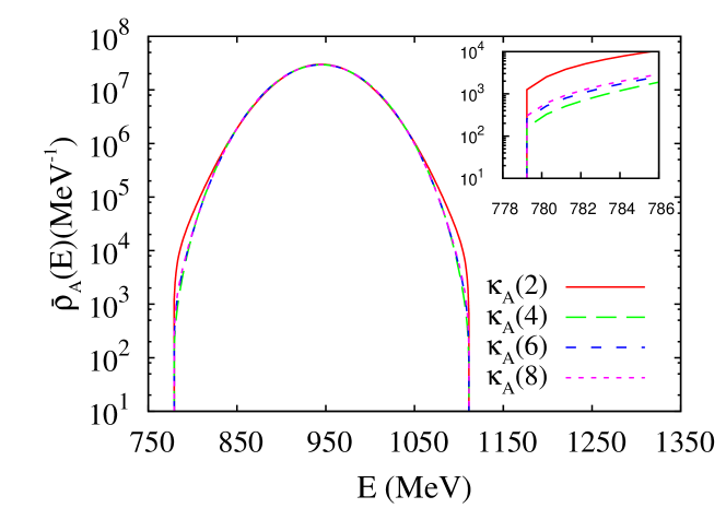
Figure 1: Level density $\overline{\rho}_{A}(E)$ as a function of energy $E$ for the case of $\overline{\rho}^{(0)}_{1}$ and for parameter values given in the text. The cumulant sum of the Fourier transform (23) includes the terms up to the listed cumulant $\kappa_{A}$. The inset shows $\overline{\rho}_{A}(E)$ in the tails.

We compare results for the continuous single-particle level density given by the first of Eqs. (41) with those of Ref. [4] where a sum of delta functions was used. In Ref. [4], the level density $\overline{\rho}_{A}(E)$ is calculated exactly for sufficiently small values for $B$ and $A$ and, in addition, is approximated by fitting the expression $\overline{\rho}_{A}(E)\propto\exp\{-\gamma_{2}(E)^{2}-\gamma_{4}(E)^{4}-\gamma_{6}(E)^{6}\}$ to the first three moments $M_{A}(2)$, $M_{A}(4)$, $M_{A}(6)$. For the comparison we consider for both exact and fitted results [4] the constant spacing $d=V/B^{(0)}=0.88$ MeV. We use the first four non-vanishing cumulants $\kappa_{A}(2)$, $\kappa_{A}(4)$, $\kappa_{A}(6)$ and $\kappa_{A}(8)$ for the Fourier transform in Eq. (23) and $n=30$ orthogonal polynomials. In the present case, the spectrum extends from $(d/2)A^{2}$ to $d[B^{(0)}A-(1/2)A^{2}]$ while in the case of Ref. [4] it extends from $(d/2)A(A+1)$ to $d[B^{(0)}A-(1/2)A(A-1)]$. We have taken account of this difference by shifting the spectrum calculated in the present framework by $+(d/2)A$. For the same set of parameters as in Fig. 1, Fig. 2 shows the exact values for the level density $\overline{\rho}_{A}(E)$ (solid red line), the approximation of Ref. [4] based upon a fit using up to the sixth moment (long dashed green line), and the approximation using up to the eighth cumulant and the expansion in terms of orthogonal polynomials (short dashed blue line, shifted). We see that both approximate methods, while very good near the center of the spectrum, fail near the boundaries where $\overline{\rho}_{A}(E)=1$. By construction, the method of orthogonal polynomials yields $\overline{\rho}_{A}(E)=0$ at the minimum and maximum energies $E_{1}$ and $E_{N}$ of the spectrum. Close to the spectrum tails, however, the spectrum is broader than the exact results and overestimates the exact values somewhat more than the fitting procedure of Ref. [4].

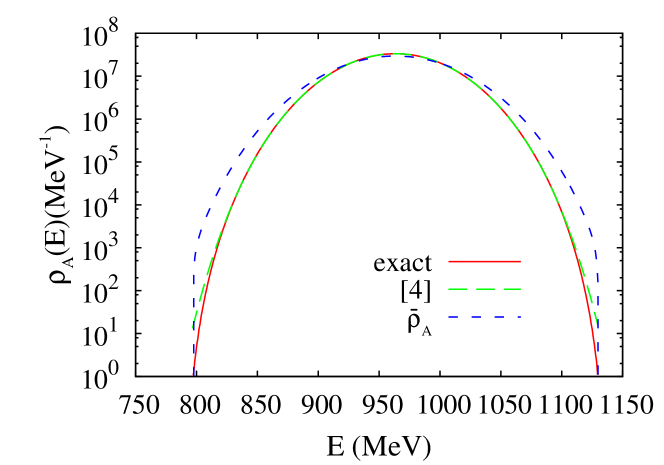
Figure 2: Comparison of our present results for the continuous single-particle level density $\overline{\rho}_{1}^{(0)}$ using cumulants up to $\kappa_{A}(8)$ (short dashed blue line) with the exact level density $\rho_{A}(E)$ (red solid line) and results of the fitting procedure described in Ref. [4] (long dashed green line) for $A=42$ and $B^{(0)}=51$. For a better visualization the level density $\overline{\rho}_{A}$ is shifted by $(d/2)A=18$ MeV towards higher energies.

Compared to Ref. [4], the strength of our method is that we can go beyond the constant-spacing model. For medium-weight (heavy) nuclei, we use the linear (quadratic) single-particle level density $\overline{\rho}^{(1)}_{1}(\varepsilon)$ ($\overline{\rho}^{(2)}_{1}(\varepsilon)$) of Eq. (41), respectively. Here the odd moments and cumulants of the distribution also come into play, and the many-body density is no longer symmetric about its center. For $\overline{\rho}^{(1)}_{1}(\varepsilon)$, Fig. 3 shows the normalized level density $\overline{R}_{A}(E)$ as a function of energy $E$ for $A=100$ and $B^{(1)}=148$ and two different cutoffs in the Fourier transform sum (23). The Fermi energy and the range of the single-particle spectrum are $F=37$ MeV and $V=45$ MeV, respectively. The many-body spectrum extends from $E_{1}=$2466 MeV to $E_{N}=$3620 MeV. We find that for these parameters the use of $n=50$ orthogonal polynomials is sufficient; no noticeable changes occur as $n$ is increased further. For the level density calculated using cumulants up to $\kappa_{A}(4)$ in Eq. (23) there exist intervals in the tails of the spectrum where $\overline{R}_{A}(E)$ becomes negative (and is therefore not displayed on the logarithmic scale), while using cumulants up to $\kappa_{A}(6)$ in Eq. (23) yields strictly positive values.

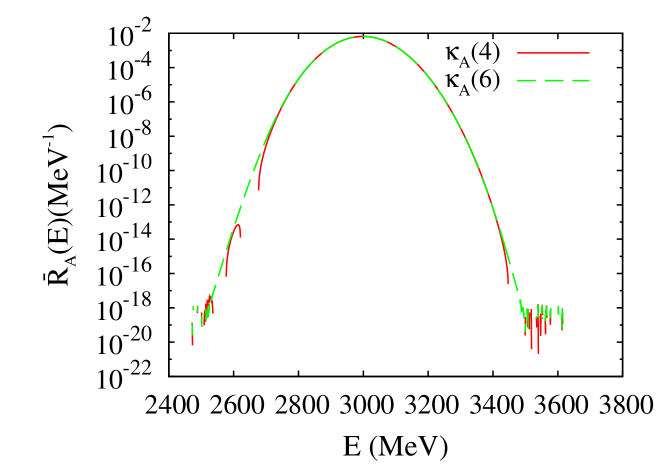
Figure 3: Normalized level density $\overline{R}_{A}(E)$ as a function of energy $E$ for $\overline{\rho}^{(1)}_{1}(\varepsilon)$ and $A=100$ and $B^{(1)}=148$. The Fourier transform is calculated according to Eq. (23) using the cumulants of Eqs. (24) up to $\kappa_{A}(4)$ (red solid line) and $\kappa_{A}(6)$ (green dashed line).

In Fig. 4 we compare our result using $\overline{\rho}^{(1)}_{1}$ and cumulants up to $\kappa_{A}(6)$ with the normalized level density for the constant-spacing model calculated as described in Ref. [4], with single-particle level spacing $d=V/B^{(1)}$ and $V=45$ MeV. The latter method yields values for the level density $\overline{R}_{A}(E)$ throughout the spectrum but overestimates $\overline{R}_{A}(E)$ in the tails while our present result does not cover values of $\overline{R}_{A}(E)$ that are smaller than $10^{-21}$ times the maximum. We note three significant differences between the results for the constant-spacing model and for $\overline{\rho}^{(1)}_{1}$. (i) The spectrum is shifted by 700 MeV towards higher energies. However, part of this shift is due to an increase of the ground-state energy. (ii) The width of the many-body level density is smaller for $\overline{\rho}^{(1)}_{1}$ than for the constant-spacing model. (iii) For $\overline{\rho}^{(1)}_{1}$ (and also for $\overline{\rho}^{(2)}_{1}$), the odd cumulants $\kappa_{A}(3)<0$ and $\kappa_{A}(5)<0$ cause an asymmetry in the many-body level density. Therefore, the maximum of $\overline{R}_{A}(E)$ is below the center of the spectrum in both cases. For $\overline{\rho}^{(1)}_{1}$ it occurs at $3000$ MeV while the center is at $E_{c}=3043$ MeV. The temperature of the system, defined in terms of the inverse of the derivative of $\overline{\rho}_{A}(E)$, becomes infinite at the maximum. This is consistent with the Fermi-gas model of Eqs. (3) to (7) where infinite temperature (defined by $\beta=0$) is attained at the mean energy $E_{0}=3000$ MeV of the system.

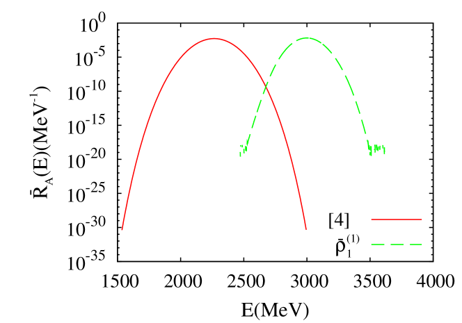
Figure 4: The normalized level density $\overline{R}_{A}(E)$ for $\overline{\rho}^{(1)}_{1}$ and $A=100$, $B^{(1)}=148$ considering cumulants up to $\kappa_{A}(6)$ (green dashed line) compared to the result of the constant-spacing model with single-particle level spacing $d=V/B^{(1)}$ using the fitting procedure described in Ref. [4] (full red line).

For the case of $\overline{\rho}^{(2)}_{1}$ we consider $A=200$, $B^{(2)}=360$, $V=45$ MeV and $F=37$ MeV and calculate the normalized level density $\overline{R}_{A}(E)$ taking into account the cumulants in Eqs. (24) up to $\kappa_{A}(6)$. The number of orthogonal polynomials used for the calculation is $n=100$. The ratio $\overline{\rho}_{A}(E)/\overline{R}_{A}(E)\approx 10^{106}$ is huge. A comparison with the density for constant single-particle level spacing $d=V/B^{(2)}$ calculated as in Ref. [4] is displayed in Fig. 5 and shows the same features as seen for $\overline{\rho}^{(1)}_{1}$: the distribution is shifted towards higher energies, is more narrow, and is asymmetric. As for $\overline{\rho}^{(1)}_{1}$, our approximation covers roughly the leading $20$ orders of magnitude of the distribution.

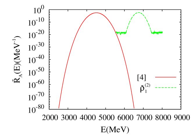
Figure 5: The normalized level density $\overline{R}_{A}(E)$ for $\overline{\rho}^{(2)}_{1}$ and $A=200$, $B^{(2)}=360$ considering cumulants up to $\kappa_{A}(6)$ (dashed green line) compared to results of the constant-spacing model with single-particle level spacing $d=V/B^{(2)}$ using the method described in Ref. [4] (solid red line).

4 Asymptotic Expansion

The results in Section 3 are obtained by using only the lowest cumulants in the Fourier transform of Eq. (23). The omission of higher-order cumulants can be justified asymptotically, i.e., for $B\gg 1$ and $A\gg 1$. (Here and in what follows $B,A\gg 1$ means $A\approx B/2\gg 1$. Because of particle-hole symmetry, the asymptotic approximation fails not only as $A$ approaches $1$ from above but also as $A$ approaches $B$ from below). In Ref. [4] we have shown for the constant-spacing model that in the asymptotic regime the contributions to the sum over $k$ in Eq. (21) decrease very rapidly with increasing $k$. In D we extent this proof to the two other cases in Eqs. (41). In both these cases, too, the rescaled cumulants decrease very rapidly with increasing $k$. As a by-product we find that the resulting asymptotic expression for the Fourier transform in Eq. (23) becomes much simpler than the full expression.

We emphasize that the asymptotic behavior of the rescaled cumulants obtained in Eqs. (79) is generic. Indeed, this behavior is due to the fact that the unscaled cumulants are all proportional to $A$. This fact, in turn, is due to the normalization condition (34). For an arbitrary single-particle level density $\omega_{1}(\varepsilon)$ that same condition yields for the normalized form $\overline{\rho}_{1}(E)=A\omega_{1}(\varepsilon)/\int_{0}^{F}{\rm d}\varepsilon^{\prime}\omega(\varepsilon^{\prime})$. The moments of single-particle energies in Eqs. (71) can generally be written as $\sum_{j}(\varepsilon_{j})^{k}=\int_{0}^{V}{\rm d}\varepsilon\ \overline{\rho}_{1}(\varepsilon)\varepsilon^{k}$. Thus, all these moments and the corresponding cumulants are proportional to $A$. This implies the asymptotic form (79). The constants multiplying $A^{-k/2}$ depend on the form of $\omega(\varepsilon)$. We expect that these constants are of order unity for any function $\omega(\varepsilon)$ that distributes the single-particle energies $\varepsilon_{j}$ more or less uniformly over the interval $\{0,V\}$.

4.1 Examples

For a comparison of the asymptotic with the full results we need the asymptotic values of the cumulants. Eq. (42) gives $A/B=F^{2}/V^{2}$ ($A/B=F^{3}/V^{3}$) for $\rho^{(1)}_{1}$ ($\rho^{(2)}_{1}$, respectively). We use Eqs. (73) and (18) and define $f_{1}=F^{2}/V^{2}$ and $f_{2}=F^{3}/V^{3}$. For the case of $\rho_{A}^{(1)}(E)$ we obtain

$$\kappa^{(1)}_{A}(2) = \frac{1}{18}AV^{2}(1-f_{1})\ ,$$

$$\kappa^{(1)}_{A}(3) = -\frac{1}{135}AV^{3}(1-f_{1})(1-2f_{1})\ ,$$

$$\kappa^{(1)}_{A}(4) = \frac{1}{135}AV^{4}(1-f_{1})(1-6f_{1}+6f^{2}_{1}),$$

$$\kappa^{(1)}_{A}(5) = -\frac{4}{1701}AV^{5}(1-f_{1})(1-14f_{1}+36f^{2}_{1}-24f^{3}_{1})\ ,$$

$$\kappa^{(1)}_{A}(6) = \frac{31}{20412}AV^{6}(1-f_{1})(1-30f_{1}+150f^{2}_{1}-240f^{3}_{1}+120f^{4}_{1})\ ,$$ (44)

and for the case of $\rho_{A}^{(2)}(E)$,

$$\kappa^{(2)}_{A}(2) = \frac{3}{80}AV^{2}(1-f_{2})\ ,$$

$$\kappa^{(2)}_{A}(3) = -\frac{1}{160}AV^{3}(1-f_{2})(1-2f_{2})\ ,$$

$$\kappa^{(2)}_{A}(4) = \frac{39}{8960}AV^{4}(1-f_{2})(1-6f_{2}+6f^{2}_{2})\ ,$$

$$\kappa^{(2)}_{A}(5) = -\frac{3}{1792}AV^{5}(1-f_{2})(1-14f_{2}+36f^{2}_{2}-24f^{3}_{2})\ ,\$$

$$\kappa^{(2)}_{A}(6) = \frac{79}{86016}AV^{6}(1-f_{2})(1-30f_{2}+150f^{2}_{2}-240f^{3}_{2}+120f^{4}_{2})\ .$$ (45)

The comparison of the level density calculated with the exact cumulants up to $\kappa_{A}(6)$ as in Section 3 and the asymptotic ones shows that the agreement is very good and improves with increasing values of particle number $A$ and level number $B$. As an example we show in Fig. 6 results for $\overline{\rho}_{1}^{(1)}(E)$ with $V=45$ MeV, $F=37$ MeV and $A=100$, $B=148$. We note the slightly larger asymmetry in the low-energy part of the spectrum calculated with the asymptotic values. Furthermore, an energy interval with unphysical negative level density appears around 3400 MeV in the high-energy part of the spectrum. A similar comparison for $\overline{\rho}_{1}^{(2)}(E)$ with the same parameters $V$, $F$ and particle and level numbers $A=200$ and $B=360$, respectively, is shown in Fig. 7. In this case the results for the exact and the asymptotic values for the cumulants are almost indistinguishable; the slightly more pronounced asymmetry of the asymptotic results is barely visible.

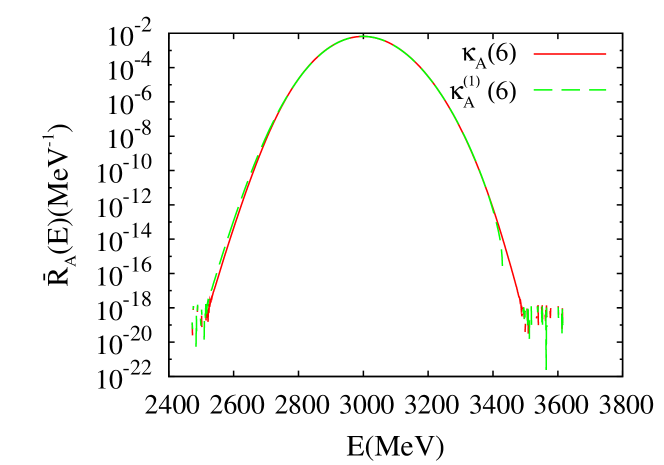
Figure 6: The normalized level density $\overline{R}_{A}(E)$ for $\overline{\rho}_{1}^{(1)}(E)$ and $A=100$, $B^{(1)}=148$ using the first six exact (red solid line) and asymptotic (green dashed line) cumulants. The number of orthogonal polynomials used for the calculation is $n=50$.

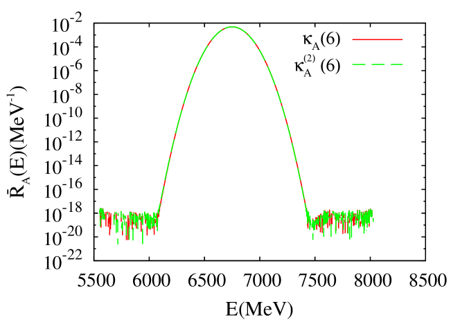
Figure 7: The normalized level density $\overline{R}_{A}(E)$ for $\overline{\rho}_{1}^{(2)}(E)$ and $A=200$, $B^{(2)}=360$ using the first six exact (red solid line) and asymptotic (green dashed line) cumulants. The number of orthogonal polynomials used for the calculation is $n=100$.

5 Density of Particle-Hole States

To calculate pre-equilibrium processes, the densities of $p$-particle $p$-hole states are needed in addition to the total level density worked out in the previous Sections. A $p$-particle $p$-hole state has $p$ particles above the Fermi energy $F$ and $(A-p)$ particles below $F$. We now show that these densities are easily obtained by adapting the formulas obtained previously.

For the hole states there are $(A-p)$ particles distributed over the $A$ single-particle states in the energy interval $\{0,F\}$. We work with these $(A-p)$ particles (instead of the $p$ holes) throughout but use the terminology of “hole states”. The Fermi energy $F_{h}$ of the $(A-p)$ particles is defined by the analogue of Eq. (33) as

$$A-p=\int_{0}^{F_{h}}{\rm d}\varepsilon\ \overline{\rho}_{1}(\varepsilon)\ .$$ (46)

The results in Eqs. (56) and (71) for the low moments and in Eqs. (44), (45) for the asymptotic cumulants are transcribed to the case of hole states by the replacements $B\to A,A\to(A-p),V\to F,F\to F_{h}$. With $i=1,2$ this yields the full or the asymptotic expressions for the Fourier transforms ${\cal F}^{(i)}_{A-p}(\tau)$ of the densities $R^{(i)}_{A-p}(E)$. These are normalized to unity. The full densities are given by $\rho^{(i)}_{A-p}(E)=N^{(i)}_{A-p}R^{(i)}_{A-p}(E)$, with $N^{(i)}_{A-p}={A\choose A-p}=S^{(i)}$. The spectrum extends from $E^{(i)}_{1,A-p}$ to $E^{(i)}_{{S^{(i)}},A-p}$ and has mean energy $E^{(i)}_{0,A-p}$. These energies are defined in analogy to Eqs. (43).

For the particle states there are $p$ particles distributed over the $(B^{(i)}-A)$ single-particle states in the energy interval $\{F,V\}$. The Fermi energy is defined by

$$p=\int_{F}^{F_{p}}{\rm d}\varepsilon\ \overline{\rho}_{1}(\varepsilon)\ .$$ (47)

The sums $\sum_{j}(\tilde{\varepsilon}_{j})^{k}$ are conveniently determined as the differences between the total sums given in Eqs. (71) and the sums for the hole states as determined in the previous paragraph. The transcriptions $B\to(B^{(i)}-A),A\to p$ and Eqs. (56) yield the low moments. For the asymptotic cumulants, we also replace $V\to(V-F)$ and $F\to F_{p}$. This yields the full or the asymptotic forms of the Fourier transforms ${\cal F}^{(i)}_{p}(\tau)$ of the normalized densities $R^{(i)}_{p}(E)$. The full densities are given by $\rho^{(i)}_{p}(E)=N^{(i)}_{p}R^{(i)}_{p}(E)$, with $N^{(i)}_{p}={B^{(i)}-A\choose p}=T^{(i)}$. The spectrum extends from $E^{(i)}_{1,p}$ to $E^{(i)}_{{T^{(i)}},p}$ and has mean energy $E^{(i)}_{0,p}$. These energies are defined in analogy to Eqs. (43).

The level density $\rho_{A-p,p}(E)=N^{(i)}_{A-p}N^{(i)}_{p}R_{A-p,p}(E)$ for the $p$-particle $p$-hole states is the convolution of $\rho_{A-p}(E)$ and of $\rho_{p}(E)$. We replace all densities $\rho$ by the normalized densities $R$ and Fourier transform the result. Then the Fourier transform ${\cal F}^{(i)}_{A-p,p}(E)$ of $R_{A-p,p}(E)$ is given by

$${\cal F}^{(i)}_{A-p,p}(\tau) = \int_{-\infty}^{+\infty}{\rm d}E\ \exp\{i(E-E_{0,p}-E_{0,A-p})\tau\}\int_{-\infty}^{+\infty}{\rm d}E_{1}\int_{-\infty}^{+\infty}{\rm d}E_{2}$$ (48)

$$\qquad\qquad\times\delta(E-E_{1}-E_{2})\rho^{(i)}_{A-p}(E_{1})\rho^{(i)}_{p}(E_{2})$$

$$= {\cal F}^{(i)}_{A-p}(\tau){\cal F}^{(i)}_{p}(\tau)\ .$$

The spectrum extends from $E^{(i)}_{1,A-p}+E^{(i)}_{1,p}$ to $E^{(i)}_{{S^{(i)}},A-p}+E^{(i)}_{{T^{(i)}},p}$. In this interval the expression (48) can be used straightforwardly for an expansion in orthogonal polynomials. It is gratifying to see that the calculation of the particle-hole density requires only about the same effort as the calculation of the total density.

6 Density of Accessible States and of Accessible Particle-Hole States

The density $\rho_{\rm acc}(E)$ of accessible states is an important concept in the theory of pre-equilibrium reactions. It is used to determine the rate for transitions induced by an external agent (an impinging proton, or a laser photon, for instance). Here we define $\rho_{\rm acc}(E)$ for processes where an external agent (a laser pulse, for example) excites an individual nucleon from a many-body state at energy $E$ to another such state at energy $E+\Delta E$. We assume that at both energies the nucleus is in thermal equilibrium and calculate $\rho_{\rm acc}(E)$ in the framework of the Fermi-gas model of Eqs. (37) and (38). At high excitation energies this model is much simpler to use than the usual counting procedure for $\rho_{\rm acc}(E)$.

With $n_{A,E}(\varepsilon)$ the probability of finding a single-particle state with energy $\varepsilon$ occupied when the nucleus has total energy $E$ and $(1-n_{A,E+\Delta}(\varepsilon+\Delta))$ the probability of finding a single-particle state with energy $\varepsilon+\Delta$ empty when the nucleus has total energy $E+\Delta$, the number ${\cal N}_{\rm acc}(E,\Delta)$ of accessible states is given by the product of both probabilities, integrated over all $\varepsilon$ obeying $0\leq\varepsilon\leq V-\Delta$,

$${\cal N}_{\rm acc}(E,\Delta)=\int_{0}^{V-\Delta}{\rm d}\varepsilon\ n_{A,E}(\varepsilon)(1-n_{A,E+\Delta}(\varepsilon+\Delta))\overline{\rho}_{1}(\varepsilon)\ .$$ (49)

The density of accessible states is obtained by weighing the integrand with the single-particle level density at energy $\varepsilon+\Delta$,

$$\rho_{\rm acc}(E,\Delta)=\int_{0}^{V-\Delta}{\rm d}\varepsilon\ n_{A,E}(\varepsilon)(1-n_{A,E+\Delta}(\varepsilon+\Delta))\overline{\rho}_{1}(\varepsilon)\overline{\rho}_{1}(\varepsilon+\Delta)\ .$$ (50)

The range of $\Delta$ is $0\leq\Delta\leq V$. Densities of accessible states for the three cases of single-particle level densities defined in Eqs. (41) are shown in Fig. 8. Obviously, the stronger the increase of $\overline{\rho}_{1}(\varepsilon)$ with single-particle energy $\varepsilon$, the bigger the density of accessible states. Conversely, increasing the energy $E$ of the many–body system makes $n_{A,E}(\varepsilon)$ (which is a step-like function of $\varepsilon$ at low energies) an ever more smooth function of $\varepsilon$. At infinite temperature, $n_{A,E}(\varepsilon)$ is a constant independent of $\varepsilon$. These facts cause $\rho_{\rm acc}(E,\Delta)$ to decrease strongly with increasing $E$.

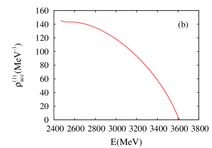
Figure 8: Density of accessible states $\rho_{\rm acc}(E,\Delta)$ for $\Delta=5$ MeV and single-particle level densities (a) $\overline{\rho}_{1}^{(0)}$, (b) $\overline{\rho}_{1}^{(1)}$ and (c) $\overline{\rho}_{1}^{(2)}$ for the same parameters as used in Section 3.

In pre-equilibrium models, the rates for transitions at fixed energy $E$ between states carrying different particle-hole numbers determine the rate of equilibration of the compound nucleus. The transition rates are proportional to the density of accessible states. We generalize the Fermi-gas model of Eqs. (37) and (38) to the case where particle number $p$ and hole number $p$ are fixed, see Section 5. We then deal with two gases in thermal equilibrium,

$$n_{A-p,E}(\varepsilon)=\frac{\Theta(F-\varepsilon)}{1+\exp\{\beta\varepsilon+\alpha_{A-p}\}}\ ,\ n_{p,E}(\varepsilon)=\frac{\Theta(\varepsilon-F)}{1+\exp\{\beta\varepsilon+\alpha_{p}\}}\ .$$ (51)

Here $\Theta$ is the Heaviside function. The constants $\beta,\alpha_{p}$ and $\alpha_{A-p}$ are determined by the constraints

$$A-p = \int_{0}^{F}{\rm d}\varepsilon\ n_{A-p,E}(\varepsilon)\overline{\rho}_{1}(\varepsilon)\ ,$$

$$p = \int_{F}^{V}{\rm d}\varepsilon\ n_{p,E}(\varepsilon)\overline{\rho}_{1}(\varepsilon)\ ,$$

$$E = \int_{0}^{V}{\rm d}\varepsilon\ \varepsilon(n_{p,E}(\varepsilon)+n_{A-p}(\varepsilon))\overline{\rho}_{1}(\varepsilon)\ .$$ (52)

The process leading from a $p$-particle $p$-hole state to a $(p+1)$-particle $(p+1)$-hole state at the same energy $E$ consists in lifting a particle from a single-particle state at energy $\varepsilon_{1}$ below the Fermi energy $F$ to a state at energy $(\varepsilon_{1}+\Delta)$ above $F$. The required energy $\Delta$ is either taken from a particle at energy $\varepsilon_{2}>F$ that is moved to a state at energy $\varepsilon_{2}-\Delta>F$, or from a particle at energy $\varepsilon_{3}<F$ that is moved to a state at energy $(\varepsilon_{3}-\Delta)$. For clarity we define

$$\overline{\rho}_{1,<}(\varepsilon)=\Theta(F-\varepsilon)\overline{\rho}_{1}(\varepsilon)\ ,\ \overline{\rho}_{1,>}(\varepsilon)=\Theta(\varepsilon-F)\overline{\rho}_{1}(\varepsilon)\ .$$ (53)

We recall that $\overline{\rho}_{1}(\varepsilon)=0$ for $\varepsilon<0$ and for $\varepsilon>V$. According to Eq. (50), the densities of accessible states for the three processes are

$$\rho_{{\rm acc},1}(E,\Delta) = \int_{-\infty}^{\infty}{\rm d}\varepsilon_{1}\ n_{A-p,E}(\varepsilon_{1})(1-n_{p,E}(\varepsilon_{1}+\Delta))$$

$$\qquad\times\overline{\rho}_{1,<}(\varepsilon_{1})\overline{\rho}_{1,>}(\varepsilon_{1}+\Delta)\ ,$$

$$\rho_{{\rm acc},2}(E,\Delta) = \int_{-\infty}^{\infty}{\rm d}\varepsilon_{2}\ n_{p,E}(\varepsilon_{2})(1-n_{p,E}(\varepsilon_{2}-\Delta))\overline{\rho}_{1,>}(\varepsilon_{2})\overline{\rho}_{1,>}(\varepsilon_{2}-\Delta)\ ,$$

$$\rho_{{\rm acc},3}(E,\Delta) = \int_{-\infty}^{\infty}{\rm d}\varepsilon_{3}\ n_{p,E}(\varepsilon_{3})(1-n_{p,E}(\varepsilon_{3}-\Delta))\overline{\rho}_{1,<}(\varepsilon_{3})\overline{\rho}_{1,<}(\varepsilon_{3}-\Delta)\ .$$

(54)

Because of the definitions (53), we need not restrict the ranges of integration in Eqs. (54) or the range of $\Delta$. The density of accessible $(p+1)$-particle $(p+1)$-hole states is given by

$$\rho_{\rm acc}(E) = \frac{1}{2}\int_{-\infty}^{\infty}\ {\rm d}\Delta\ \rho_{{\rm acc},1}(E,\Delta)\rho_{{\rm acc},2}(E,\Delta)$$ (55)

$$\qquad+\frac{1}{2}\int_{-\infty}^{\infty}{\rm d}\Delta\ \rho_{{\rm acc},1}(E,\Delta)\rho_{{\rm acc},3}(E,\Delta)\ .$$

The substitution $\Delta\to(\varepsilon_{2}-\varepsilon_{1}-\Delta^{\prime})$ shows that the two indistinguishable processes $\varepsilon_{1}\to(\varepsilon_{1}+\Delta)$, $\varepsilon_{2}\to(\varepsilon_{2}-\Delta)$ and $\varepsilon_{1}\to(\varepsilon_{2}-\Delta)$, $\varepsilon_{2}\to(\varepsilon_{1}+\Delta)$ are both contained in the first integral. To avoid double counting we introduce the factor $1/2$. The same argument applies to the processes $\varepsilon_{1}\to(\varepsilon_{1}+\Delta)$, $\varepsilon_{3}\to(\varepsilon_{3}-\Delta)$ and $\varepsilon_{3}\to(\varepsilon_{1}+\Delta)$, $\varepsilon_{1}\to(\varepsilon_{3}-\Delta)$, hence the second factor $1/2$.

7 Summary and Conclusions

The level density is a basic property of atomic nuclei. It has been the object of theoretical and experimental investigations since the beginnings of nuclear physics. In the present work we have focused attention on the domain of high excitation energies (several $100$ MeV above yrast) and large particle numbers ($A\geq 100$). For the theoretical description of heavy-ion reactions at several MeV per nucleon and of reactions induced by coherent laser beams with several MeV per photon, one needs to know the level density $\rho_{A}(E)$ in that domain where (measured in units of the mean single-particle density) $\rho_{A}(E)$ easily attains values of $10^{40}$ or $10^{50}$.

Starting from a set of single-particle energies given either empirically or in terms of a mean-field approximation and generalizing the approach developed in Ref. [4], we have have written $\rho_{A}(E)$ as the sum of all ways of distributing $A$ spinless Fermions over the available single-particle states. We have derived an exact closed-form expression for the Fourier transform (with respect to energy $E$) and Laplace transform (with respect to particle number $A$) of $\rho_{A}(E)$. That expression yields exact values for the lowest moments and for the lowest cumulants of $\rho_{A}(E)$. These depend on binomial coefficients and on the moments of the single-particle energies. They were used to construct approximate expressions for the Fourier transform of $\rho_{A}(E)$ and, from there, approximate expressions for the coefficients of an expansion of $\rho_{A}(E)$ in terms of orthogonal polynomials. As an alternative to using a fixed set of single-particle energies we have also considered a smooth form of the single-particle level density $\overline{\rho}_{1}(\varepsilon)$. We have demonstrated that the approach converges: For $A\gg 1$ and realistic forms of $\overline{\rho}_{1}(\varepsilon)$, the cumulants $\kappa_{A}(k)$ quickly decrease with increasing $k$. We have shown that the huge values of the level density attained at the center of the spectrum make it appear very unlikely that a uniform approximation to $\rho_{A}(E)$ (valid throughout the spectrum) will ever be practicable. In that sense, our approach complements the standard approaches to calculating $\rho_{A}(E)$ that focus on low excitation energies and small particle numbers. Being entirely analytical, the present approach provides direct insight into the overall dependence of $\rho_{A}(E)$ on energy. Moreover, it is easy to implement.

For the constant-spacing model we have tested our approach against exact numerical results from Ref. [4], and we have compared it with approximate results of Ref. [4] where the low moments of $\rho_{A}(E)$ were used as fit parameters. We find good agreement in the center of the spectrum whereas our results give too high values for $\rho_{A}(E)$ in the tails. The present approach is not confined to the (unrealistic) constant-spacing model, and we have calculated $\rho_{A}(E)$ using two more realistic energy-dependent forms of $\overline{\rho}_{1}(\varepsilon)$. (The approach can easily be used for other forms). As in the case of the constant-spacing model, our approach fails in the tails of $\rho_{A}(E)$. We have shown that as the dependence of $\overline{\rho}_{1}(\varepsilon)$ on the single-particle energy $\varepsilon$ increases, the maximum of $\rho_{A}(E)$ is significantly shifted toward higher excitation energy, the spectrum becomes asymmetric, and the width in energy of $\rho_{A}(E)$ decreases. For large particle numbers our approximation covers about half the spectrum around the center and a range of values of $\rho_{A}(E)$ covering about 20 orders of magnitude.

Using the same technique we have also determined particle-hole densities in the domain of large excitation energies and particle numbers. The calculation of these quantities is as straightforward as that of $\rho_{A}(E)$. It goes without saying that instead of considering Fermions, we can use our approach also to determine level densities in cases where neutrons and protons are considered separate entities. For the calculation of the density $\rho_{\rm acc}$ of accessible states we have used an equilibrated Fermi-gas model and several forms of $\overline{\rho}_{1}(\varepsilon)$. Our results are intuitively obvious: $\rho_{\rm acc}$ increases strongly with increasing energy dependence of $\overline{\rho}_{1}(\varepsilon)$, and it decreases strongly with increasing excitation energy.

The present approach is limited to non-interacting Fermions. The nucleon-nucleon interaction can be partially taken into account in terms of a mean-field approach. Even the results of a temperature-dependent Hartree-Fock approximation can be accommodated by readjusting the cumulants for each value of the temperature. Thus, we expect the method will be useful for a broad range of applications.

Appendix A Moments of the Density

Combining Eqs. (21), (19), and (15) we obtain [4] for $k=0,1,\ldots,6$

$$m_{A}(0) = {B\choose A}\ ,$$

$$m_{A}(1) = 0\ ,$$

$$m_{A}(2) = {B-2\choose A-1}\ \sum_{j=1}^{B}(\tilde{\varepsilon}_{j})^{2}\ ,$$

$$m_{A}(3) = \bigg{\{}{B-3\choose A-1}-{B-3\choose A-2}\bigg{\}}\ \sum_{j=1}^{B}(\tilde{\varepsilon}_{j})^{3}\ ,$$

$$m_{A}(4) = \bigg{\{}{B-4\choose A-1}-4{B-4\choose A-2}+{B-4\choose A-3}\bigg{\}}\ \sum_{j=1}^{B}(\tilde{\varepsilon}_{j})^{4}$$

$$+3{B-4\choose A-2}\ \bigg{(}\sum_{j=1}^{B}(\tilde{\varepsilon}_{j})^{2}\bigg{)}^{2}\ ,$$

$$m_{A}(5) = \bigg{\{}{B-5\choose A-1}-11{B-5\choose A-2}+11{B-5\choose A-3}-{B-5\choose A-4}\bigg{\}}\ \sum_{j=1}^{B}(\tilde{\varepsilon}_{j})^{5}$$

$$+10\bigg{\{}{B-5\choose A-2}-{B-5\choose A-3}\bigg{\}}\ \sum_{j=1}^{B}(\tilde{\varepsilon}_{j})^{2}\sum_{j=1}^{B}(\tilde{\varepsilon}_{j})^{3}\ ,$$

$$m_{A}(6) = \bigg{\{}{B-6\choose A-1}-26{B-6\choose A-2}+66{B-6\choose A-3}-26{B-6\choose A-4}$$

$$\qquad\qquad+{B-6\choose A-5}\bigg{\}}\ \sum_{j=1}^{B}(\tilde{\varepsilon}_{j})^{6}$$

$$+15\bigg{\{}{B-6\choose A-2}-4{B-6\choose A-3}+{B-6\choose A-4}\bigg{\}}\ \sum_{j=1}^{B}(\tilde{\varepsilon}_{j})^{2}\sum_{j=1}^{B}(\tilde{\varepsilon}_{j})^{4}$$

$$+10\bigg{\{}{B-6\choose A-2}-2{B-6\choose A-3}+{B-6\choose A-4}\bigg{\}}\ \bigg{(}\sum_{j=1}^{B}(\tilde{\varepsilon}_{j})^{3}\bigg{)}^{2}$$

$$+15{B-6\choose A-3}\ \bigg{(}\sum_{j=1}^{B}(\tilde{\varepsilon}_{j})^{2}\bigg{)}^{3}\ .$$

For the single-particle model with constant level density we extend the calculation to $k=8$. In that case we have $m_{A}(7)=0$ and

$$m_{A}(8) = \ \sum_{j=1}^{B}(\tilde{\varepsilon}_{j})^{8}\ \bigg{\{}{B-8\choose A-1}-120{B-8\choose A-2}+1191{B-8\choose A-3}$$ (56)

$$-2416{B-8\choose A-4}+1191{B-8\choose A-5}-120{B-8\choose A-6}$$

$$\qquad+{B-8\choose A-7}\bigg{\}}$$

$$+28\ \sum_{j=1}^{B}(\tilde{\varepsilon}_{j})^{2}\ \sum_{j=1}^{B}(\tilde{\varepsilon}_{j})^{6}\ \bigg{\{}{B-8\choose A-2}-26{B-8\choose A-3}+66{B-8\choose A-4}$$

$$\qquad-26{B-8\choose A-5}+{B-8\choose A-6}\bigg{\}}$$

$$+35\ \bigg{(}\sum_{j=1}^{B}(\tilde{\varepsilon}_{j})^{4}\bigg{)}^{2}\ \bigg{\{}{B-8\choose A-2}-8{B-8\choose A-3}+18{B-8\choose A-4}$$

$$\qquad-8{B-8\choose A-5}+{B-8\choose A-6}\bigg{\}}$$

$$+210\ \bigg{(}\sum_{j=1}^{B}(\tilde{\varepsilon}_{j})^{2}\bigg{)}^{2}\ \sum_{j=1}^{B}(\tilde{\varepsilon}_{j})^{4}\ \bigg{\{}{B-8\choose A-3}-4{B-8\choose A-4}$$

$$\qquad+{B-8\choose A-5}\bigg{\}}$$

$$+105\ \bigg{(}\sum_{j=1}^{B}(\tilde{\varepsilon}_{j})^{2}\bigg{)}^{4}\ {B-8\choose A-4}\ .$$

Appendix B In Search of a Uniform Approximation to $\rho_{A}(E)$

To justify our claim that different approximations are needed in different parts of the spectrum, we use as a model the smooth equivalent of the constant-spacing model, i.e, a smooth single-particle level density $\overline{\rho}_{1}(E)=1/d$ for $-V/2\leq E\leq V/2$ and $\overline{\rho}_{1}(E)=0$ otherwise. It is clear from the outset and shown presently that we cannot hope for exact agreement with results obtained for a level density of the form $\rho_{1}(E)=\sum_{j}\delta(E-dj)$. That is irrelevant, however, for our claim. For the many-body level density $\rho_{A}(E)$ we use the ansatz

$$\rho_{A}(E) = \frac{1}{d^{A}}\frac{1}{A!}\int_{-V/2}^{V/2}{\rm d}E_{1}\int_{-(V-d)/2}^{(V-d)/2}{\rm d}E_{2}\times\ldots\times\int_{-(V-(A-1)d)/2}^{(V-(A-1)d)/2}{\rm d}E_{A}$$ (57)

$$\times\delta(E_{1}+E_{2}+\ldots E_{A}-E)\ .$$

The factor $1/A!$ takes care of the exclusion principle. The limits of integration are chosen in such a way as to be consistent with both the domain of definition of $\overline{\rho}_{1}(E)$ and the fact that the level density vanishes for $V\leq dA$. As we shall see, this choice also guarantees the correct normalization of $\rho_{A}(E)$. The price we have to pay is that the range of $\rho_{A}(E)$ is not reproduced correctly. For the constant-spacing model that range (after a suitable shift of energy) is given [4] by $-(1/2)VA+(1/2)dA^{2}\leq E\leq(1/2)VA-(1/2)dA^{2}$ while Eq. (57) implies $-(1/2)VA+(1/4)dA(A-1)\leq E\leq(1/2)VA-(1/4)dA(A-1)$. The range is bigger in the present case than in the constant-spacing model defined by a sum of delta functions, $\rho_{1}(E)=\sum_{j}\delta(E-dj)$.

We introduce the dimensionless quantities $B=V/d$, $\epsilon=E/d$, $\epsilon_{j}=E_{j}/d$, $j=1,\ldots,A$ and have

$$d\rho_{A}(\epsilon) = \frac{1}{A!}\int_{-B/2}^{B/2}{\rm d}\epsilon_{1}\int_{-(B-1)/2}^{(B-1)/2}{\rm d}\epsilon_{2}\times\ldots\times\int_{-(B-A+1)/2}^{(B-A+1)/2}{\rm d}\epsilon_{A}$$ (58)

$$\times\delta(\epsilon_{1}+\epsilon_{2}+\ldots\epsilon_{A}-\epsilon)\ .$$

We write the delta function as a Fourier integral over $\tau$ and obtain

$$d\rho_{A}(\epsilon) = \frac{1}{2\pi}\frac{1}{A!}\int_{-\infty}^{+\infty}{\rm d}\tau\ \exp\{-i\epsilon\tau\}\int_{-B/2}^{B/2}{\rm d}\epsilon_{1}\exp\{i\tau\epsilon_{1}\}$$ (59)

$$\times\int_{-(B-1)/2}^{(B-1)/2}{\rm d}\epsilon_{2}\exp\{i\tau\epsilon_{2}\}\times\ldots\times\int_{-(B-A+1)/2}^{(B-A+1)/2}{\rm d}\epsilon_{A}\exp\{i\tau\epsilon_{A}\}$$

$$= \frac{1}{2\pi}\frac{1}{A!}\int_{-\infty}^{+\infty}{\rm d}\tau\ \exp\{-i\epsilon\tau\}\prod_{j=0}^{A-1}\frac{2\sin[(B-j)\tau]/2}{\tau}$$

$$= \frac{1}{2\pi}{B\choose A}\int_{-\infty}^{+\infty}{\rm d}\tau\ \exp\{-i\epsilon\tau\}\prod_{j=0}^{A-1}\frac{\sin[(B-j)\tau/2]}{(B-j)\tau/2}\ .$$

The last equality shows that $d\rho_{A}(\epsilon)$ is correctly normalized. Thus, we identify

$${\cal F}_{A}(\tau) = \prod_{j=0}^{A-1}\frac{\sin[(B-j)\tau/2]}{(B-j)\tau/2}$$ (60)

$$= \exp\bigg{\{}\sum_{j=0}^{A-1}\ln\frac{\sin[B(1-j/B)\tau/2]}{B(1-j/B)\tau/2}\bigg{\}}$$

as the Fourier transform of the normalized function $R_{A}(\epsilon)$ with the range

$$-(1/2)BA+(1/4)A(A-1)\leq\epsilon\leq(1/2)BA-(1/4)A(A-1)\ .$$ (61)

The length $L$ of this interval is

$$L=BA-(1/2)A(A-1)\ ,$$ (62)

and the coefficients of the orthogonal polynomials have the values

$$r_{A}(n) = \sqrt{\frac{2}{L}}{\cal F}_{A}(\pi n/L)\ {\rm for}\ n\ {\rm positive\ and\ odd},$$

$$r_{A}(n) = 0\ {\rm otherwise}.$$ (63)

The Fourier transform ${\cal F}_{A}(\tau)$ is symmetric about $\tau=0$ and attains its maximum value there. As $\tau$ increases from zero, the first zeroes of ${\cal F}_{A}(\tau)$ are at

$$\tau=\frac{2\pi}{B},\tau=\frac{2\pi}{B-1},\tau=\frac{2\pi}{B-2},\ldots,\tau=\frac{2\pi}{B-A}\ .$$ (64)

The next sequences of zeroes occur at

$$\tau=\frac{2k\pi}{B},\tau=\frac{2k\pi}{B-1},\tau=\frac{2k\pi}{B-2},\ldots,\tau=\frac{2k\pi}{B-A}\ ,\ {\rm where}\ k=2,3,\ldots.$$ (65)

In the intervals separating these sequences, i.e., for $(2k\pi)/(B-A)\leq\tau\leq(2(k+1)\pi)/B$ we have

$$|{\cal F}_{A}(\tau)|\leq[2/((2k+1)\pi)]^{A}$$ (66)

while the arguments of ${\cal F}_{A}(\tau)$ needed for the calculation of the coefficients $r_{A}(n)$ have the values $n\pi/L$ with $n=1,2,\ldots$. We display the consequences for several choices of $B$ and $A$. For $B=51$ and $A=3$ the total number of states is $\approx 21000$. To obtain a uniform approximation to $\rho_{A}(E)$ we must take into account all coefficients $r_{A}(n)$ that are larger than $10^{-5}$. According to Eq. (66) the function ${\cal F}_{A}(\tau)$ is smaller than that value for $k=10$ or $\tau=20\pi/B$ or $n_{\rm max}=20L/B\approx 60$. That is the maximum value of $n$ needed for an accurate calculation of $\rho_{A}(E)$ throughout the entire spectrum. The same arguments applied to other choices of $B$ and $A$ yield for $n_{\rm max}$ the following values.

$$\begin{matrix}B&A&k_{\rm max}&n_{\rm max}\cr 51&3&10&60\cr 51&25&1&40\cr 100&30&1&50\cr 100&50&1&75\cr 200&100&1&150\cr\end{matrix}$$ (67)

The number of orthogonal polynomials is perfectly manageable. The open question is whether for $B\gg 1,A\gg 1$ it is possible to evaluate Eqs. (63) sufficiently accurately. For $B=200,A=100$ we have from Stirling’s formula ${B\choose A}\approx\exp\{200\ln 2\}\approx 10^{60}$. To correctly reproduce $\rho_{A}(\epsilon)$ also in the tails, i.e., for $\epsilon$ near $\pm[(1/2)BA-(1/4)A(A-1)]$, we need a numerical accuracy of one part in $10^{60}$. That may be attainable but would be highly impracticable. Rewriting the second of Eqs. (60) as an integral over the continuous variable $x=j/B$ and carrying out the integrations over $x$ yields a closed-form expression for ${\cal F}_{A}(\tau)$ but does not remove the difficulty.

Appendix C Moments of Single-Particle Energies

According to Eq. (40), the moments of the single-particle energies with $l=0,1,\ldots$ are

$$\sum_{j}(\varepsilon^{(0)}_{j})^{l} = \frac{1}{l+1}A\frac{V^{l+1}}{F}\ ,$$

$$\sum_{j}(\varepsilon^{(1)}_{j})^{l} = \frac{2}{l+2}A\frac{V^{l+2}}{F^{2}}\ ,$$

$$\ \sum_{j}(\varepsilon^{(2)}_{j})^{l} = \frac{3}{l+3}A\frac{V^{l+3}}{F^{3}}\ .$$ (68)

Eq. (12) implies $\Delta^{(0)}=\frac{1}{2}V$, $\Delta^{(1)}=\frac{2}{3}V$, $\Delta^{(2)}=\frac{3}{4}V$, and Eq. (11) gives

$$\sum_{j}(\tilde{\varepsilon}^{(0)}_{j})^{l} = A\frac{V^{l+1}}{F}\sum_{m=0}^{l}(-)^{l-m}{l\choose m}\bigg{(}{1\over 2}\bigg{)}^{l-m}{1\over m+1}\ ,$$

$$\sum_{j}(\tilde{\varepsilon}^{(1)}_{j})^{l} = A\frac{V^{l+2}}{F^{2}}\sum_{m=0}^{l}(-)^{l-m}{l\choose m}\bigg{(}{2\over 3}\bigg{)}^{l-m}{2\over m+2}\ ,$$

$$\sum_{j}(\tilde{\varepsilon}^{(2)}_{j})^{l} = A\frac{V^{l+3}}{F^{3}}\sum_{m=0}^{l}(-)^{l-m}{l\choose m}\bigg{(}{3\over 4}\bigg{)}^{l-m}{3\over m+3}\ .$$ (69)

For $k=0,1,2$ we write $1/(m+k+1)=\int_{0}^{1}{\rm d}x\ x^{m+k}$. Then the sums in Eqs. (69) can be carried out, such that

$$\sum_{m=0}^{l}(-)^{l-m}{l\choose m}\bigg{(}{1\over 2}\bigg{)}^{l-m}{1\over m+1} = \bigg{[}\frac{1}{l+1}y^{l+1}\bigg{]}_{y=-1/2}^{y=1/2}\ ,$$

$$\sum_{m=0}^{l}(-)^{l-m}{l\choose m}\bigg{(}{2\over 3}\bigg{)}^{l-m}{2\over m+2} = \bigg{[}\frac{2}{l+2}y^{l+2}+{4\over 3(l+1)}y^{l+1}\bigg{]}_{y=-2/3}^{y=1/3}\ ,$$

$$\sum_{m=0}^{l}(-)^{l-m}{l\choose m}\bigg{(}{3\over 4}\bigg{)}^{l-m}{3\over m+3} = \bigg{[}\frac{3}{l+3}y^{l+3}+\frac{9}{2(l+2)}y^{l+2}$$ (70)

$$+\frac{27}{16(l+1)}y^{l+1}\bigg{]}_{y=-3/4}^{y=+1/4}\ .$$

For the low moments we obtain

$$\sum_{j}(\tilde{\varepsilon}^{(0)}_{j})^{2} = \frac{1}{12}A\frac{V^{3}}{F}\ ,\ \sum_{j}(\tilde{\varepsilon}^{(0)}_{j})^{3}=0\ ,\ \sum_{j}(\tilde{\varepsilon}^{(0)}_{j})^{4}=\frac{1}{80}A\frac{V^{5}}{F}\ ,\$$

$$\sum_{j}(\tilde{\varepsilon}^{(0)}_{j})^{5} = 0\ ,\ \sum_{j}(\tilde{\varepsilon}^{(0)}_{j})^{6}=\frac{1}{448}A\frac{V^{7}}{F}\ ,$$

$$\sum_{j}(\tilde{\varepsilon}^{(1)}_{j})^{2} = \frac{1}{18}A\frac{V^{4}}{F^{2}}\ ,\ \sum_{j}(\tilde{\varepsilon}^{(1)}_{j})^{3}=-\frac{1}{135}A\frac{V^{5}}{F^{2}}\ ,\ \sum_{j}(\tilde{\varepsilon}^{(1)}_{j})^{4}=\frac{1}{135}A\frac{V^{6}}{F^{2}}\ ,\$$

$$\sum_{j}(\tilde{\varepsilon}^{(1)}_{j})^{5} = -\frac{4}{1701}A\frac{V^{7}}{F^{2}}\ ,\ \sum_{j}(\tilde{\varepsilon}^{(1)}_{j})^{6}=\frac{31}{20412}A\frac{V^{8}}{F^{2}}\ ,$$

$$\sum_{j}(\tilde{\varepsilon}^{(2)}_{j})^{2} = \frac{3}{80}A\frac{V^{5}}{F^{3}}\ ,\ \sum_{j}(\tilde{\varepsilon}^{(2)}_{j})^{3}=-\frac{1}{160}A\frac{V^{6}}{F^{3}}\ ,\ \sum_{j}(\tilde{\varepsilon}^{(2)}_{j})^{4}=\frac{39}{8960}A\frac{V^{7}}{F^{3}}\ ,\$$

$$\sum_{j}(\tilde{\varepsilon}^{(2)}_{j})^{5} = -\frac{3}{1792}A\frac{V^{8}}{F^{3}}\ ,\sum_{j}(\tilde{\varepsilon}^{(2)}_{j})^{6}=\frac{79}{86016}A\frac{V^{9}}{F^{3}}\ .$$ (71)

Appendix D Asymptotic expansion

We evaluate $L(\alpha,\tau)$ in Eq. (21) for $B,A\gg k$ where $k$ is the summation index in Eq. (21). For simplicity we consider only terms with $k\gg 1$ although the proof is not restricted to that case. We generate the terms $\propto\exp\{\alpha A\}$ in $L$ by expanding the exponential in Eq. (21) in a Taylor series. The expansion generates $\alpha$-dependent factors of the type ${B\choose A}^{-1}(1+\exp\{\alpha\})^{B}f^{(n_{1})}\times f^{(n_{2})}\times\ldots$. The term of zeroth order in the factors $f^{(n)}$ is ${B\choose A}^{-1}(1+\exp\{\alpha\})^{B}$ and yields unity. For the term linear in $f^{(n)}$ we use Eq. (18) and the fact that for $B,A\gg n$ the coefficient multiplying $\exp\{\alpha A\}$ in ${B\choose A}^{-1}(1+\exp\{\alpha\})^{B}f^{n}$ is $(A/B)^{n}$. Hence, the term proportional to $f^{(n)}$ yields $\sum_{l=1}^{n+1}c^{(n)}_{l}(A/B)^{l}$. Similarly, for $B,A\gg n_{1}+n_{2}$ the term ${B\choose A}^{-1}(1+\exp\{\alpha\})^{B}f^{(n_{1})}f^{(n_{2})}$ yields $\sum_{l_{1}=1}^{n_{1}+1}c^{(n_{1})}_{l_{1}}(A/B)^{l_{1}}$ $\times\sum_{l_{2}=1}^{n_{2}+1}c^{(n_{2})}_{l_{2}}(A/B)^{l_{2}}$. The argument extends to terms of higher order. Therefore, the coefficient ${\cal F}_{A}(\tau)$ multiplying $\exp\{\alpha A\}$ in $L(\alpha,\tau)$ is asymptotically given by

$${\cal F}_{A}(\tau)=\exp\bigg{\{}\sum_{k=2}^{\infty}\frac{i^{k}\tau^{k}}{k!}\sum_{l=1}^{k}c^{(k-1)}_{l}\bigg{(}\frac{A}{B}\bigg{)}^{l}\sum_{j=1}^{B}(\tilde{\varepsilon}_{j})^{k}\bigg{\}}\ .$$ (72)

Comparison with Eq. (23) shows that the cumulants $\kappa_{A}(k)$ are asymptotically given by

$$\kappa_{A}(k)=\sum_{l=1}^{k}c^{(k-1)}_{l}\bigg{(}\frac{A}{B}\bigg{)}^{l}\sum_{j=1}^{B}(\tilde{\varepsilon}_{j})^{k}\ .$$ (73)

Each cumulant $\kappa_{A}(k)$ is proportional to $\sum_{j=1}^{B}(\tilde{\varepsilon}_{j})^{k}$. This is obviously a considerable simplification compared to the full expression that would result from an expansion of the logarithm in the first line of Eq. (23). We display the origin of the simplification for the simplest case $k=4$ where from Eqs. (24) we have $\kappa_{A}(4)=M_{A}(4)-3M^{2}_{A}(2)$. We focus attention on the coefficient of the term quadratic in $\sum_{j}(\tilde{\varepsilon}_{j})^{2}$ in $\kappa_{A}(4)$ and use Eq. (56). The coefficient is

$$3{B\choose A}^{-1}{B-4\choose A-2}-3\bigg{[}{B\choose A}^{-1}{B-2\choose A-1}\bigg{]}^{2}$$

$$=3\frac{(A-1)(B-A)}{B(B-1)}\bigg{[}\frac{A(B-A-1)}{(B-2)(B-3)}-\frac{(A-1)(B-A)}{B(B-1)}\bigg{]}\ .$$ (74)

For $B,A\gg 1$ the term in square brackets becomes very small (it is a sum of terms $\propto A^{-1},B^{-1}$, and $(B-A)^{-1}$) in comparison with the term $\propto\kappa^{2}_{A}(2)$ that contributes in the same order in $\tau$. Therefore, the term quadratic in $\sum_{j}(\tilde{\varepsilon}_{j})^{2}$ in $\kappa_{A}(4)$ is neglected in the asymptotic approximation. The number of similar terms increases rapidly with the index $k$ of the cumulants, and the neglect of such terms greatly simplifies the cumulant expansion.

To show that the terms in the sum over $k$ in Eq. (72) decrease rapidly with increasing $k$ we use that asymptotically ($l\gg 1$) Eqs. (70) yield

$$\sum_{m=0}^{l}(-)^{l-m}{l\choose m}\bigg{(}{2\over 3}\bigg{)}^{l-m}{2\over m+2} \rightarrow (-)^{l}\frac{2}{l^{2}}\bigg{(}\frac{2}{3}\bigg{)}^{l+2}\ ,$$

$$\sum_{m=0}^{l}(-)^{l-m}{l\choose m}\bigg{(}{3\over 4}\bigg{)}^{l-m}{3\over m+3} \rightarrow (-)^{l}\frac{6}{l^{3}}\bigg{(}\frac{3}{4}\bigg{)}^{l+3}\ .$$ (75)

For the high moments this implies

$$\sum_{j}(\tilde{\varepsilon}^{(1)}_{j})^{l} \to (-)^{l}\frac{2}{l^{2}}\frac{A}{F^{2}}\bigg{(}\frac{2V}{3}\bigg{)}^{l+2}\ ,$$

$$\sum_{j}(\tilde{\varepsilon}^{(2)}_{j})^{l} \to (-)^{l}\frac{6}{l^{3}}\frac{A}{F^{3}}\bigg{(}\frac{3V}{4}\bigg{)}^{l+3}\ ,$$ (76)

and for the cumulants in Eq. (73) with the help of Eqs. (42)

$$\kappa^{(1)}_{A}(k) \to (-)^{k}\bigg{[}\sum_{l=1}^{k}c^{(k-1)}_{l}\bigg{(}\frac{F^{2}}{V^{2}}\bigg{)}^{l}\bigg{]}\frac{2}{k^{2}}\frac{A}{F^{2}}\bigg{(}\frac{2V}{3}\bigg{)}^{k+2}\ ,$$

$$\kappa^{(2)}_{A}(k) \to (-)^{k}\bigg{[}\sum_{l=1}^{k}c^{(k-1)}_{l}\bigg{(}\frac{F^{3}}{V^{3}}\bigg{)}^{l}\bigg{]}\frac{6}{k^{3}}\frac{A}{F^{3}}\bigg{(}\frac{3V}{4}\bigg{)}^{k+3}\ .$$ (77)

In the Fourier transform ${\cal F}_{A}(\tau)$ we rescale the variable

$$\tau\to\tilde{\tau}^{(1)}=\frac{2VA^{1/2}\tau}{3}\ ,\ \tau\to\tilde{\tau}^{(2)}=\frac{3VA^{1/2}\tau}{4}\ .$$ (78)

The scaling absorbs the factor $A$ in the cumulants $\kappa^{(1)}_{A}(2)$ and $\kappa^{(2)}_{A}(2)$. For $k\gg 1$ the rescaled cumulants $\tilde{\kappa}_{A}(k)$ read

$$\tilde{\kappa}^{(1)}_{A}(k) \to (-)^{k}\bigg{[}\sum_{l=1}^{k}c^{(k-1)}_{l}\bigg{(}\frac{F^{2}}{V^{2}}\bigg{)}^{l}\bigg{]}\frac{2}{k^{2}}\bigg{(}\frac{2V}{3F}\bigg{)}^{2}A^{-k/2}\ ,$$

$$\tilde{\kappa}^{(2)}_{A}(k) \to (-)^{k}\bigg{[}\sum_{l=1}^{k}c^{(k-1)}_{l}\bigg{(}\frac{F^{3}}{V^{3}}\bigg{)}^{l}\bigg{]}\frac{6}{k^{3}}\bigg{(}\frac{3V}{4F}\bigg{)}^{3}A^{-k/2}\ .$$ (79)

The factors multiplying $A^{-k/2}$ in Eqs. (79) are of order unity. Therefore, the rescaled cumulants fall off very rapidly with increasing $k$ for $A\gg 1$. This justifies our asymptotic expansion and shows that only a small number of cumulants is needed for a reliable calculation of ${\cal F}_{A}(\tau)$.

References

- [1] H. Feshbach, A. Kerman, and S. Koonin, Ann. Phys. 125 (1980) 429.
- [2] M. Blann, Phys. Rev. C 31 (1985) 1245.
- [3] M. G. Mustafa, M. Blann, and A. V. Ignatyuk, Phys. Rev. C 48 (1993) 588.
- [4] A. Pálffy and H. A. Weidenmüller, Phys. Lett. B 718 (2013) 1105.
- [5] Extreme Light Infrastructure, URL: www.extreme-light-infrastructure.eu, 2013.
- [6] A. Di Piazza, C. Müller, K.Z. Hatsagortsyan, C.H. Keitel, Rev. Mod. Phys. 84 (2012) 1177.
- [7] G. Mourou and T. Tajima, Science 331 (2011) 41.
- [8] H. A. Bethe, Phys. Rev. 50 (1936) 332.
- [9] T. Ericson, Adv. Phys. 9 (1960) 423.
- [10] C. Jacquemin and S. K. Kataria, Z. Phys. A 324 (1986) 261.
- [11] M. Hilman and J. R. Grover, Phys. Rev. 185 (1969) 1303.
- [12] J. F. Berger and M. Martinot, Nucl. Phys. A 2̱26 (1974) 391.
- [13] G. Ghosh, R. W. Hasse, P. Schuck, and J. Winter, Phys. Rev. Lett. 50 (1983) 1250.
- [14] A. H. Blin, R. W. Hasse, B. Hiller, P. Schuck, and C. Yannouleas, Nucl. Phys. A 456 (1986) 109.
- [15] S. M. Grimes, Phys. Rev. C 42 (1990) 2744.
- [16] S. Hilaire, J. P. Delaroche, A. J. Koning, Nucl. Phys. A 632 (1998) 417.
- [17] F. S. Chang, J. B. French, and T. H. Thio, Ann. Phys. 66 (1971) 137.
- [18] S. DasGupta and R. K. Bhaduri, Phys. Lett. 58 B (1975) 381.
- [19] C. Bloch, Ecole d’Ete des Houches, Gordon and Breach, New York (1968) pp. 303 - 411.
- [20] F. C. Williams, Nucl. Phys. A 166 (1971) 231.
- [21] K. Stankiewicz, A. Marcinowski, and M. Herman, Nucl. Phys. A 435 (1985) 67.
- [22] P. Oblozinsky, Nucl. Phys. A 453 (1986) 127.
- [23] M. Herman, G. Reffo, and H. A. Weidenmüller, Nucl. Phys. A 536 (1992) 124.
- [24] F. C. Williams, Jr., Nucl. Phys. A 133 (1968) 33.
- [25] K. Albrecht and M. Blann, Phys. Rev. C 8 (1973) 1481.
- [26] M. G. Mustafa, M. Blann, A. V. Ignatyuk, and S. M. Grimes, Phys. Rev. C 45 (1992) 1078.
- [27] B Lauritzen and G. Bertsch, Phys. Rev. C 39 (1989) 2412.
- [28] Y. Alhassid and B. Bush, Nucl. Phys. A 565 (1993) 399.
- [29] N. Canosa, R. Rossignoli, P. Ring, Phys. Rev. C 50 (1994) 2850.
- [30] A. Harangozo, I. Stetcu, M. Avrigeanu, and V. Avrigeanu, Phys. Rev. C 58 (1998) 295.
- [31] M. Böhning, Nucl. Phys. A 152 (1970) 529.
- [32] S. Shlomo, Nucl. Phys. A 539 (1992) 17.