Observed Asymptotic Differences in Energies of Stable and Minimal Point Configurations on $\mathbb{S}^{2}$ and the Role of Defects

Abstract

Configurations of $N$ points on the two-sphere that are stable with respect to the Riesz $s$-energy have a structure that is largely hexagonal. These stable configurations differ from the configurations with the lowest reported $N$-point $s$-energy in the location and structure of defects within this hexagonal structure. These differences in energy between the stable and minimal configuration suggest that energy scale at which defects play a role. This work uses numerical experiments to report this difference as a function of $N$, allowing us to infer the energy scale at which defects play a role. This work is presented in the context of established estimates for the minimal $N$-point energy, and in particular we identify terms in these estimates that likely reflect defect structure.

I Introduction

The famous Thomson Problem Thomson (1904) is to find, for an arbitrary natural number $N$, a configuration of $N$ classical electrons on the unit sphere, $\mathbb{S}^{2}$, that minimizes the Coulomb energy. There is no general theoretical solution to this problem. The apparent obstacle is strong evidence suggesting that the ground state for the Coulomb potential in two dimensions has a hexagonal structure. The sphere, however, cannot be tiled exclusively with hexagons. If one places points numbered $i=1,\ldots,N$ on the sphere, and divides the sphere into Voronoi cells centered at each of the $N$ points, then the Euler characteristic of the sphere ensures that

$$\sum_{i=1}^{N}6-V_{i}=12,$$

where $V_{i}$ is the number of sides of the Voronoi cell associated with the $i^{\text{th}}$ point. One can see examples of these non-hexagonal Voronoi cells, which are commonly referred to as defects or scars, in Figure 1. Finding the energy minimizing configuration will likely require finding the right defect structure. Many numerical techniques that aim to identify minimal energy configurations rely on gradient information and tend to find configurations that are stable, but not minimal. These stable configurations also have a local hexagonal structure, but differ from one another (and presumably the energy minimizing configuration) largely in location and structure of defects.

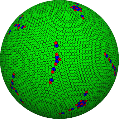
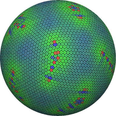
Figure 1: The configuration with the lowest observed energy for $s=1$ and $N=4352$ points generated by Wales, McKay and Altschuler Wales, McKay, and Altschuler (2009a). Each point is depicted as a dot on the surface of the sphere surrounded by its Voronoi cell, which we computed with QHull Barber, Dobkin, and Huhdanpaa (1996). In the image on the left the five sided cells are gray (red in the online version), the six sided cells are light gray (green in the online version) and the seven sided cells are dark gray (blue in the online version). The image on the right shows the same configuration in the same orientation, but with the Voronoi cells colored by point energy. (In the online version blue indicates the lowest point energies, green average point energies and red, the highest.) Note that the fluctuations in point energy extend out from the defects into the surrounding “hexagonal sea”.

A natural question to ask is: how much does the energy change as the structure and location of defects changes? Because stable configurations differ from the minimal configuration in location and structure of defects, a related question is: how much does the average energy of stable configurations differ from the true minimal energy? We answer this empirically by developing a large library of stable configurations and comparing the resulting average energy of the stable configurations with the lowest observed energy.

Minimal energy is often approximated in an asymptotic expansion, in $N$, and we compare the difference between the average and lowest observed energy with the terms in these asymptotic expansions. That is, we empirically identify the terms in the asymptotic expansion that approximate the lowest observed energy, but not the average energy. We believe that these terms likely reflect characteristics of defects.

This work has value in several ways. First, because the energy of any configuration of points on the sphere is an upper bound for the minimal energy, these results provide a lower bound for the difference between the average energy of stable configurations and the minimal energy. Second, there are methods that have a controllable error bound for quickly approximating the pairwise energy, most notably the Fast Multipole Method Greengard and Rokhlin (1987). For such approximations the results in this paper will help select the error bound necessary to distinguish stable configurations from minimal configurations. Finally, this work suggests which terms in the asymptotic expansion will require an understanding of defect structure.

The rest of the paper is organized as follows: Section II review some of the relevant work. Section III describes our method for generating stable configurations, and reports properties of these stable configurations. Section IV compares theory and conjecture with minimal observed energy and reports the observed asymptotic differences between the average energy of stable configurations and minimal observed energy. Additionally, we examine and extend some conjectures regarding the second order term for the Thomson problem. In Section V we summarize our results.

II Background

Some of the earliest computational work on the Thomson Problem was done by Erber and Hockney Erber and Hockney (1991, 1997) where they rely on optimization techniques to search for minimal energy configurations. Rakhmanov, Saff and Zhou Rakhmanov, Saff, and Zhou (1995) presented a comprehensive search for the minimal energies for $N$ up to $200$ for the logarithmic as well as Coulomb energies. Morris, Deavon and Ho Morris, Deaven, and Ho (1996) used a genetic algorithm in an effort to avoid becoming trapped in stable non-minimal configurations. An important effort to constructively generate candidate minimal energy configurations came from Altschuler, Williams, Ratner, Tipton, Stong, Dowla and Wooten Altschuler et al. (1997), where the authors of that paper identified configurations with twelve point defects and high symmetry. These configurations were later shown not to be minimal by Pérez-Garrido, Dodgson, Moore, Ortuno and Diaz-Sanchez Pérez-Garrido et al. (1997) and Pérez-Garrido, Dodgson, Moore PerezGarrido, Dodgson, and Moore (1997). These authors found that, as $N$ increased, the defects were not point defects, but had considerable structure such as those in Figure 1. Efforts to understand and characterize this structure, as well as find minimal energy configurations, include the work of Wales and Ulker Wales and Ulker (2006a) and Wales, McKay and Altschuler Wales, McKay, and Altschuler (2009a). The results of the experiments described in these two publications are collected in the Cambridge Cluster Database Wales and Ulker (2006b) Wales, McKay, and Altschuler (2009b), and provide, to our knowledge, the lowest observed energies for the Thomson Problem. Bowick, Cacciuto, Nelson and Travesset Bowick et al. (2006) use a continuum elasticity model to describe the interaction of defects. In these works the empirical evidence is that configurations with low energy consist of a “hexagonal sea” with complex defects at the vertices of an icosahedron inscribed in $\mathbb{S}^{2}$.

Theoretical examinations of the Thomson Problem provide valuable insights and language for the problem, and we review some of the relevant theory here. Let $\omega_{N}$ denote a set $\{{\bf x}_{1},\ldots,{\bf x}_{N}\}$ of $N$ distinct points in ${\mathbb{R}}^{p}$. We consider the following discrete energy of $\omega_{N}$

$$E_{s}(\omega_{N}):=\sum_{i=1}^{N}\sum_{j=1\,j\neq i}^{N}k_{s}(|{\bf x}_{i}-{\bf x}_{j}|),$$ (1)

where $k_{s}$ is the function given by

$$k_{s}(r)=\left\{\begin{array}[]{cc}r^{-s}&\text{for $s>0$}\\ -\log r&\text{for $s=0$},\end{array}\right.$$

and where $|\cdot|$ is the Euclidean norm inherited from ${\mathbb{R}}^{p}$. Note that many papers on this topic report an energy where the second sum is over $j=i+1,\ldots,N$ leading to a factor of two difference in our values for energy. The functions, $k_{s}$, are the Riesz potentials, which are a natural generalization of the Coulomb potential. The questions in which we are interested apply to Riesz potentials in general, and we present results for the Riesz potentials corresponding to $s=0$, $1$, $2$, and $3$. We denote the point ($s$-)energy of the $i^{\text{th}}$ point in $\omega_{N}$ by

$$U_{s}^{i,\omega_{N}}:=\sum_{j=1\,j\neq i}^{N}k_{s}(|{\bf x}_{i}-{\bf x}_{j}|)\quad\text{and then the total energy is given by}\quad E_{s}(\omega_{N})=\sum_{i=1}^{N}U_{s}^{i,\omega_{N}}.$$

For any compact set $A\subset{\mathbb{R}}^{p}$ of Hausdorff dimension $d>0$, the lower semi-continuity of $k_{s}$ ensures that there is at least one configuration contained in $A$, which we denote $\omega_{N}^{s,A}$, that satisfies

$$E_{s}(\omega_{N}^{s,A})={\mathcal{E}}_{s}(A,N):=\inf\{E_{s}(\omega_{N}):\omega_{N}\subset A\,\text{and}\,{\bf x}_{i}\neq{\bf x}_{j}\,\text{for all $i\neq j$}\}.$$

That is to say, there is at least one energy-minimizing configuration, $\omega_{N}^{s,A}$, and the minimal $N$-point $s$-energy is denoted ${\mathcal{E}}_{s}(A,N)$. In this setting one can search for an expansion of the minimal energy as a function of $N$ of the form

$${\mathcal{E}}_{s}(A,N)\approx C_{1}N^{\alpha_{1}}+C_{2}N^{\alpha_{2}}+\ldots.$$ (2)

In certain cases, e.g. $s=0$ and $s=d$, this expansion will also include logarithmic terms.

In the general case where $A$ is any $d$ dimensional compact set and $s<d$, Pólya and Szegö establish the first order term Pólya and Szegö (1931) by connecting the asymptotic behavior of the discrete minimal energy with a continuum problem. Specifically, let ${\mathcal{M}}(A)$ denote the positive Borel measures supported on $A$, and ${\mathcal{M}}_{1}(A)\subset{\mathcal{M}}(A)$ denote the Borel probability measures supported on $A$. One may interpret $\mu\in{\mathcal{M}}(A)$ as a continuous charge distribution and consider the energy functional defined for any $\mu\in{\mathcal{M}}(A)$, by

$$I_{s}(\mu):=\iint k_{s}(|{\bf x}-{\bf y}|)\,d\mu({\bf y})d\mu({\bf x}).$$

Analogous to the discrete point energy, $U_{s}^{i,\omega_{N}}$, the potential due to $\mu$ at a point ${\bf x}$, is

$$U_{s}^{\mu}({\bf x}):=\int k_{s}(|{\bf x}-{\bf y}|)\,d\mu({\bf y}),\quad\text{and then}\quad I_{s}(\mu):=\int U_{s}^{\mu}({\bf x})\,d\mu({\bf x}).$$

There is a unique energy-minimizing measure $\mu^{s,A}\in{\mathcal{M}}_{1}(A)$ so that

$$I_{s}(\mu^{s,A})<I_{s}(\mu)\quad\text{for all}\quad\mu\in{\mathcal{M}}_{1}(A)\backslash\{\mu^{s,A}\}.$$

(cf. (Landkof, 1973, pp. 131-133) also Götz Götz (2003) provides a proof of a key step without using standard Fourier techniques.) Further,

$$U_{s}^{\mu^{s,A}}({\bf x})=I_{s}(\mu^{s,A})$$ (3)

for all ${\bf x}\in\operatorname{supp}\mu^{s,A}$ with the possible exception of a set that supports no measures of finite energy (cf. (Fuglede, 1960, Theorem 2.4)). Roughly speaking Equation (3) asserts that the potential is constant in regions where there is charge. The essence of the proof is that, if this were not the case, energy could be decreased by moving charge from regions of high potential to regions of low potential.

The celebrated transfinite diameter result of Pólya and Szegö relates the continuous and discrete problems as follows (also cf. (Landkof, 1973, pp. 160-162)): for any continuous function $f:A\to\mathbb{R}$ and any sequence of energy-minimizing configurations $\{\omega_{N}^{s,A}\}_{N=2}^{\infty}$,

$$\lim_{N\to\infty}\frac{1}{N}\sum_{{\bf x}\in\omega_{N}^{s,A}}f({\bf x})=\int f\,d\mu^{s,A},$$

and

$$\lim_{N\to\infty}\frac{{\mathcal{E}}_{s}(A,N)}{N^{2}}=I_{s}(\mu^{s,A}).$$ (4)

For this range of $s$ the discrete minimal energy configurations are converging in the weak-star topology of measures to $\mu^{s,A}$. The minimal energy grows as $N^{2}$, where the coefficient is given by $I_{s}(\mu^{s,A})$. The proof of these results indicates that the first order approximation of the minimal energy is determined by the global distribution of points within energy minimizing configurations. Kuijlaars and Saff have shown Kuijlaars and Saff (1998) that the second order term on the sphere in the expansion (2) grows as $N^{3/2}$ and the, still to be proven, coefficient is conjectured to depend on the presumed local hexagonal structure.

If $s\geq d$, then $I_{s}(\mu)=\infty$ for all $\mu\in{\mathcal{M}}(A)\backslash\{0\}$, (cf. (Mattila, 1995, Ch. 8)) and other techniques are required to estimate growth in minimal energy. Hardin and Saff Hardin and Saff (2005) and Borodachov, Hardin and Saff Borodachov, Hardin, and Saff (2008) show that when $A$ has certain smoothness properties

$$\lim_{N\to\infty}\frac{1}{N}\sum_{{\bf x}\in\omega_{N}^{s,A}}f({\bf x})=\frac{1}{|{\mathcal{H}}^{d}_{A}|}\int f\,d{\mathcal{H}}^{d}_{A},$$

and

$$\lim_{N\to\infty}\frac{{\mathcal{E}}_{s}(A,N)}{N^{1+s/d}}=\frac{C_{s,d}}{{\mathcal{H}}^{d}(A)^{s/d}}\quad\text{for $s>d$, and}\quad\lim_{N\to\infty}\frac{{\mathcal{E}}_{d}(A,N)}{N^{2}\log N}=\frac{{\mathcal{H}}^{d}({\mathcal{B}}^{d})}{{\mathcal{H}}^{d}(A)},$$

where ${\mathcal{H}}^{d}_{A}$ is the $d$ dimensional Hausdorff measure restricted to $A$, $C_{s,d}$ is a constant that depends only on $d$ and $s$ and not the underlying set $A$, and ${\mathcal{B}}^{d}$ is the closed unit ball in ${\mathbb{R}}^{d}$. These results demonstrate that for $s\geq d$ the asymptotic distribution of points in energy-minimizing configurations is uniform. Furthermore, the minimal $N$-point energy grows at a rate exceeding $N^{2}$ and is determined largely by the local structure of the energy minimizing configurations. Indeed for the $d=2$ case, numerical evidence supports the conjecture that $C_{s,d}$ is given by a hexagonal zeta function evaluated at $s$, i.e. the sum of the reciprocal non-zero distances in the hexagonal lattice raised to the power $s$. Brauchart, Hardin and Saff present a summary of theory and conjecture regarding minimal energy configurations on the sphere Brauchart, Hardin, and Saff (2011).

III Numerical Methods

III.1 Generating Candidate Minimal Energy Configurations

To generate candidate configurations we begin with a random, well-separated, initial configuration of points on $\mathbb{S}^{2}$ and alternate between the Polak-Ribière variant of Conjugate Gradient (cf. Press et al. (1992)) with a line minimization of the energy, and an exact Newton’s Method to find a root of the gradient. To solve the linear system arising in Newton’s Method we use LAPACK Anderson and Dongarra (1993).

We use a direct evaluation of the energy sum, given in Equation (1) omitting obvious duplicate calculations, which involves $\mathcal{O}(N^{2})$ terms, the smallest of which is $k_{s}(2)$, while ${\mathcal{E}}_{s}(\mathbb{S}^{2},N)$ can grow into the hundreds of millions for some values of $s$ and $N$ considered. To control the numerical round-off error associated with adding two numbers whose ratio is far from unity (cf. Higham (1993) for relevant work on this problem) we logarithmically bin our summands. By only adding summands in the same bin, we bound the ratio of any two intermediate summands to be added. The final sum is computed by iterating over our bins in increasing magnitude and summing their contents.

For $N=20,\ldots,180$ we ran thousands of trials. For $N=181,\ldots,500,4352$ we ran tens to hundreds of trials. We report lowest observed energies on the sphere only for those $N$ where the Cambridge Cluster Database provides a configuration with which we can initialize our solver.

III.2 Generating Stable Configurations

The above optimization process leads to a candidate configuration $\omega_{N}$, which we assume is close enough to a true stable configuration $\bar{\omega}_{N}$ so that the linear approximation about $\omega_{N}$ for the gradient

$$0=\nabla E_{s}(\bar{\omega}_{N})\approx\nabla E_{s}(\omega_{N})+\nabla^{2}E_{s}(\omega_{N})(\bar{\omega}_{N}-\omega_{N})$$

is reasonable. Here $\nabla E_{s}$ is the gradient of the energy with respect to the free parameters that define $\omega_{N}$ and $\nabla^{2}E_{s}$ is the Hessian represented in the same coordinates. Were the Hessian invertible this would lead to the bound

$$\frac{\|\nabla E_{s}(\omega_{N})\|_{2}}{\lambda_{\text{min}}}=\|\nabla^{2}E_{s}(\omega_{N})^{-1}\|\,\|\nabla E_{s}(\omega_{N})\|_{2}\geq\|\bar{\omega}_{N}-\omega_{N}\|_{2}\geq\|\bar{\omega}_{N}-\omega_{N}\|_{\infty},$$

where $\lambda_{\text{min}}$ is the smallest eigenvalue of the Hessian, $\|\cdot\|_{2}$ is the unnormalized two-norm of the parameters defining the argument, and $\|\cdot\|$ is the associated operator two-norm. Our choice of coordinates leads to three degrees of freedom corresponding to rigid motions of the sphere and so the smallest three eigenvalues of the Hessian are zero. We assume a rotation and reflection of $\bar{\omega}_{N}$ so that the difference between $\bar{\omega}_{N}$ and $\omega_{N}$ and does not reflect these rigid motions. We let $\lambda^{*}_{\text{min}}$ denote the fourth lowest eigenvalue, then we have the bound

$$\frac{\|\nabla E_{s}(\omega_{N})\|_{2}}{\lambda^{*}_{\text{min}}}\geq\|\bar{\omega}_{N}-\omega_{N}\|_{\infty}.$$

We desire that

$$\|\bar{\omega}_{N}-\omega_{N}\|_{\infty}\leq\frac{\min_{i\neq j\in 1,\ldots,N}|{\bf x}_{i}-{\bf x}_{j}|}{10,000}$$

Our reasoning is that the free parameters are the polar and azimuthal angles, and, on the unit sphere, changes in position are always bounded from above by changes in angle. The above bound will ensure that no point in $\omega_{N}$ is further from its corresponding point in the true stable state by more than the arbitrary bound of one ten-thousandth of the minimum separation in $\omega_{N}$. This is ensured if

$$\frac{\|\nabla E_{s}(\omega_{N})\|_{2}}{\lambda^{*}_{\text{min}}}\leq\frac{\min_{i\neq j\in 1,\ldots,N}|{\bf x}_{i}-{\bf x}_{j}|}{10,000},$$ (5)

where, again, we used LAPACK to compute $\lambda^{*}_{\text{min}}$. We reiterate that these estimates hinge on the assumption that the gradient at the true stable state is well approximated by a linear expansion of the gradient about the observed state. We keep candidate configurations if Equation (5) holds or if the configuration possesses the lowest observed energy.

Note that Equation (5) is quite stringent. As $N$ increases, the minimum pairwise separation between points goes as $N^{-1/2}$. In addition we have bounded from above the infinity-norm with the unnormalized two-norm. Such a bound is tight only when all the components but one are zero. This condition was relaxed for $N=4352$, where we simply required that all but lowest three eigenvalues be positive.

III.3 Properties of Stable Configurations

In Figure 2 one can see the average fraction of points that have six-sided Voronoi cells. For each $N$ and $s$, these data are obtained by computing this fraction per configuration, and then averaging over all the observed configurations and weighting by the number of times the configuration occurred. This is the same averaging method we use when computing the average energy of stable configurations. As one can see this average fraction is better than $91$ percent for $N\geq 200$, supporting the claim that stable configurations are largely hexagonal.

As a point of comparison, we’ve also computed this fraction for the configurations that have the lowest observed energy. This is shown in Figure 3. One important feature of this plot is that the configurations with the lowest observed energy have far more non-six-sided Voronoi cells than the minimum allowed if no Voronoi cell has fewer than five sides. If one further assumes that no Voronoi cell has more than seven sides, then the number of Voronoi cells with other than six sides must be even. This corroborates previous observation that as $N$ increases, the defects cease to be single points and develop structure.

Figure 2: This plot shows the fraction of points that have six-sided Voronoi cells for $N$ and for the values of $s$ in which we are interested. The inset plot provides more detail for $N=200,\ldots,500$. In addition we’ve plotted the upper bound for this fraction assuming that no Voronoi cell has fewer than five sides. Each data point is averaged over all the configurations, weighted by number of occurrences, for the specified $N$ and $s$.

Figure 3: As in Figure 2 we’ve plotted the fraction of points that have six-sided Voronoi cells. Here each data point corresponds to the configuration with the lowest observed energy. In the outer plot the solid line is the upper bound on this fraction, while the dashed line indicates what this fraction would be if there were $12$ defects each consisting of a three points with five, seven and five sided Voronoi cells respectively. In the inset one sees lines corresponding to $12,14,16,\ldots,36$ non six-sided Voronoi cells.

IV Asymptotics of Minimal Energy and Average Energy of Stable Configurations

In this section we compare theory and conjecture for the minimal $N$-point energy with the lowest observed $N$-point energy. In the case $s=1$ we extend a conjecture for the second order term on $\mathbb{S}^{2}$ to certain smooth manifolds. We report the asymptotics of the difference between the average and minimal observed energies and compare this difference with terms in the asymptotic expansion.

Like all computational works of this type, we have no assurances that the lowest available energies are indeed minimal. Systematic errors of this type would cause us to underestimate the difference between the average and the minimal energies. Consequently our results that indicate that a term in the asymptotic expansion does not describe both the average and minimal energy should be trusted more than results indicate that a term does describe both the average and minimal energies.

We shall use the following notation: $\tilde{\mathcal{E}}_{s}(A,N)$ is the lowest observed minimal $N$-point $s$-energy on a set $A$. $R_{s}^{n}(A,N)$ is the difference between the minimal $N$-point $s$-energy on $A$ and an $n$-term asymptotic expansion of the minimal $s$-energy, while $\tilde{R}_{s}^{n}(A,N)$ is the difference between the lowest observed energy and the $n$-term expansion.

IV.1 The $s=1$ Case

This is the Thomson Problem, and the leading order term in the asymptotic expansion of the minimal energy follows from the transfinite diameter result in Equation (4), i.e. for a set $A$ of dimension $d>1$ it is $I_{1}(\mu^{1,A})N^{2}$. For the sphere a simple calculation shows that $I_{1}(\mu^{1,\mathbb{S}^{2}})=1$. We now review an existing conjecture for the second order term on $\mathbb{S}^{2}$, and show how it may be generalized for compact $2$-manifold $A$. A trivial representation of the first order term and the correction for a set $A$ is

$${\mathcal{E}}_{1}(A,N)=I_{1}(\mu^{1,A})N^{2}+\sum_{i=1}^{N}\left(\sum_{j\neq i}\frac{1}{|{\bf x}_{i}-{\bf x}_{j}|^{s}}-I_{1}(\mu^{1,A})N\right).$$ (6)

We shall consider the case that $\mu^{1,A}$ is absolutely continuous with respect to ${\mathcal{H}}^{d}_{A}$, the support of $\mu^{1,A}$ is all of $A$, and Equation (3) holds for the entire support of $\mu^{1,A}$, that is $U_{s}^{\mu^{1,A}}({\bf x})=I_{s}(\mu^{s,A})$ for all ${\bf x}\in A$. These assumptions are satisfied for $A=\mathbb{S}^{2}$.

The potential $U_{s}^{\mu}$ is linear in $\mu$ and so, with our assumptions, we may write Equation (6) as

$${\mathcal{E}}_{1}({A},N)=I(\mu^{1,A})N^{2}+\sum_{i=1}^{N}\left(\sum_{j\neq i}\frac{1}{|{\bf x}_{i}-{\bf x}_{j}|}-U_{1}^{N\mu^{1,A}}({\bf x}_{i})\right).$$ (7)

The above equation is exact regardless of where on $A$ we choose to evaluate the potential $U_{1}^{N\mu^{1,A}}$. However, choosing to evaluate the potential at the points that form a minimal $N$-point configuration suggests one way to express the correction: the point energy for ${\bf x}_{i}$ should be corrected by subtracting the potential at ${\bf x}_{i}$ due to $N$ times the equilibrium measure and adding the energy due to the presence of the $N-1$ other discrete points. In broader terms the point at ${\bf x}_{i}$ sees other discrete points, not a smoothed out average density.

For the $i^{\text{th}}$ point, the correction given by Equation (7) may be written as two terms, which we refer to as “near” and “far” contributions.

$$\sum_{j\neq i}\frac{1}{|{\bf x}_{i}-{\bf x}_{j}|}-U_{1}^{N\mu^{1,A}}({\bf x}_{i}) =\displaystyle{\left(\sum_{j\neq i}\frac{\exp(-|{\bf x}_{i}-{\bf x}_{j}|/R)}{|{\bf x}_{i}-{\bf x}_{j}|}-\int\frac{\exp(-|{\bf x}_{i}-{\bf y}|/R)}{|{\bf x}_{i}-{\bf y}|}d\mu^{1,A}({\bf y})\right)}$$

$$+\displaystyle{\left(\sum_{j\neq i}\frac{1-\exp(-|{\bf x}_{i}-{\bf x}_{j}|/R)}{|{\bf x}_{i}-{\bf x}_{j}|}-\int\frac{1-\exp(-|{\bf x}_{i}-{\bf y}|/R)}{|{\bf x}_{i}-{\bf y}|}d\mu^{1,A}({\bf y})\right)}$$

This decomposition is motivated by the reasoning presented by Kuijlaars and Saff (Kuijlaars and Saff, 1998, Section 2), namely that the second order correction for $0<s<2$ is determined by the local structure. Where Kuijlaars and Saff use a cutoff at radius $R$, we use an exponential damping that allows use of the Poisson Summation Formula and Ewald type arguments for the $s=1$ case.

We fix $R>0$ small enough so that $d\mu^{s,A}/d{\mathcal{H}}^{d}_{A}$ changes on a scale much larger than $R$, and we consider $N$ large enough so that the nearest neighbor distance is much smaller than $R$. Then for most $i$ we can expect a local hexagonal structure around ${\bf x}_{i}$ and so we consider the following estimate for the near term in Equation (IV.1):

$$N^{-1/2}\left(\sum_{j\neq i}\frac{\exp(-|{\bf x}_{i}-{\bf x}_{j}|/R)}{|{\bf x}_{i}-{\bf x}_{j}|}-\int\frac{\exp(-|{\bf x}_{i}-{\bf y}|/R)}{|{\bf x}_{i}-{\bf y}|}d\mu^{1,A}({\bf y})\right)$$

$$\approx N^{-1/2}\left(\sum_{{\bf x}\in D_{i}N^{-1/2}\Lambda\backslash\{0\}}\frac{\exp(-|{\bf x}|/R)}{|{\bf x}|}-\frac{1}{|D_{i}N^{-1/2}\Lambda|}\int_{{\mathbb{R}}^{2}}\frac{\exp(-|{\bf x}|/R)}{|{\bf x}|}d^{2}{\bf x}\right)$$ (9)

Here $\Lambda:=\{m{\bf r}_{1}+n{\bf r}_{2}:{\bf r}_{1}=(1,0),\,{\bf r}_{1}=(1/2,\sqrt{3}/2)\,\text{and}\,m,n\in\mathbb{Z}\}$ is the hexagonal lattice of unit spacing, $D_{i}\Lambda$ is the hexagonal lattice where the generating vectors have been scaled by $D_{i}$, and $|D_{i}\Lambda|=\sqrt{3}D_{i}^{2}/2$ is the area of the fundamental cell of the scaled lattice. Finally, $d^{2}{\bf x}$ denotes integration with respect to area. The essential statement of the approximation in Equation (9) is that, for most points in a configuration with low energy, the energy due to neighboring points is well approximated by the energy due to the neighboring points in an appropriately scaled hexagonal lattice, and that the density represented by equilibrium measure changes little on the scale of nearest neighbor separation. This assumption is qualitatively supported by Figure 1 where most points are surrounded by a local hexagonal structure.

We compute the sum over a lattice that is scaled by $D_{i}N^{-1/2}$, which is intended to reflect the local point density of the energy minimizing configuration near the point ${\bf x}_{i}$. For the case $A=\mathbb{S}^{2}$, $D_{i}$ is independent of $i$. To generalize to an arbitrary 2-manifold one may estimate $D_{i}$ as follows: Let $r$ be the nearest-neighbor spacing. Assume that for large $N$, hence small $r$, the Voronoi cells within $B({\bf x}_{i},r_{0})$ are all hexagonal and of the same size. This gives

$$\#\left(\omega_{N}^{s,A}\cap B({\bf x}_{i},r_{0})\right)H_{r/2}\approx{\mathcal{H}}^{2}_{A}(B({\bf x}_{i},r_{0})).$$ (10)

Here $\#$ indicates the number of points in the following set. $H_{r/2}$ is the area of a hexagon of inner radius $r/2$, which is $\sqrt{3}r^{2}/2$.

The second estimate follows from the weak-star convergence of the discrete minimal energy points to the equilibrium measure and the assumption that $A\cap B({\bf x}_{i},r_{0})$ is $\mu^{1,A}$-almost clopen. Then, for $N$ sufficiently high,

$$\frac{\#\left(\omega_{N}^{s,A}\cap B({\bf x}_{i},r_{0})\right)}{N}\approx\mu^{1,A}(B({\bf x}_{i},r_{0})).$$ (11)

Dividing (11) by (10) gives, for $N$ sufficiently large

$$\frac{2}{\sqrt{3}r^{2}N}=\frac{\mu^{1,A}(B({\bf x}_{i},r_{0}))}{{\mathcal{H}}^{2}_{A}(B({\bf x}_{i},r_{0}))}.$$

As $r_{0}$ decreases to zero, the right hand side tends toward the Radon-Nikodým derivative of $\mu^{1,A}$ with respect to ${\mathcal{H}}^{2}_{A}$ and we have that the nearest neighbor spacing $r$, and the appropriate scaling for the lattice at ${\bf x}_{i}$, is given by

$$r=\sqrt{\frac{2}{\sqrt{3}N}\left(\frac{d\mu^{1,A}}{d{\mathcal{H}}^{2}_{A}}({\bf x}_{i})\right)^{-1}}\qquad\text{hence}\qquad D_{i}=\sqrt{\frac{2}{\sqrt{3}}\left(\frac{d\mu^{1,A}}{d{\mathcal{H}}^{2}_{A}}({\bf x}_{i})\right)^{-1}}$$

With some substitutions, the limit as $N$ grows to infinity of (9) may be expressed as

$$\frac{1}{D_{i}}\lim_{R\to\infty}\left(\sum_{{\bf x}\in\Lambda\backslash\{0\}}\frac{\exp(-|{\bf x}|/R)}{|{\bf x}|}-\frac{1}{|\Lambda|}\int_{{\mathbb{R}}^{2}}\frac{\exp(-|{\bf x}|/R)}{|{\bf x}|}d^{2}({\bf x})\right)$$ (12)

We evaluate this limit (omitting the factor $1/D_{i}$) in the appendix as $-2.10671$ and denote its value as $C$.

Discarding the far piece in Equation (IV.1), assuming a local hexagonal structure, and replacing the outer sum with an integral on the right hand side of Equation (7) gives the following conjecture.

Conjecture IV.1.

Let $A$ be a compact $2$-manifold where $\mu^{1,A}$ is absolutely continuous with respect to ${\mathcal{H}}^{d}_{A}$, where the support of $\mu^{1,A}$ is all of $A$, and where $U_{1}^{\mu^{1,A}}({\bf x})=I_{s}(\mu^{s,A})$ for all ${\bf x}\in A$. Then

$$\lim_{N\to\infty}\frac{{\mathcal{E}}_{1}({A},N)-I_{1}(\mu^{1,A})N^{2}}{N^{3/2}}=C\sqrt{\frac{\sqrt{3}}{2}}\int\sqrt{\frac{d\mu^{1,A}}{d{\mathcal{H}}^{2}_{A}}({\bf x})}\,d\mu^{1,A}({\bf x}),$$ (13)

where

$$C=\lim_{R\to\infty}\left(\sum_{{\bf x}\in\Lambda\backslash\{0\}}\frac{\exp(-|{\bf x}|/R)}{|{\bf x}|}-\frac{1}{|\Lambda|}\int_{{\mathbb{R}}^{2}}\frac{\exp(-|{\bf x}|/R)}{|{\bf x}|}d^{2}({\bf x})\right),$$

and where $\Lambda$ is the unit hexagonal lattice.

Conjecture IV.1 follows from a number of simplifying and possibly unnecessary assumptions. A broader conjecture that is closer in form to Conjecture 2 given by Kuijlaars and Saff Kuijlaars and Saff (1998) is

Conjecture IV.2.

Let $A$ be a compact $2$-manifold, $0<s<2$, and $\mu^{s,A}$ absolutely continuous with respect to ${\mathcal{H}}^{d}_{A}$, then

$$\lim_{N\to\infty}\frac{{\mathcal{E}}_{s}({A},N)-I_{s}(\mu^{s,A})N^{2}}{N^{1+s/2}}=C_{s}\int\sqrt{\frac{d\mu^{s,A}}{d{\mathcal{H}}^{2}_{A}}({\bf x})}\,d\mu^{s,A}({\bf x}),$$

where

$$C_{s}=6\left(\frac{\sqrt{3}}{8\pi}\right)^{s/2}\zeta(s/2)L_{-3}(s/2).$$

Here $\zeta$ is the analytic extension of the Riemann Zeta function and $L_{-3}$ is the Dirichlet L-function given by

$$L_{-3}(\alpha)=1-\frac{1}{2^{\alpha}}+\frac{1}{4^{\alpha}}-\frac{1}{5^{\alpha}}+\frac{1}{7^{\alpha}}\cdots$$

Conjectures IV.1 and IV.2 both predict $2.0\times-0.553051$ for the coefficient of the $N^{3/2}$ term on $\mathbb{S}^{2}$, and are in good agreement with energies on the sphere.

We now consider two additional numerical tests of these conjectures. In the first test we shall look at the torus $\mathbb{T}^{2}$ using a modest data set of low energy configurations. However, we also need an approximation of $\mu^{1,\mathbb{T}^{2}}$, and we turn to the work of Brauchart, Hardin and Saff on sets of revolution Brauchart, Hardin, and Saff (2009). In that work the authors begin with the fact that for sets of revolution, the equilibrium measure must be invariant under revolution. They develop a lower dimensional minimization problem on the set, which when rotated, gives $A$. While the theory does not address the case $s=1$, we use their theory as a recipe to approximate $\mu^{1,\mathbb{T}^{2}}$ numerically and present the results in Table 1.

We denote the torus of major radius $l$ and minor radius $a$ by $\mathbb{T}^{2}(l,a)$. Landkof (Landkof, 1973, p. 166) provides the following formula for the energy of the equilibrium measure on the torus:

$$I_{1}\left(\mu^{1,\mathbb{T}^{2}(l,a)}\right)=\frac{2c}{\pi^{2}}\left[\frac{Q_{-1/2}\left(\frac{l}{a}\right)}{P_{-1/2}\left(\frac{l}{a}\right)}+2\sum_{n=1}^{\infty}\frac{Q_{n-1/2}\left(\frac{l}{a}\right)}{P_{n-1/2}\left(\frac{l}{a}\right)}\right],$$ (14)

where $c=\sqrt{l^{2}-a^{2}}$ and where $P_{\nu}$ and $Q_{\nu}$ are Legendre functions of the first and second kind. We use the GNU Scientific Library Galassi et al. (2009) to evaluate the Legendre functions in the above sum. In Table 1 we see good agreement between the energies that result from extending the work in Brauchart, Hardin, and Saff (2009) to $s=1$ and the energies given by (14). Because the equilibrium measure is the unique measure that minimizes the energy, we conclude that the measure generated by applying the theory in Brauchart, Hardin, and Saff (2009) to the torus for $s=1$ generates a reasonable approximation of the equilibrium measure on the torus. Further, our numerical experiments show that the support of the equilibrium measure is $\mathbb{T}^{2}(l,a)$. In Figure 4 we plot the difference between the observed minimal energy and the first order term, i.e. $\tilde{R}_{1}^{1}(A,N)$. We also plot the conjectured value for the $N^{3/2}$ term using our numerical approximation of $\mu^{1,\mathbb{T}^{2}}$. The agreement suggests that Conjectures IV.1 and IV.2 appears to hold for the torus.

$A$	$M$	Energy computed using Brauchart, Hardin, and Saff (2009)	Energy computed with Equation (14)	Relative error
$\mathbb{T}^{2}(1.5,1)$	$1000$	$0.4782545$	$0.47825526366953$	$1.597\times 10^{-6}$
$\mathbb{T}^{2}(2,1)$	$1000$	$0.411239$	$0.41123994225477$	$2.291\times 10^{-6}$
$\mathbb{T}^{2}(3,1)$	$950$	$0.3234383$	$0.323438867490233$	$1.754\times 10^{-6}$

Table 1: A comparison of the $s=1$ energy of the equilibrium energy computed in two ways on three different tori. The first method uses the work of Brauchart, Hardin and Saff Brauchart, Hardin, and Saff (2009) as a recipe for approximating the $s=1$ equilibrium measure. The second method uses Equation (14). $M$ is the dimension of the discretized problem arising from Brauchart, Hardin, and Saff (2009).

Figure 4: A plot of $\tilde{R}^{1}_{1}(A,N)$ for $A=\mathbb{T}^{2}(1.5,1)$, $A=\mathbb{T}^{2}(2,1)$ and $A=\mathbb{T}^{2}(3,1)$. For each manifold, we’ve overlaid the prediction for the $N^{3/2}$ term given by Conjectures IV.1 and IV.2.

We do not have a model beyond the second term. However, our data suggest the form of higher order terms. In Figure 5 we’ve plotted the difference between the observed lowest energy and the first two terms obtained from the transfinite diameter argument and Conjecture IV.1, i.e. $\tilde{R}^{2}_{1}(A,N)$. We see strong evidence that the third term is linear. We fit $\tilde{R}^{2}_{1}(A,N)$ to $\alpha N+\beta\sqrt{N}$ and report the values of $\alpha$ and $\beta$ in Table 2. To assign a goodness of fit we would need to be able to estimate the error in our estimates for the minimal energy. However, useful estimates of such errors from above are at least as hard as the formidable task of bounding from below the minimal energy.

$A$	$\alpha$	$\beta$
$\mathbb{S}^{2}$	0.05123	-0.3207
$\mathbb{T}^{2}(1.5,1)$	-0.0616	-0.3633
$\mathbb{T}^{2}(2,1)$	-0.0462	-0.7379
$\mathbb{T}^{2}(3,1)$	-0.02780	-0.6208

Table 2: Parameters from a best fit of $\alpha N+\beta\sqrt{N}$ to $\tilde{R}^{2}_{1}(A,N)$.

Figure 5: A plot of $\tilde{R}^{2}_{1}(A,N)$ for $A=\mathbb{S}^{2}$, $A=\mathbb{T}^{2}(1.5,1)$, $A=\mathbb{T}^{2}(2,1)$ and $A=\mathbb{T}^{2}(3,1)$. For each manifold we’ve overlaid the best fit of the form $\alpha N+\beta\sqrt{N}$.

Conjectures IV.1 and IV.2 are expressed in terms of an integral over the equilibrium measure and a coefficient derived from a sum over a hexagonal lattice. The formulation of these conjectures does not make any assumption about the location or structure of the defects. This would imply that, if stable configurations differ from the minimal configuration only in the structure and location of defects, then Conjectures IV.1 and IV.2 should approximate the average stable energy as well. This is our second test of the conjectures. In the top of Figure 6 we see that the difference between the average energy of stable configurations and the lowest observed energy is bounded by three ten-thousandths of the conjectured $N^{3/2}$ term. In the bottom of Figure 6 we see that this difference between the average and minimal energies is substantially larger when compared to the empirically obtained linear term ($.05123N$) for the minimal energy. Indeed for our data at $N=4352$ the average and minimal energy differ by 30% of the linear term.

The conclusion is that the first and second terms given by the transfinite diameter and the conjectured $N^{3/2}$ term will predict energies of stable and minimal configurations well, but the empirically obtained linear third term reflects properties of the minimal configuration that are absent in the stable configurations. We assume that these properties are the location and structure of the defects.

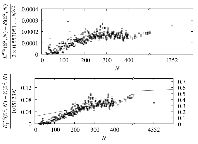
Figure 6: The top plot shows the difference between the average energy of stable configurations and the minimal observed energy divided by the conjectured $N^{3/2}$ term. In both plots the $x$ axis is broken to effectively display the data point at $N=4352$. The bottom plot shows the same energy difference divided by the empirically obtained linear third term. We have rescaled the right section of the lower plot and included a single line, plotted in both scales as reference. The error bars in this plot, and following plots of this type, are the standard error of the mean of the energy of the stable configurations.

IV.2 The $s=0$ Case

The problem of minimizing the $s=0$ energy is equivalent to the problem of maximizing the product of pairwise distances of points, and has received considerable attention from the mathematics community. The seventh of Smale’s eighteen problems for the twenty first century Smale (2000) is to develop an algorithm that will generate rapidly a configuration, $\omega_{N}^{*}$, that satisfies $E_{0}(\omega_{N}^{*})-{\mathcal{E}}_{0}(\mathbb{S}^{2},N)<C\log N$ for some constant $C$ that does not depend on $N$.

One challenge in solving this problem is estimating ${\mathcal{E}}_{0}(\mathbb{S}^{2},N)$ to at least ${\mathcal{O}}(\log N)$. Rakhmanov, Saff and Zhou made progress in this direction by bounding the linear term (Rakhmanov, Saff, and Zhou, 1994, Theorems 3.1 and 3.2) by defining $C_{N}$ as

$${\mathcal{E}}_{0}(\mathbb{S}^{2},N)=-\frac{1}{2}\log\left(\frac{4}{e}\right)N^{2}-\frac{1}{2}N\log N+C_{N}N,$$ (15)

and showing

$$-.225537540\ldots\leq\liminf_{N\to\infty}C_{N}\quad\text{and}\quad\limsup_{N\to\infty}C_{N}\leq-.04699460\ldots$$

In the same paper, those authors conjecture that

$${\mathcal{E}}_{0}(\mathbb{S}^{2},N)=-\frac{1}{2}\log\left(\frac{4}{e}\right)N^{2}-\frac{1}{2}N\log N+\alpha N+\beta\log N+{\mathcal{O}}(1).$$ (16)

We fit

$$-\frac{1}{2}\log\left(\frac{4}{e}\right)N^{2}-\frac{1}{2}N\log N+\alpha N+\beta\log N+\gamma$$

to our minimal energies and find a best fit for $\alpha=-0.0547$, $\beta=.6000$ and $\gamma=-2.680$. The value of $\alpha$ we obtain is in reasonable agreement with the value of $-0.052844$ obtained empirically by Brauchart, Hardin and Saff Brauchart, Hardin, and Saff (2011), and in stronger agreement with the value of $-0.055605\ldots$ given in Conjecture 4 Brauchart, Hardin, and Saff (2011).

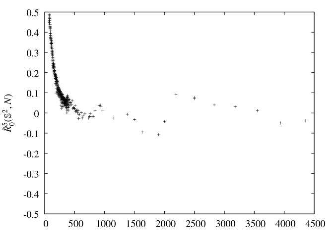
Figure 7: This is the observed minimal logarithmic energy minus a five term asymptotic expansion for the minimal energy. We see evidence of a term that decreases with $N$.

We fit over a range of $N=501,\ldots,4352$ because the data with which we have to work has behavior for $N\leq 500$ that is not captured in Equation (16). We plot the difference of the observed lowest energy and the five term asymptotic expansion in Figure 7. It is worth noting that, for $N>500$, the magnitude of this five term residual is less than $.2$ while the value of ${\mathcal{E}}_{0}(\mathbb{S}^{2},4352)$ is about $-3.6$ million.

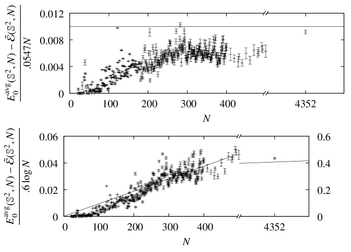
Figure 8: The top plot shows the difference of the average and lowest observed $s=0$ energies divided by the linear term in an asymptotic expansion. The bottom plots shows the same difference divided by the logarithmic term.

In Figure 8 we compare the difference between the average and minimal observed energies with the terms in the asymptotic expansion. For the data available, this energy difference is bounded by about one percent of the empirically obtained linear term, as is shown in the top plot. That is, the difference between the average energy of the stable configurations and the minimal observed energy is growing roughly as $N/2000$. It is worth comparing this with Figure 2 of Rakhmanov, Saff, and Zhou (1994) where the energy of constructively generated spiral point configurations differs from an estimate of the minimal energy by roughly $N/500$.

The qualitative interpretation that the data in the upper plot in Figure 8 are bounded while the data in the lower plot are growing implies that the first three terms in the asymptotic expansion describe the energy of stable configurations as well as the energy of minimal configurations, while the logarithmic term in the asymptotic expansion will reflect properties of the minimal configurations that are absent in most stable configurations. This implies that solving Smale’s seventh problem will require some understanding of the defects.

IV.3 The $s=2$ Case

Figure 9: The top plot shows the residual after the three term expansion given by Conjecture 5 from Brauchart, Hardin, and Saff (2011). The bottom plot shows the residual with three additional terms.

The Riesz kernel $k_{2}$ is not locally integrable on a $2$-manifold and the potential theoretic arguments cannot provide a first order term. Initial results for the leading order term on the sphere are given by Kuijlaars and Saff (Kuijlaars and Saff, 1998, Theorem 3). These results were generalized to a class of sets that include $C^{1}$ manifolds by Hardin and Saff (Hardin and Saff, 2005, Theorem 2.4). Combining these results with Conjecture 5 from Brauchart, Hardin, and Saff (2011), one has an asymptotic expansion of the form

$${\mathcal{E}}_{2}(\mathbb{S}^{2},N)=\frac{1}{4}N^{2}\log N+\alpha N^{2}+{\mathcal{O}}(1)$$

The conjectured value for $\alpha$ is $-0.08576841030090248365\ldots$

We fit the available data to

$$\frac{1}{4}N^{2}\log N+\alpha N^{2}+\varepsilon$$

and find that $\alpha=-0.085079$. However, the difference between the observed minimal energies and the best fit, shown in the top of Figure 9, has considerable structure. One hypothesis is that the form of the expression used for the fit is not correct. Making the arbitrary decision to include the same sequence of terms found in the expansion for the logarithmic energy, we fit

$$\frac{1}{4}N^{2}\log N+\alpha N^{2}+\beta N\log N+\gamma N+\delta\log N+\varepsilon$$

to our data, and when we fit the above, we found $\alpha=-0.085417$ and $\beta=.4415$. The residuals associated with the best fit of this augmented asymptotic expansion is shown in the lower plot of Figure 9.

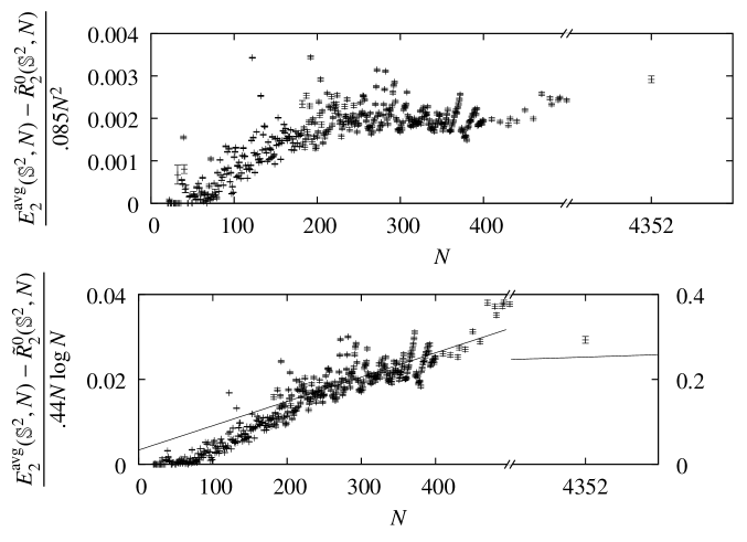
Figure 10: These two plots are the ratios of the difference between the average energy of stable configurations and the minimal observed energy to two terms in the asymptotic expansion for the energy. The top plot shows this difference compared to the empirically obtained $N^{2}$ and the bottom plot compares this difference with the empirically obtained $N\log N$ term.

Figure 10 shows the growth of the difference between the average energy of stable configurations with the minimal observed energy divided by the $N^{2}$ term in the top plot and an empirically obtained $N\log N$ term in the bottom plot. If one accepts that the data in the top plot is bounded, and the data in the bottom plot is growing, then one would conclude that the first two terms in the asymptotic expansion for the $s=2$ energy describe the energy of stable configurations as well as the minimal energy to about three parts in one thousand, while the next term, possibly an $N\log N$ term, would reflect properties of the minimal configurations absent in most stable configurations.

IV.4 The $s=3$ Case

Figure 11: The difference between the observed minimal $s=3$ energy and the two term expansion for the $s=3$ energy.

The Riesz kernel $k_{3}$, like $k_{2}$, is not locally integrable on $2$-manifolds. Early progress toward the leading order term for the asymptotic expansion of minimal $N$-point energy on the sphere (Kuijlaars and Saff, 1998, Theorem 2) shows that, if the leading order term exists for any $s>d$, the leading order term has the form $N^{1+s/2}$. Kuijlaars and Saff further conjecture that

$$\lim_{N\to\infty}\frac{{\mathcal{E}}_{s}(\mathbb{S}^{2},N)}{N^{1+s/2}}=\left(\frac{\sqrt{3}}{8\pi}\right)^{s/2}\zeta_{\Lambda}(s)=:\alpha$$ (17)

where $\Lambda$ is again the hexagonal lattice and $\zeta_{\Lambda}$ is the associated zeta function – the sum of the reciprocals of the non-zero distances in $\Lambda$ raised to the argument. The existence of the limit in (17), and hence the first order term, was established for a broad class of sets by Hardin and Saff Hardin and Saff (2005) and strengthened by Borodachov, Hardin and Saff Borodachov, Hardin, and Saff (2008), although the value of the limit has still not been proven. The natural assumption of a local hexagonal structure is implicit in the conjecture as $\Lambda$ is the hexagonal lattice. We compute this leading term, via the factorization presented Kuijlaars and Saff (1998) to get a value of $\alpha=2.0\times 0.0998139\ldots$. The second order term is conjectured (Brauchart, Hardin, and Saff, 2011, Conjecture 3) to be $\beta N^{2}$ where $\beta$ is given as the analytic extension, in $s\in\mathbb{C}$, of $I_{s}(\mu^{s,\mathbb{S}^{2}})$ to the case $s=3$. Following (Brauchart, Hardin, and Saff, 2011, Equation 10) we compute the coefficient as $\beta=-.25$.

Fitting the expression

$$\alpha N^{1+3/2}+\beta N^{2},$$ (18)

with $\alpha$ fixed at the value given in (17), to our data for $N=20,\ldots,4352$ gives a value of $\beta=-0.22\ldots$. The addition of terms of the form $\gamma N^{1.5}+\delta N+\varepsilon N^{.5}$ does not substantially change the value for $\beta$ obtained through such a fitting procedure. If we fit Expression (18) to the data and let $\alpha$ vary we obtain $\alpha=2.0\times 0.099878$ and $\beta=-0.2349\ldots$.

The difference between the observed lowest energy and the fit, shown in Figure 11 shows considerable structure, suggesting that either the form to which we fit is not correct, or that the energies with which are working are not minimal.

We plot the difference between the average and minimal energies in Figure 12. The upper plot suggests that this difference is small compared to the leading order term. The lower plot compares this difference to the conjectured second order term. This difference is about $4$ percent of the conjectured second order term at $N=4352$. However, the difference between the empirically obtained coefficient for the second order term and the conjectured coefficient is $12$ percent of the conjectured second order term. If our measurement of the second order coefficient differs from the conjectured value because our lowest observed energies are not the minimal energies, then the minimal energies differ from the lowest observed energies by several times the difference between the average and minimal energies.

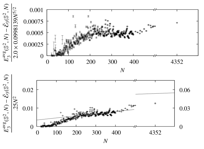
Figure 12: Here we present, in the top plot, the difference between the average of the $s=3$ energies of stable configurations and the minimal observed $s=3$ energy divided by the leading order ($N^{5/2}$) term estimate. The bottom plot shows the difference between the highest and lowest observed energies divided by the difference between the observed and conjectured second order term.

V Conclusions

We’ve used numerically generated candidates for $s$-energy minimizing configurations to assess conjectures for higher order terms in asymptotic expansions for the minimal $s$-energy. In addition we’ve developed a large library of stable configurations and compared the average of the energies of the stable configurations with the energies of the candidate minimal configurations to approximate a lower bound on the difference between the average and minimal energy.

V.1 Comparison of conjecture and numerical experiment

For $s=1$ we find that existing conjectures for the second order term on the sphere appear appear to hold when extended to the torus, and that the third term appears to be linear. For the sphere a straightforward fit suggests a value of $0.0513$ as the coefficient of this linear term. For $s=0$ the conjectured forms for the asymptotic expansion gave rise to an expression that agreed, for $N>500$, with our observed minimal energies to one part in thirty million. Using a fit for the linear term gives a value of $-0.0547$, while the conjectured value is $-0.055605\ldots$. For $s=2$ the conjectured form of the asymptotic expansion left considerable structure, suggesting that either the form of the fit was wrong or that the energies with which we had to work were not minimal. Two fits, assuming different forms of the asymptotic expansion, gave values for the coefficient of the conjectured second order $N^{2}$ term of $-0.085079$ and $-0.085417$. The conjectured value is $-0.085768\ldots$ For $s=3$, the conjectured coefficient of the first order term is $2.0\times 0.0998139\ldots$, while fitting our data gives $2.0\times 0.099856\ldots$. The second order term is conjectured to be $-.25N^{2}$. Fitting our data suggests a coefficient of $-.22$.

V.2 Identification of terms that likely reflect defect structure

For $s=1$ the difference between the average and lowest observed energy was small compared to the $N^{3/2}$ term, and appeared to be growing compared to an empirically obtained linear term. For the $s=0$ case this difference appeared to be bounded when compared to the linear term, but growing when compared to the $\log N$ term. This suggests that an arbitrary sequence of stable configurations will not be a solution to Smale’s seventh problem. For $s=2$ this difference was small compared to the $N^{2}$ term, but growing compared to $N\log N$. For $s=3$ this difference was small compared to the leading order term.

Because the stable configurations differ from minimal configurations in the location and structure of defects, we infer that the energy difference between stable states and minimal configurations is the energy scale at which defects play a role. And that theoretical models for the terms identified above will require an understanding of the role of defects.

Appendix A Computing the limit in (12)

We want to compute

$$\lim_{R\to\infty}\left(\sum_{{\bf x}\in\Lambda\backslash\{0\}}\frac{1}{|{\bf x}|}e^{-\frac{|{\bf x}|}{R}}-\frac{1}{|\Lambda|}\int_{\mathbb{R}^{2}}\frac{1}{|{\bf x}|}e^{-\frac{|{\bf x}|}{R}}d^{2}{\bf x}\right),$$

where $d^{2}{\bf x}$ indicates integration with respect to area. For convenience we let

$$P_{R}({\bf x}):=\frac{1}{|{\bf x}|}e^{-\frac{|{\bf x}|}{R}}.$$

We have

$$\sum_{{\bf x}\in\Lambda\backslash\{0\}}\frac{1}{|{\bf x}|}e^{-\frac{|{\bf x}|}{R}}=\sum_{{\bf x}\in\Lambda\backslash\{0\}}P_{R}({\bf x})e^{-|{\bf x}|}+\left(\sum_{{\bf x}\in\Lambda}P_{R}({\bf x})\left(1-e^{-|{\bf x}|}\right)\right)-P_{R}({\bf 0})\left(1-e^{-|{\bf 0}|}\right).$$

We interpret $P_{R}({\bf 0})\left(1-e^{-|{\bf 0}|}\right)$ as the limit as ${\bf x}\to 0$ of the function $f({\bf x})=P_{R}({\bf x})\left(1-e^{-|{\bf x}|}\right)$. Applying the Poisson Summation formula gives

$$\sum_{{\bf x}\in\Lambda}P_{R}({\bf x})\left(1-e^{-|{\bf x}|}\right)=\frac{1}{|\Lambda|}\sum_{\xi\in\Lambda^{*}\backslash\{0\}}\left(P_{R}({\cdot})\left(1-e^{-|{\cdot}|}\right)\right)\hat{\,}(\xi)+\frac{1}{|\Lambda|}\hat{P_{R}}(0)-\frac{1}{|\Lambda|}\left(P_{R}(\cdot)e^{-|\cdot|}\right)\hat{\,}(0)$$

For some $\alpha$ we compute $\hat{P}_{\alpha}$ as

$$\hat{P}_{\alpha}(\xi)=\int_{\mathbb{R}^{2}}e^{-2\pi i\xi\cdot{\bf x}}\frac{1}{|{\bf x}|}e^{-\frac{|{\bf x}|}{\alpha}}d^{2}{\bf x}.$$

Both $P_{\alpha}$ and $\hat{P}_{\alpha}$ are rotationally symmetric, so we can choose $\xi=(0,1)|\xi|$ and integrate in polar coordinates – this change to polar coordinates leads to a convenient cancellation when $s=1$ – to get

$$\hat{P}_{\alpha}(\xi)=\int_{0}^{\infty}e^{-\frac{r}{\alpha}}2\pi\frac{1}{2\pi}\int_{0}^{2\pi}e^{-i(2\pi|\xi|r)\sin\theta}d\theta\,dr=2\pi\int_{0}^{\infty}e^{-\frac{1}{\alpha}r}J_{0}(2\pi|\xi|r)dr.$$

Recognizing the right most integral as the Laplace Transform of the Bessel Function $J_{0}$ gives

$$\hat{P}_{\alpha}(\xi)=\frac{2\pi}{\sqrt{\left(\frac{1}{\alpha}\right)^{2}+(2\pi|\xi|)^{2}}}.$$

Note also that $P_{R}e^{-|\cdot|}=P_{\frac{R}{1+R}}$ and that

$$\hat{P}_{R}(0)=\frac{1}{|\Lambda|}\int_{\mathbb{R}^{2}}\frac{1}{|{\bf x}|}e^{-\frac{|{\bf x}|}{R}}d^{2}{\bf x},$$

which allows us to collect terms and write the quantity we would like to compute as the limit as $R\to\infty$ of

$$\sum_{{\bf x}\in\Lambda\backslash\{0\}}\frac{1}{|{\bf x}|}e^{-\frac{|{\bf x}|}{R}}-\frac{1}{|\Lambda|}\int_{\mathbb{R}^{2}}\frac{1}{|{\bf x}|}e^{-\frac{|{\bf x}|}{R}}d^{2}{\bf x}=$$

$$\sum_{{\bf x}\in\Lambda\backslash\{0\}}P_{R}({\bf x})e^{-|{\bf x}|}$$

$$+\frac{1}{|\Lambda|}\sum_{\xi\in\Lambda^{*}\backslash\{0\}}\left(\hat{P}_{R}(\xi)-\hat{P}_{\frac{R}{1+R}}(\xi)\right)$$

$$-\frac{1}{|\Lambda|}\hat{P}_{\frac{R}{1+R}}(0)$$

$$-\left.P_{R}({\bf x})\left(1-e^{-|{\bf x}|}\right)\right|_{{\bf x}=0}.$$

The limit is well defined for each term. For the first term we have

$$\lim_{R\to\infty}\sum_{{\bf x}\in\Lambda\backslash\{0\}}P_{R}({\bf x})e^{-|{\bf x}|}=\sum_{{\bf x}\in\Lambda\backslash\{0\}}\frac{1}{|{\bf x}|}e^{-|{\bf x}|},$$

by monotone convergence. For the second term we have

$$\lim_{R\to\infty}\frac{1}{|\Lambda|}\sum_{\xi\in\Lambda^{*}\backslash\{0\}}\left(\hat{P}_{R}(\xi)-\hat{P}_{\frac{R}{1+R}}(\xi)\right)$$

$$= \displaystyle{\lim_{R\to\infty}\frac{2\pi}{|\Lambda|}\sum_{\xi\in\Lambda^{*}\backslash\{0\}}\left(\frac{1}{\sqrt{\left(\frac{1}{R}\right)^{2}+(2\pi|\xi|)^{2}}}-\frac{1}{\sqrt{\left(\frac{1+R}{R}\right)^{2}+(2\pi|\xi|)^{2}}}.\right)}$$

$$= \displaystyle{\lim_{R\to\infty}\frac{2\pi}{|\Lambda|}\sum_{\xi\in\Lambda^{*}\backslash\{0\}}\left(\frac{{\left(\frac{1+R}{R}\right)^{2}}-{\left(\frac{1}{R}\right)^{2}}}{\sqrt{\left({\left(\frac{1}{R}\right)^{2}+(2\pi|\xi|)^{2}}\right)\left({\left(\frac{1+R}{R}\right)^{2}+(2\pi|\xi|)^{2}}\right)}\left(\sqrt{{\left(\frac{1}{R}\right)^{2}+(2\pi|\xi|)^{2}}}+\sqrt{{\left(\frac{1+R}{R}\right)^{2}+(2\pi|\xi|)^{2}}}\right)}\right)}$$

$$= \displaystyle{\frac{2\pi}{|\Lambda|}\sum_{\xi\in\Lambda^{*}\backslash\{0\}}\left(\frac{1}{2\pi|\xi|\sqrt{1+(2\pi|\xi|)^{2}}\left(2\pi|\xi|+\sqrt{1+(2\pi|\xi|)^{2}}\right)}\right)},$$

by dominated convergence. By direct evaluation, the third and fourth terms are

$$-\frac{1}{|\Lambda|}\lim_{R\to\infty}\hat{P}_{\frac{R}{1+R}}(0)=-\frac{2\pi}{|\Lambda|}$$

and

$$-\lim_{R\to\infty}\left.P_{R}({\bf x})\left(1-e^{-|{\bf x}|}\right)\right|_{{\bf x}=0}=-1.$$

We are left with

$$\sum_{{\bf x}\in\Lambda\backslash\{0\}}\frac{1}{|{\bf x}|}e^{-|{\bf x}|}+\frac{2\pi}{|\Lambda|}\sum_{\xi\in\Lambda^{*}\backslash\{0\}}\left(\frac{1}{2\pi|\xi|\sqrt{1+(2\pi|\xi|)^{2}}\left(2\pi|\xi|+\sqrt{1+(2\pi|\xi|)^{2}}\right)}\right)-\frac{2\pi}{|\Lambda|}-1.$$

We shall choose $\Lambda$ to be the hexagonal lattice, that is the lattice generated by the vectors $(1,0)$ and $\left(\frac{1}{2},\frac{\sqrt{3}}{2}\right)$. In this case $\Lambda^{*}$ is generated by the vectors $\left(0,\frac{2}{\sqrt{3}}\right)$ and $\left(1,\frac{1}{\sqrt{3}}\right)$. Finally $|\Lambda|=\frac{\sqrt{3}}{2}$.

References

- Thomson (1904) J. J. Thomson, “On the structure of the atom: an investigation of the stability and periods of oscillation of a number of corpuscles arranged at equal intervals around the circumference of a circle; with application of the results to the theory of atomic structure,” Philosophical Magazine Series 6 7, 237–265 (1904).
- Wales, McKay, and Altschuler (2009a) D. J. Wales, H. McKay, and E. L. Altschuler, “Defect motifs for spherical topologies,” Physical Review B 79 (2009a), 10.1103/PhysRevB.79.224115.
- Barber, Dobkin, and Huhdanpaa (1996) C. Barber, D. Dobkin, and H. Huhdanpaa, “The quickhull algorithm for convex hulls,” Acm Transactions On Mathematical Software 22, 469–483 (1996).
- Greengard and Rokhlin (1987) L. Greengard and V. Rokhlin, “A fast algorithm for particle simulations,” Journal Of Computational Physics 73, 325–348 (1987).
- Erber and Hockney (1991) T. Erber and G. Hockney, “Equilibrium-configuratiosn of equal charges on a sphere,” Journal of Physics A-Mathematical and General 24, L1369–L1377 (1991).
- Erber and Hockney (1997) T. Erber and G. Hockney, “Complex systems: Equilibrium configurations of equal charges on a sphere (),” Advances in Chemical Physics 98, 495–594 (1997).
- Rakhmanov, Saff, and Zhou (1995) E. A. Rakhmanov, E. B. Saff, and Y. M. Zhou, “Electrons on the sphere,” in Computational methods and function theory 1994 (Penang), Ser. Approx. Decompos., Vol. 5 (World Sci. Publ., River Edge, NJ, 1995) pp. 293–309.
- Morris, Deaven, and Ho (1996) J. R. Morris, D. M. Deaven, and K. M. Ho, “Genetic-algorithm energy minimization for point charges on a sphere,” Phys. Rev. B 53, R1740–R1743 (1996).
- Altschuler et al. (1997) E. Altschuler, T. Williams, E. Ratner, R. Tipton, R. Stong, F. Dowla, and F. Wooten, “Possible global minimum lattice configurations for thomson’s problem of charges on a sphere,” Physical Review Letters 78, 2681–2685 (1997).
- Pérez-Garrido et al. (1997) A. Pérez-Garrido, M. Dodgson, M. Moore, M. Ortuno, and A. Diaz-Sanchez, “Possible global minimum lattice configurations for thomson’s problem of charges on a sphere - comment,” Physical Review Letters 79, 1417 (1997).
- PerezGarrido, Dodgson, and Moore (1997) A. PerezGarrido, M. Dodgson, and M. Moore, “Influence of dislocations in thomson’s problem,” Physical Review B 56, 3640–3643 (1997).
- Wales and Ulker (2006a) D. J. Wales and S. Ulker, “Structure and dynamics of spherical crystals characterized for the thomson problem,” Physical Review B 74 (2006a), 10.1103/PhysRevB.74.212101.
- Wales and Ulker (2006b) D. J. Wales and S. Ulker, “Lowest minima located for the thomson problem,” http://www-wales.ch.cam.ac.uk/~wales/CCD/Thomson/table.html (2006b).
- Wales, McKay, and Altschuler (2009b) D. J. Wales, H. McKay, and E. L. Altschuler, “Lowest minima located for the thomson problem,” http://www-wales.ch.cam.ac.uk/~wales/CCD/Thomson2/table.html (2009b).
- Bowick et al. (2006) M. Bowick, A. Cacciuto, D. Nelson, and A. Travesset, “Crystalline particle packings on a sphere with long-range power-law potentials,” Physical Review B 73 (2006), 10.1103/PhysRevB.73.024115.
- Pólya and Szegö (1931) G. Pólya and G. Szegö, “The transfinite diameter (capacity constants) of even and spatial point sets,” Journal Fur Die Reine Und Angewandte Mathematik 165, 4–49 (1931).
- Landkof (1973) N. S. Landkof, Foundations of Modern Potential Theory (Springer-Verlag, New York, 1973).
- Götz (2003) M. Götz, “On the Riesz energy of measures,” J. Approx. Theory 122, 62–78 (2003).
- Fuglede (1960) B. Fuglede, “On the theory of potentials in locally compact spaces,” Acta Math. 103, 139–215 (1960).
- Kuijlaars and Saff (1998) A. Kuijlaars and E. Saff, “Asymptotics for the minimal discrete energy on the sphere,” Transactions of the American Mathematical Society 350, 523–538 (1998).
- Mattila (1995) P. Mattila, Geometry of Sets and Measures in Euclidian Spaces (Cambridge University Press, Cambridge, UK, 1995).
- Hardin and Saff (2005) D. Hardin and E. Saff, “Minimal riesz energy point configurations for rectifiable -dimensional manifolds,” Adv. Math 193, 174–204 (2005).
- Borodachov, Hardin, and Saff (2008) S. Borodachov, D. Hardin, and E. Saff, “Asymptotics for discrete weighted minimal energy problems on rectifiable sets,” Trans. Amer. Math. Soc. 360, 1559–1580 (2008).
- Brauchart, Hardin, and Saff (2011) J. S. Brauchart, D. P. Hardin, and E. B. Saff, “The next-order term for optimal riesz and logarithmic energy asymptotics on the sphere,” in Recent Advances In Orthogonal Polynomials, Special Functions, And Their Applications, Contemporary Mathematics, Vol. 578, edited by J. Arvesu and G. Lagomasino, Soc Ind & Appl Math; Sociedad Matemat Espanola; Sociedad Espanola Matemat Aplicada (Amer. Math. Soc., P.O. BOX 6248, Providence, RI 02940 USA, 2011) pp. 31–61.
- Press et al. (1992) W. Press, S. A. Teukolsky, W. Vetterling, and B. Flannery, Numerical Recipes in C: The Art of Scientific Computing, 2nd ed. (Cambridge, Cambridge, England, 1992).
- Anderson and Dongarra (1993) E. Anderson and J. Dongarra, “Performance of lapack: A portable library of numerical linear algebra routines,” Proceedings of the IEEE 81, 1094–1102 (1993).
- Higham (1993) N. Higham, “The accuracy of floating-point summation,” SIAM Journal on Scientific Computing 14, 783–799 (1993).
- Brauchart, Hardin, and Saff (2009) J. S. Brauchart, D. P. Hardin, and E. B. Saff, “Riesz energy and sets of revolution in ,” in Functional analysis and complex analysis, Contemp. Math., Vol. 481 (Amer. Math. Soc., Providence, RI, 2009) pp. 47–57.
- Galassi et al. (2009) M. Galassi, J. Theiler, B. Gough, G. Jungman, M. Booth, and F. Rossi, “Gnu scientific library reference manual. network theory ltd.” http://www.gnu.org/s/gsl (2009).
- Smale (2000) S. Smale, “Mathematical problems for the next century,” Gac. R. Soc. Mat. Esp. 3, 413–434 (2000), translated from Math. Intelligencer 20 (1998), no. 2, 7–15 [ MR1631413 (99h:01033)] by M. J. Alcón.
- Rakhmanov, Saff, and Zhou (1994) E. A. Rakhmanov, E. B. Saff, and Y. M. Zhou, “Minimal discrete energy on the sphere,” Math. Res. Lett. 1, 647–662 (1994).