Aggregation and Ordering in Factorised Databases

Abstract

A common approach to data analysis involves understanding and manipulating succinct representations of data. In earlier work, we put forward a succinct representation system for relational data called factorised databases and reported on the main-memory query engine FDB for select-project-join queries on such databases.

In this paper, we extend FDB to support a larger class of practical queries with aggregates and ordering. This requires novel optimisation and evaluation techniques. We show how factorisation coupled with partial aggregation can effectively reduce the number of operations needed for query evaluation. We also show how factorisations of query results can support enumeration of tuples in desired orders as efficiently as listing them from the unfactorised, sorted results.

We experimentally observe that FDB can outperform off-the-shelf relational engines by orders of magnitude.

1 Introduction

Succinct representations of data have been developed in various fields, including computer science, statistics, applied mathematics, and signal processing. Such representations are employed among others for capturing data during measurements, as used in compressed sensing and sampling, and for storing and transmitting otherwise large amounts of data, as used in signal analysis, statistical analysis, complex query processing, and machine learning and optimisation [28]. They can speed up data analysis and in some cases even bring large-scale tasks into the realm of the feasible.

In this paper, we consider the evaluation problem for queries with aggregates and ordering on a succinct representation of relational data called factorised databases [22].

This representation system uses the distributivity of product over union to factorise relations, similar in spirit to factorisation of logic functions [8], and to boost the performance of relational processing [5]. It naturally captures as a special case lossless decompositions defined by join dependencies, as investigated in the context of normal forms in database design [2], conditional independence in Bayesian networks [23], minimal constraint networks in constraint satisfaction [11], and in our previous work on succinct representation of query results [22] and their provenance polynomials [21] used for efficient computation in probabilistic databases [19, 27]. It also captures product decompositions of relations as studied in the context of incomplete information [20], as well as factorisations of relational data representing large, sparse feature matrices recently used to scale up machine learning algorithms [26]. These existing decomposition techniques can be straightforwardly used to supply data in factorised form.

In earlier work, we introduced the FDB main-memory engine for select-project-join queries on factorised databases [5] and showed that it can outperform relational engines by orders of magnitude on data sets with many-to-many relationships. In this paper, we extend FDB to support a larger class of practical queries with (sum, count, avg, min, max) aggregates, group-by and order-by clauses, while still maintaining its performance superiority over relational query techniques.

Factorisation can benefit aggregate computation. For instance, counting tuples of a relation factorised as a union of products of relations can be expressed as a sum of multiplications of cardinalities of those latter relations. The reduction in the number of computation steps brought by factorisation over relational representation follows closely the gap in the representation size and can be arbitrarily large; we experimentally show performance improvements of orders of magnitude. Further speedup is achieved by evaluating aggregation functions as sequences of repeated partial aggregations on factorised data, possibly intertwined with restructuring of the factorisation.

For queries with order-by clauses, there are factorisations of query results for which their tuples can be enumerated in desired orders with the same time complexity (constant per tuple) as listing them from the sorted query results. Any factorisation can be restructured so as to support constant-delay enumeration in a given order. This restructuring is in most cases partial and builds on the intuition that, even in the relational case, sorting can partially use an existing order instead of starting from scratch. For instance, if a relation is sorted by A,B,C, re-sorting by B,A,C need not re-sort the C-values for any pair of values for A and B.

Orders
customer	date	pizza
Mario	Monday	Capricciosa
Mario	Tuesday	Margherita
Pietro	Friday	Hawaii
Lucia	Friday	Hawaii
Mario	Friday	Capricciosa

(a)

Pizzas
pizza	item
Margherita	base
Capricciosa	base
Capricciosa	ham
Capricciosa	mushrooms
Hawaii	base
Hawaii	ham
Hawaii	pineapple

(b)

Items
item	price
base	6
ham	1
mushrooms	1
pineapple	2

(c)

${\langle{\color[rgb]{0,0,1}\mathrm{Capricciosa}}\rangle}\times({\langle{\color[rgb]{0,0,1}\mathrm{Monday}}\rangle}\times{\langle{\color[rgb]{0,0,1}\mathrm{Mario}}\rangle}\;\cup$

$\phantom{{\langle{\color[rgb]{0,0,1}\mathrm{Capricciosa}}\rangle}\times(}{\langle{\color[rgb]{0,0,1}\mathrm{Friday}}\rangle}\times{\langle{\color[rgb]{0,0,1}\mathrm{Mario}}\rangle})$

$\phantom{{\langle{\color[rgb]{0,0,1}\mathrm{Capricciosa}}\rangle}}\times({\langle{\color[rgb]{0,0,1}\mathrm{base}}\rangle}\times{\langle{\color[rgb]{0,0,1}\mathrm{6}}\rangle}\;\cup$

$\phantom{{\langle{\color[rgb]{0,0,1}\mathrm{Capricciosa}}\rangle}\times(}{\langle{\color[rgb]{0,0,1}\mathrm{ham}}\rangle}\times{\langle{\color[rgb]{0,0,1}\mathrm{1}}\rangle}\;\cup$

$\phantom{{\langle{\color[rgb]{0,0,1}\mathrm{Capricciosa}}\rangle}\times(}{\langle{\color[rgb]{0,0,1}\mathrm{mushrooms}}\rangle}\times{\langle{\color[rgb]{0,0,1}\mathrm{1}}\rangle})\;\cup$

${\langle{\color[rgb]{0,0,1}\mathrm{Hawaii}}\rangle}\times{\langle{\color[rgb]{0,0,1}\mathrm{Friday}}\rangle}\times({\langle{\color[rgb]{0,0,1}\mathrm{Lucia}}\rangle}\cup{\langle{\color[rgb]{0,0,1}\mathrm{Pietro}}\rangle})$

$\phantom{{\langle{\color[rgb]{0,0,1}\mathrm{Hawaii}}\rangle}}\times({\langle{\color[rgb]{0,0,1}\mathrm{base}}\rangle}\times{\langle{\color[rgb]{0,0,1}\mathrm{6}}\rangle}\;\cup$

$\phantom{{\langle{\color[rgb]{0,0,1}\mathrm{Hawaii}}\rangle}\times(}{\langle{\color[rgb]{0,0,1}\mathrm{ham}}\rangle}\times{\langle{\color[rgb]{0,0,1}\mathrm{1}}\rangle}\;\cup$

$\phantom{{\langle{\color[rgb]{0,0,1}\mathrm{Hawaii}}\rangle}\times(}{\langle{\color[rgb]{0,0,1}\mathrm{pineapple}}\rangle}\times{\langle{\color[rgb]{0,0,1}\mathrm{2}}\rangle})\;\cup$

${\langle{\color[rgb]{0,0,1}\mathrm{Margherita}}\rangle}\times{\langle{\color[rgb]{0,0,1}\mathrm{Tuesday}}\rangle}\times{\langle{\color[rgb]{0,0,1}\mathrm{Mario}}\rangle}\times{\langle{\color[rgb]{0,0,1}\mathrm{base}}\rangle}\times{\langle{\color[rgb]{0,0,1}\mathrm{6}}\rangle}$

(d)

Figure 1: From left to right: An example pizzeria database (Orders, Pizzas, Items); a factorisation of the natural join of the three relations, whose nesting structure is given by the factorisation tree $\mathcal{T}_{1}$ in Figure 2.

$$\psset{levelsep=5mm,nodesep=2.0pt,treesep=5mm}\pstree{\TR{\mbox{pizza}}}{\pstree{\TR{\mbox{date}}}{\TR{\mbox{customer}}}\pstree{\TR{\mbox{item}}}{\TR{\mbox{price}}}}\hskip 9.00002pt\pstree{\TR{\mbox{pizza}}}{\pstree{\TR{\mbox{date}}}{\TR{\mbox{customer}}}\TR{\mbox{sum}_{\mbox{price}}(\mbox{item,price})}}\hskip 9.00002pt\pstree{\TR{\mbox{customer}}}{\pstree{\TR{\mbox{pizza}}}{\TR{\mbox{date}}\TR{\mbox{sum}_{\mbox{price}}(\mbox{item,price})}}}\hskip 9.00002pt\pstree{\TR{\mbox{customer}}}{\pstree{\TR{\mbox{pizza}}}{\TR{\mbox{count}_{\mbox{date}}(\mbox{date})}\TR{\mbox{sum}_{\mbox{price}}(\mbox{item,price})}}}$$

$\mathcal{T}_{1}$                               $\mathcal{T}_{2}$                                     $\mathcal{T}_{3}$                                           $\mathcal{T}_{4}$

Figure 2: Factorisation trees used Example 1.

Example 1.

Figure 1 shows a database with pizzas on offer, prices of toppings, and pizza orders by date, as well as a factorisation of the relation $R=\textrm{Orders}\Join\textrm{Pizzas}\Join\textrm{Items}$. This factorisation has the nesting structure $\mathcal{T}_{1}$ (Figure 2) that reflects the join dependencies in $R$ as defined by the natural join of the three relations. Such nesting structures are called factorisation trees (f-trees). We read this factorisation as follows. We first group by pizzas; for each pizza, we represent the orders separately from toppings and prices.

We next present three scenarios of increasing complexity where factorisation can benefit aggregate computation. We assume the factorisation of the materialised view $R$ given. Throughout the paper, we express aggregation using the $\varpi_{G;agg}$ operator, which groups by attributes $G$ and applies the aggregation function $agg$ within each group.

1. We first consider the case when the aggregation only applies locally to a fragment of the factorisation and there is no need to restructure the factorisation. An example query would find the price of each ordered pizza:

$$S=\varpi_{\mbox{customer, date, pizza; sum(price)}}(R).$$

We can evaluate this query directly on the factorisation of $R$, where for each pizza we replace the expressions over items and price by the sum of the prices of all its items:

$${\langle{\color[rgb]{0,0,1}\mathrm{Capricciosa}}\rangle}\times({\langle{\color[rgb]{0,0,1}\mathrm{Monday}}\rangle}\times{\langle{\color[rgb]{0,0,1}\mathrm{Mario}}\rangle}\;\cup{\langle{\color[rgb]{0,0,1}\mathrm{Friday}}\rangle}\times{\langle{\color[rgb]{0,0,1}\mathrm{Mario}}\rangle})\times{\langle{\color[rgb]{0,0,1}\mathrm{8}}\rangle}\;\cup$$

$${\langle{\color[rgb]{0,0,1}\mathrm{Hawaii}}\rangle}\times{\langle{\color[rgb]{0,0,1}\mathrm{Friday}}\rangle}\times({\langle{\color[rgb]{0,0,1}\mathrm{Lucia}}\rangle}\cup{\langle{\color[rgb]{0,0,1}\mathrm{Pietro}}\rangle})\times{\langle{\color[rgb]{0,0,1}\mathrm{9}}\rangle}\;\cup$$

$${\langle{\color[rgb]{0,0,1}\mathrm{Margherita}}\rangle}\times{\langle{\color[rgb]{0,0,1}\mathrm{Tuesday}}\rangle}\times{\langle{\color[rgb]{0,0,1}\mathrm{Mario}}\rangle}\times{\langle{\color[rgb]{0,0,1}\mathrm{6}}\rangle}$$

The f-tree of this factorisation is $\mathcal{T}_{2}$ from Figure 2.

2. If the aggregation attributes are distributed over the f-tree, we may need to restructure the factorisation to be able to aggregate locally as in the previous example. Alternatively, we can decompose the aggregation operation into several partial aggregation steps and intertwine them with restructuring operations. An example query in this category finds the revenue per customer:

$$P=\varpi_{\mbox{customer; sum(price)}}(R).$$

We first partially aggregate prices per pizza, see $S$ above. The factorisation of $S$ is then restructured from the f-tree $\mathcal{T}_{2}$ to $\mathcal{T}_{3}$ (see Figure 2), so that we first group by customers:

$${\langle{\color[rgb]{0,0,1}\mathrm{Lucia}}\rangle}\times{\langle{\color[rgb]{0,0,1}\mathrm{Hawaii}}\rangle}\times{\langle{\color[rgb]{0,0,1}\mathrm{Friday}}\rangle}\times{\langle{\color[rgb]{0,0,1}\mathrm{9}}\rangle}\cup$$

$${\langle{\color[rgb]{0,0,1}\mathrm{Mario}}\rangle}\times({\langle{\color[rgb]{0,0,1}\mathrm{Capricciosa}}\rangle}\times({\langle{\color[rgb]{0,0,1}\mathrm{Monday}}\rangle}\cup{\langle{\color[rgb]{0,0,1}\mathrm{Friday}}\rangle})\times{\langle{\color[rgb]{0,0,1}\mathrm{8}}\rangle}\cup$$

$$\phantom{{\langle{\color[rgb]{0,0,1}\mathrm{Mario}}\rangle}\times(}{\langle{\color[rgb]{0,0,1}\mathrm{Margherita}}\rangle}\times{\langle{\color[rgb]{0,0,1}\mathrm{Tuesday}}\rangle}\times{\langle{\color[rgb]{0,0,1}\mathrm{6}}\rangle})\cup$$

$${\langle{\color[rgb]{0,0,1}\mathrm{Pietro}}\rangle}\times{\langle{\color[rgb]{0,0,1}\mathrm{Hawaii}}\rangle}\times{\langle{\color[rgb]{0,0,1}\mathrm{Friday}}\rangle}\times{\langle{\color[rgb]{0,0,1}\mathrm{9}}\rangle}$$

For each pizza ordered by a customer, we next count the number of order dates and obtain the following factorisation over the f-tree $\mathcal{T}_{4}$ in Figure 2:

$${\langle{\color[rgb]{0,0,1}\mathrm{Lucia}}\rangle}\times{\langle{\color[rgb]{0,0,1}\mathrm{Hawaii}}\rangle}\times{\langle{\color[rgb]{0,0,1}\mathrm{1}}\rangle}\times{\langle{\color[rgb]{0,0,1}\mathrm{9}}\rangle}\cup$$

$${\langle{\color[rgb]{0,0,1}\mathrm{Mario}}\rangle}\times({\langle{\color[rgb]{0,0,1}\mathrm{Capricciosa}}\rangle}\times{\langle{\color[rgb]{0,0,1}\mathrm{2}}\rangle}\times{\langle{\color[rgb]{0,0,1}\mathrm{8}}\rangle}\cup$$

$$\phantom{{\langle{\color[rgb]{0,0,1}\mathrm{Mario}}\rangle}\times(}{\langle{\color[rgb]{0,0,1}\mathrm{Margherita}}\rangle}\times{\langle{\color[rgb]{0,0,1}\mathrm{1}}\rangle}\times{\langle{\color[rgb]{0,0,1}\mathrm{6}}\rangle})\cup$$

$${\langle{\color[rgb]{0,0,1}\mathrm{Pietro}}\rangle}\times{\langle{\color[rgb]{0,0,1}\mathrm{Hawaii}}\rangle}\times{\langle{\color[rgb]{0,0,1}\mathrm{1}}\rangle}\times{\langle{\color[rgb]{0,0,1}\mathrm{9}}\rangle}$$

This is a further example of partial aggregation that helps prevent possibly large factorisations. Finally, we compute the revenue per customer by aggregating the whole subtree under customer. This is accomplished by first computing the revenue per pizza, which is obtained by multiplying the partial count and sum aggregates and then summing over all pizzas for each customer. The final result is:

$${\langle{\color[rgb]{0,0,1}\mathrm{Lucia}}\rangle}\times{\langle{\color[rgb]{0,0,1}\mathrm{9}}\rangle}\cup{\langle{\color[rgb]{0,0,1}\mathrm{Mario}}\rangle}\times{\langle{\color[rgb]{0,0,1}\mathrm{22}}\rangle}\cup{\langle{\color[rgb]{0,0,1}\mathrm{Pietro}}\rangle}\times{\langle{\color[rgb]{0,0,1}\mathrm{9}}\rangle}$$

The f-tree of this factorisation is:

$$\hskip 9.00002pt\psset{levelsep=5mm,nodesep=2.0pt,treesep=5mm}\pstree{\TR{\mbox{customer}}}{\TR{\mbox{sum}_{\mbox{price}}(\mbox{item,price,pizza,date})}}$$

3. If we are interested in enumerating the tuples in query results with constant delay, as opposed to materialising their factorisations, we can avoid several restructuring steps and thus save computation. For instance, if we would like to compute the revenue per customer and pizza, we could readily use the factorisation over $\mathcal{T}_{4}$, since for each customer we could multiply the partial aggregates for the number of order dates and the price per pizza for each pair of customer and pizza on the fly. In general, if all group-by attributes are above the other attributes in the f-tree of a factorised relation, then we can enumerate its tuples while executing partial aggregates on the other attributes on the fly.$\Box$

For queries with order-by clauses, the tuples in the factorised query result can be enumerated with constant delay in the order expressed in the query if two conditions are satisfied: (i) as for group-by clauses, all order-by attributes are above the other attributes in the f-tree of the factorisation, and (ii) the sorting order expressed by the order-by clause is included in some topological order of the f-tree.

Example 2.

Factorisations over $\mathcal{T}_{1}$ can support the orders: (pizza); (pizza, date); (pizza, item); (pizza, item, date); (pizza, date, item); and so on. The order (customer, pizza, item, price) can be obtained by pushing up the customer attribute past attributes date and pizza in the f-tree $\mathcal{T}_{1}$; this, however, need not change the factorisation for pizza, items, and price representing the right branch in $\mathcal{T}_{1}$.$\Box$

Our main observation is that the FDB query engine can clearly outperform relational techniques if the input data is factorised. This case fits a read-optimised scenario with views materialised as factorisations and on which subsequent processing is conducted. The key performance improvement is brought by the succinctness of factorisations.

The contribution of this paper lies in addressing the evaluation and optimisation problems for queries with aggregates and ordering on factorised databases. In particular:

• We propose in Section 3 a new aggregate operator on factorisations and integrate it into evaluation and factorisation plans. For a given aggregation function, this operator can reduce entire factorised relations to aggregate values and follows simple compositional rules.

• We characterise in Section 4 those factorisation trees that support efficient enumeration of result tuples for queries with group-by and order-by clauses. For all other factorisation trees, we show how to partially restructure them so as to enable efficient enumeration.

• We define in Section 5 the search space for optimal evaluation plans on factorisations and introduce an optimisation strategy that subsumes existing techniques for eager and lazy aggregation [31].

• We extend the main-memory FDB query engine with support for queries with aggregates and group-by and order-by clauses.

• We report in Section 6 on experiments with FDB and the open-source relational engines SQLite and PostgreSQL. Our experiments confirm that the performance of these engines follow the succinctness gap for input data representations. Since these relational engines do not consider optimisations involving aggregates, we also report on their performance with manually crafted optimised query plans.

2 Preliminaries

We assume familiarity with the vocabulary for relational databases [2]. We consider queries expressed in relational algebra using standard operators selection, projection, join, and additional operators for aggregation, ordering, and limit:

• $\varpi_{G;\alpha_{1}\leftarrow F_{1},\dots,\alpha_{k}\leftarrow F_{k}}$ groups the input tuples by the attributes in the set $G$ and then applies the aggregation functions $F_{1}$ to $F_{k}$ on the tuples within each group; the aggregation results are labelled $\alpha_{1}$ to $\alpha_{k}$, respectively.

• $o_{G}$ orders lexicographically the input relation by the list $G$ of attributes, where each attribute is followed by $\uparrow$ or $\downarrow$ for ascending or descending order, respectively; by default, the order is ascending and omitted.

• $\lambda_{k}$ outputs the first $k$ input tuples in the input order.

As selection conditions, we allow conjunctions of equalities $A_{i}=A_{j}$ and $A_{i}\theta c$, where $A_{i}$ and $A_{j}$ are attributes, $c$ is a constant, and $\theta$ is a binary operator. We consider standard aggregation functions: sum, count, min, and max; avg can be seen as a pair of (sum, count) aggregation functions.

SQL having clauses, which are conjunctions of conditions involving aggregate functions, attributes in the group-by list and constants, are readily supported. Such a clause can be implemented by adding its aggregate functions to the aggregate operator and by adding on top of the query a selection operator whose condition is that of the clause.

2.1 Factorised Databases

We overview necessary vocabulary on factorised databases [22] and on the state of the art on the evaluation and optimisation of select-project-join queries on such databases [5].

Factorisations. The key idea is to represent relations by relational algebra expressions consisting of unions, products, and singleton relations. A singleton relation $\langle{\color[rgb]{0,0,1}{A}\!:\!{a}}\rangle$ is a relation over a schema with one attribute $A$ containing one tuple with value $a$.

Definition 1.

A factorised representation (or factorisation) over relational schema $\mathcal{S}$ is an expression of the form

• $(E_{1}\cup\dots\cup E_{n})$, where each $E_{i}$ is a factorised representation over $\mathcal{S}$,

• $(E_{1}\times\dots\times E_{n})$, where each $E_{i}$ is a factorised representation over $\mathcal{S}_{i}$ and $\mathcal{S}$ is the disjoint union of $\mathcal{S}_{i}$,

• $\langle{\color[rgb]{0,0,1}{A}\!:\!{a}}\rangle$, with attribute $A$, value $a$, and $\mathcal{S}=\{A\}$,

• $\langle\rangle$, representing the nullary tuple over $\mathcal{S}=\{\}$,

• $\emptyset$, representing the empty relation over any $\mathcal{S}$.

Any factorisation $E$ over $\mathcal{S}$ represents a relation ${\llbracket E\rrbracket}$ over $\mathcal{S}$, which can be obtained by equivalence-preserving rewritings in relational algebra that un-nest all unions within products. Any relation $R$ can be trivially written as a union of products of singletons, in which each such product corresponds to a tuple of $R$. More succinct factorisations of $R$ are possible by the distributivity of product over union.

Example 3.

The relation

$$R=\{(\diamondsuit,1),(\diamondsuit,2),(\diamondsuit,3),(\clubsuit,1),(\clubsuit,2),(\clubsuit,3)\}$$

over schema $\{A,B\}$ can be equivalently written as

$$E_{1}= (\langle{\color[rgb]{0,0,1}{A}\!:\!{\diamondsuit}}\rangle\!\!\times\!\!\langle{\color[rgb]{0,0,1}{B}\!:\!{1}}\rangle)\cup(\langle{\color[rgb]{0,0,1}{A}\!:\!{\diamondsuit}}\rangle\!\!\times\!\!\langle{\color[rgb]{0,0,1}{B}\!:\!{2}}\rangle)\cup(\langle{\color[rgb]{0,0,1}{A}\!:\!{\diamondsuit}}\rangle\!\!\times\!\!\langle{\color[rgb]{0,0,1}{B}\!:\!{3}}\rangle)\cup$$

$$(\langle{\color[rgb]{0,0,1}{A}\!:\!{\clubsuit}}\rangle\!\!\times\!\!\langle{\color[rgb]{0,0,1}{B}\!:\!{1}}\rangle)\cup(\langle{\color[rgb]{0,0,1}{A}\!:\!{\clubsuit}}\rangle\!\!\times\!\!\langle{\color[rgb]{0,0,1}{B}\!:\!{2}}\rangle)\cup(\langle{\color[rgb]{0,0,1}{A}\!:\!{\clubsuit}}\rangle\!\!\times\!\!\langle{\color[rgb]{0,0,1}{B}\!:\!{3}}\rangle)$$

and can be factorised as

$$E_{2}=(\langle{\color[rgb]{0,0,1}{A}\!:\!{\diamondsuit}}\rangle\cup\langle{\color[rgb]{0,0,1}{A}\!:\!{\clubsuit}}\rangle)\times(\langle{\color[rgb]{0,0,1}{B}\!:\!{1}}\rangle\cup\langle{\color[rgb]{0,0,1}{B}\!:\!{2}}\rangle\cup\langle{\color[rgb]{0,0,1}{B}\!:\!{3}}\rangle).$$

$\Box$

Example 1 also gives several factorisations; for simplicity, the attributes are not shown in the singletons of these factorisations but can be inferred from the schema of the represented relation. The factorisations are more succinct than the represented relations. For instance, in the factorisation in Figure 1, since the information that Lucia and Pietro ordered Hawaii pizza on Friday is independent of the toppings of this pizza, it is factored out and only represented once.

The tuples of the relation ${\llbracket E\rrbracket}$ of a factorisation $E$ can be enumerated from $E$ with delay between successive tuples constant in data size and linear in the schema size, which is the same as enumerating them from ${\llbracket E\rrbracket}$ if it is materialised.

Factorisation trees. Factorisation trees act as both schemas and nesting structures of factorisations. Several f-trees are given in Figure 2 and discussed in Example 1.

Definition 2.

A factorisation tree (f-tree for short) over a schema $\mathcal{S}$ is a rooted forest whose nodes are labelled by non-empty sets of attributes that form a partition of $\mathcal{S}$.

Given a select-project-join query $Q=\pi_{\cal P}\sigma_{\varphi}(R_{1}\times\cdots\times R_{n})$, we can characterise the f-trees that define factorisations of the query result $Q(\mathbf{D})$ for any input database $\mathbf{D}$. Such f-trees have nodes labelled by equivalence classes of attributes in ${\cal P}$; the equivalence class of an attribute $A$ consists of $A$ and of all attributes transitively equal to $A$ in $\varphi$.

Proposition 1 ([22])

For any input database $\mathbf{D}$, the query result $Q(\mathbf{D})$ has a factorised representation over an f-tree $\mathcal{T}$ derived from $Q$ if and only if $\mathcal{T}$ satisfies the path constraint.

The path constraint states that dependent attributes can only label nodes along a same root-to-leaf path in $\mathcal{T}$. The attributes of a relation are dependent, since in general we cannot make any independence assumption about the structure of a relation. Attributes from different relations can also be dependent. If we join two relations, then their non-join attributes are independent conditioned on the join attributes. If these join attributes are not in the projection list ${\cal P}$, then the non-join attributes of these relations become dependent. If a relation $R$ satisfies a join dependency $\Join(X_{1},X_{2})$, i.e., $R=\pi_{X_{1}}(R)\Join\pi_{X_{2}}(R)$, then the attributes in $X_{1}\setminus X_{2}$ are independent of the attributes in $X_{2}\setminus X_{1}$ given the join attributes $X_{1}\cap X_{2}$.

We can compute tight bounds on the size of factorisations over f-trees [22] using the notion of fractional edge cover number of the query hypergraph [13]. These bounds can be effectively used as a cost metric for f-trees and thus for choosing a good f-tree representing the structure of the factorised query result [5]. Our query optimisation approach in Section 5 makes use of this cost metric.

Query evaluation using f-plans. FDB can compile any select-project-join query into a sequence of low-level operators, called factorisation plan or f-plan for short [5]. These operators are mappings between factorisations. At the level of f-trees, they can restructure by swapping parent-child nodes, merging sibling nodes, absorbing one node into its ancestor, adding new f-trees, and removing leaves. A product is implemented by simply creating a forest with the two input f-trees. A selection $A_{1}=A_{2}$ is implemented by a merge operator if the attributes $A_{1}$ and $A_{2}$ lie in sibling nodes, or by an absorb operator if $A_{1}$’s node is a descendant of $A_{2}$’s node; otherwise, FDB swaps nodes until one of merge or absorb operators can be applied. A projection with attributes ${\cal P}$ is implemented by removing all attributes that are not in ${\cal P}$; if this yields nodes without attributes, then restructuring is needed so that these nodes first become leaves and then are removed from the f-tree. A renaming operator can be used to change the name of an attribute. In FDB, renaming needs constant time, since the attribute names are kept in the f-tree and not with each singleton.

The execution cost of f-plans is dictated by the sizes of its intermediate and final results, which depend on the succinctness of their factorisations. This adds a new dimension to query optimisation, since, in addition to finding a good order of the operators, we also need to explore the space of possible factorisations for these results.

3 The Aggregation Operator

In this section we propose a new aggregation operator on factorised data. To evaluate queries with aggregates, the FDB query engine uses factorisation plans (sequences of operators) in which the query aggregate is implemented by one or more aggregation operators. We next give its semantics and linear-time algorithms that implement it.

The syntax of this operator is $\gamma_{F(\mathcal{U})}$, where $F$ is the aggregation function, which in our case can be any of sum, count, max, or min (avg is recovered as a pair of sum and count), and $\mathcal{U}$ is a subtree in the f-tree $\mathcal{T}$ of the input factorisation. In case of an aggregation function $\mbox{sum}_{A}$, $\mbox{min}_{A}$ or $\mbox{max}_{A}$, the subtree $\mathcal{U}$ must contain the attribute $A$.

Given a factorisation over $\mathcal{T}$, the operator evaluates the aggregation function $F$ over all attributes in $\mathcal{U}$ and stores the result in a new attribute $F(\mathcal{U})$. Expressed as a transformation of the relation ${\llbracket E\rrbracket}$ represented by the factorisation $E$, this operator maps ${\llbracket E\rrbracket}$ to a relation $R=\varpi_{\mathcal{T}\setminus\mathcal{U};F(\mathcal{U})\leftarrow F}{\llbracket E\rrbracket}$ over the schema $(\mathcal{T}\setminus\mathcal{U})\cup\{F(\mathcal{U})\}$.

In the resulting f-tree $\mathcal{T}^{\prime}$, the subtree $\mathcal{U}$ is replaced by a new node $F(\mathcal{U})$. The resulting factorisation is uniquely characterised by its underlying relation $R$ and f-tree $\mathcal{T}^{\prime}$. Section 3.2 gives algorithms for our aggregation operator that computes such factorisations.

Example 4.

Figure 2 shows f-trees before and after the execution of aggregate operators. For $F=\mbox{sum}_{\mbox{price}}$ and the subtree $\mathcal{U}$ rooted at node item in $\mathcal{T}_{1}$, the resulting f-tree after the execution of the operator $\gamma_{F(\mathcal{U})}$ is $\mathcal{T}_{2}$. For $F=\mbox{count}_{\mbox{date}}$ and the input f-tree $\mathcal{T}_{3}$, the resulting f-tree after the execution of the operator $\gamma_{F(\mbox{date})}$ is $\mathcal{T}_{4}$. $\Box$

Similarly to the case of select-project queries, we can characterise precisely all f-trees $\mathcal{T}^{\prime}$ that define the nesting structures of factorisations for possible results of the aggregation operator $\gamma_{F(\mathcal{U})}$. The characterisation via the path constraint in Proposition 1 also holds for aggregation, with the addition that the aggregation operator introduces new dependencies among the attributes in the f-tree $\mathcal{T}^{\prime}$. By projecting away the attributes in $\mathcal{U}$, all attributes dependent on attributes in $\mathcal{U}$ now become dependent on each other (as for the projection operator). In addition, the new attribute $F(\mathcal{U})$ depends on each of these attributes. The path constraint then stipulates that any two dependent attributes must lie along a same root-to-leaf path in the new f-tree $\mathcal{T}^{\prime}$. Thus, the f-tree $\mathcal{T}^{\prime}$ resulting from the aggregation operator $\gamma_{F(\mathcal{U})}$ satisfies the path constraint and hence the resulting factorisation exists and is uniquely defined.

Example 5.

Consider the aggregation operators described in Example 4. In $\mathcal{T}_{2}$, the only new dependency introduced by the aggregate operator is between the new attribute $\mbox{sum}_{\mbox{price}}$ and the attribute pizza, since we projected away the attributes item and price that depended on the attribute pizza.

In $\mathcal{T}_{4}$, the new attribute $\mbox{count}_{\mbox{date}}$ depends on all attributes that the attribute data depended on, namely pizza and customer. $\Box$

3.1 Composing Aggregation Operators

As exemplified in the introduction, for reasons of efficiency we would often like to execute a query by implementing aggregates via several aggregation operators and by possibly interleaving them with restructuring operators. This requires an approach that can compose aggregation operators so as to implement a larger aggregate. We next describe such an approach.

We give special status to the attributes that hold results of previous aggregate operators, and interpret them as pre-computed values of an aggregate instead of arbitrary data values. We refer to such attributes as aggregate attributes; all other attributes are atomic. An aggregate attribute $G(\mathcal{X})$ carries along the aggregation function $G$ and the original attributes ${\cal X}$ to which $G$ was applied. The aggregation operator then interprets factorisations $\langle{\color[rgb]{0,0,1}{G(\mathcal{X})}\!:\!{v}}\rangle$ over the f-tree consisting of the node $G({\cal X})$ as a relation over schema $\mathcal{X}$ and where the aggregate value for $G$ is $v$. This special interpretation of aggregate attributes helps us distribute the evaluation of a query aggregate $\varpi_{G;\alpha\leftarrow F}$ over several aggregation operators. After the last operator is executed, we execute a renaming operator that changes the name of the last aggregation function application to the attribute $\alpha$, as specified by the query aggregate.

Example 6.

After applying the operator $\gamma_{count(item)}$ to the relation Pizzas in Figure 1, we get the factorisation

$$\langle{\color[rgb]{0,0,1}{\mbox{pizza}}\!:\!{\mbox{Margherita}}}\rangle\times\langle{\color[rgb]{0,0,1}{\mbox{count}(\mbox{item})}\!:\!{1}}\rangle\>\cup$$

$$\langle{\color[rgb]{0,0,1}{\mbox{pizza}}\!:\!{\mbox{Capricciosa}}}\rangle\times\langle{\color[rgb]{0,0,1}{\mbox{count}(\mbox{item})}\!:\!{3}}\rangle\>\cup$$

$$\langle{\color[rgb]{0,0,1}{\mbox{pizza}}\!:\!{\mbox{Hawaii}}}\rangle\times\langle{\color[rgb]{0,0,1}{\mbox{count}(\mbox{item})}\!:\!{3}}\rangle.$$

A subsequent $count(pizza,item)$ aggregation must interpret the singleton $\langle{\color[rgb]{0,0,1}{\mbox{count}(\mbox{item})}\!:\!{3}}\rangle$ as a relation with three items to obtain the correct result $\langle{\color[rgb]{0,0,1}{\mbox{count}(\mbox{pizza},\mbox{item})}\!:\!{7}}\rangle$ and not $\langle{\color[rgb]{0,0,1}{\mbox{count}(\mbox{pizza},\mbox{item})}\!:\!{3}}\rangle$. $\Box$

The composition rules for these operators are specified next using a binary operator $\circ$: $B\circ A$ means that we first evaluate $A$ and then $B$.

Proposition 2

For any (sum, count, min, max) aggregation functions $F$ and $G$ and f-trees $\mathcal{U}$ and $\mathcal{V}$, it holds that:

• If $\mathcal{U}\supseteq\mathcal{V}$, then $\gamma_{F(\mathcal{U})}\circ\gamma_{F(\mathcal{V})}=\gamma_{F(\mathcal{U})}$.

• If $\mathcal{U}\supseteq\mathcal{V}$ and $A\not\in\mathcal{V}$, then

  $$\gamma_{\mbox{sum}_{A}(\mathcal{U})}\circ\gamma_{\mbox{count}(\mathcal{V})}=\gamma_{\mbox{sum}_{A}(\mathcal{U})}.$$

• If $\mathcal{U}\cap\mathcal{V}=\emptyset$, then $\gamma_{F(\mathcal{U})}\circ\gamma_{G(\mathcal{V})}=\gamma_{G(\mathcal{V})}\circ\gamma_{F(\mathcal{U})}$.

Using Proposition 2, we can deduce that

$$\gamma_{F(\mathcal{U}_{n})}\circ\dots\circ\gamma_{F(\mathcal{U}_{1})} =\gamma_{F(\mathcal{U}_{n})}$$

$$\gamma_{F_{n}(\mathcal{U}_{n})}\circ\dots\circ\gamma_{F_{1}(U_{1})} =\gamma_{F_{n}(\mathcal{U}_{n})}$$

for any sequence of composable aggregation operators such that $\forall 1\leq i\leq n:\mathcal{U}_{i}\subseteq\mathcal{U}_{n}$, $F$ can be any (sum, count, min, max) aggregation function, and $F_{i}$ is $sum_{A}$ whenever $A\in\mathcal{U}_{i}$, and the count aggregation function otherwise. In other words, as long as the last operator aggregates over an attribute set $\mathcal{U}$, we can do pre-aggregations on subsets of $\mathcal{U}$.

The query aggregates can then decompose as follows: $count$ aggregates can decompose into several $count$ operators; $sum_{A}$ aggregates can decompose into a mix of $sum_{A}$ and $count$ operators, $min$ aggregates can decompose into several $min$ operators, and $max$ aggregates into $max$ operators.

Example 7.

Consider the f-tree $\mathcal{T}_{4}$ in Figure 2 and the factorisation in Example 1 that was obtained by executing the operators $\gamma_{sum_{price}(item,price)}$, followed by restructuring and then $\gamma_{count(date)}$ on relation $R$. A subsequent operator $\gamma_{sum_{price}(\mathcal{U})}$, with $\mathcal{U}$ the subtree rooted at node pizza, uses the results of the first two operators to compute the result of the query aggregate $\varpi_{customer;sum(price)}(R)$, as detailed in Example 1. An alternative evaluation would only execute $\gamma_{sum_{price}(\mathcal{U})}$ without executing the previous two aggregation operators. We can capture this equivalence as

$$\gamma_{sum_{price}(\mathcal{U})}\circ\gamma_{count(date)}\circ\gamma_{sum_{price}(item,price)}=\gamma_{sum_{price}(\mathcal{U})}.$$

3.2 Algorithms for the Aggregation Operator

In a factorisation over an f-tree $\mathcal{T}$, the expressions over a subtree $\mathcal{U}$ of $\mathcal{T}$ represent the values of the attributes of $\mathcal{U}$ grouped by the remaining attributes $\mathcal{T}\setminus\mathcal{U}$. The aggregation operator $\gamma_{F(\mathcal{U})}$ then only replaces each such expression over $\mathcal{U}$ by a singleton $\langle{\color[rgb]{0,0,1}{F(\mathcal{U})}\!:\!{v}}\rangle$ where $v$ is the value of the aggregation function $F$ on the relation represented by that expression.

The value of $F({\llbracket E\rrbracket})$ for a given factorisation $E$ over an f-tree $\mathcal{U}$ can be computed recursively on the structure of $E$ in time linear in the size of $E$, even though $E$ can be much smaller than the relation ${\llbracket E\rrbracket}$ it represents. We reported in earlier work a precise characterisation of the succinctness gap between results to select-project-join queries and their factorisations over f-trees [22]. This gap can be exponential for a large class of queries.

We next give algorithms for each aggregation function.

3.2.1 The aggregation function $count$

We first give a recursive counting algorithm. The input is a factorisation $E$ over an f-tree and the output is the cardinality of the relation ${\llbracket E\rrbracket}$ represented by $E$.

$count(E)$:

• If $E=\langle{\color[rgb]{0,0,1}{A}\!:\!{a}}\rangle$ for atomic attribute $A$ and value $a$, then return $1$.

• If $E=\langle{\color[rgb]{0,0,1}{count(\mathcal{X})}\!:\!{c}}\rangle$ for any set of atomic attributes $\mathcal{X}$ and number $c$, then return $c$.

• If $E=\bigcup_{i}E_{i}$, then return $\textstyle\sum_{i}count(E_{i})$,

  since the relations ${\llbracket E_{i}\rrbracket}$ represented by the subexpressions $E_{i}$ are disjoint.

• If $E=\times_{i}E_{i}$, then return $\textstyle\prod_{i}count(E_{i})$.

3.2.2 The aggregation function $sum_{A}$

The case of a sum aggregate is similar to count. The following algorithm $sum_{A}$ takes as input a factorisation $E$ over an f-tree that contains the attribute $A$ and outputs the sum of all $A$-values in the relation ${\llbracket E\rrbracket}$ represented by $E$.

$sum_{A}(E)$:

• If $E=\langle{\color[rgb]{0,0,1}{A}\!:\!{a}}\rangle$, then return $a$.

• If $E=\langle{\color[rgb]{0,0,1}{sum_{A}(\mathcal{X})}\!:\!{s}}\rangle$ for any set of attributes $\mathcal{X}$ and number $s$, then return $s$.

• If $E=\bigcup_{i}E_{i}$, then return $\textstyle\sum_{i}sum_{A}(E_{i})$,

  since the relations ${\llbracket E_{i}\rrbracket}$ represented by the subexpressions $E_{i}$ are disjoint.

• If $E=\times_{i}E_{i}$, then exactly one of the expressions $E_{i}$ has the attribute $A$ in its schema; let it be $E_{j}$.

  Then return $sum_{A}(E_{j})*\textstyle\prod_{i\neq j}count(E_{i})$.

Example 8.

Consider the following factorisation

$$\langle{\color[rgb]{0,0,1}{\mbox{customer}}\!:\!{\mbox{Lucia}}}\rangle \times\langle{\color[rgb]{0,0,1}{\mbox{pizza}}\!:\!{\mbox{Hawaii}}}\rangle\times\langle{\color[rgb]{0,0,1}{\mbox{count}_{date}(\mbox{date)}}\!:\!{1}}\rangle$$

$$\times\langle{\color[rgb]{0,0,1}{\mbox{sum}_{price}(\mbox{item},\mbox{price})}\!:\!{9}}\rangle\cup$$

$$\langle{\color[rgb]{0,0,1}{\mbox{customer}}\!:\!{\mbox{Mario}}}\rangle \times(\langle{\color[rgb]{0,0,1}{\mbox{pizza}}\!:\!{\mbox{Capricciosa}}}\rangle\times\langle{\color[rgb]{0,0,1}{\mbox{count}_{date}(\mbox{date)}}\!:\!{2}}\rangle$$

$$\times\langle{\color[rgb]{0,0,1}{\mbox{sum}_{price}(\mbox{item},\mbox{price})}\!:\!{8}}\rangle\cup$$

$$\hskip 10.50002pt\langle{\color[rgb]{0,0,1}{\mbox{pizza}}\!:\!{\mbox{Margherita}}}\rangle\times\langle{\color[rgb]{0,0,1}{\mbox{count}_{date}(\mbox{date)}}\!:\!{1}}\rangle$$

$$\times\langle{\color[rgb]{0,0,1}{\mbox{sum}_{price}(\mbox{item},\mbox{price})}\!:\!{6}}\rangle)\cup$$

$$\langle{\color[rgb]{0,0,1}{\mbox{customer}}\!:\!{\mbox{Pietro}}}\rangle \times\langle{\color[rgb]{0,0,1}{\mbox{pizza}}\!:\!{\mbox{Hawaii}}}\rangle\times\langle{\color[rgb]{0,0,1}{\mbox{count}_{date}(\mbox{date)}}\!:\!{1}}\rangle$$

$$\times\langle{\color[rgb]{0,0,1}{\mbox{sum}_{price}(\mbox{item},\mbox{price})}\!:\!{9}}\rangle$$

over the f-tree $\mathcal{T}_{4}$ from Example 1. The operator $\gamma_{\mbox{sum}_{price}(\mathcal{U})}$, where $\mathcal{U}$ is the subtree of $\mathcal{T}_{4}$ rooted at node pizza, replaces each expression over $\mathcal{U}$ with the aggregate value $\mbox{sum}_{price}$ of its represented relation. That is, we must calculate $v=\mbox{sum}_{price}{\llbracket E\rrbracket}$, where

$$E= \langle{\color[rgb]{0,0,1}{\mbox{pizza}}\!:\!{\mbox{Hawaii}}}\rangle\times\langle{\color[rgb]{0,0,1}{\mbox{count}_{date}(\mbox{date)}}\!:\!{1}}\rangle\times$$

$$\langle{\color[rgb]{0,0,1}{\mbox{sum}_{price}(\mbox{item},\mbox{price})}\!:\!{9}}\rangle),$$

and replace $E$ in the factorisation by $v$:

$$\langle{\color[rgb]{0,0,1}{\mbox{customer}}\!:\!{\mbox{Lucia}}}\rangle\times\langle{\color[rgb]{0,0,1}{\mbox{sum}_{price}(\mbox{item},\mbox{price},\mbox{pizza},\mbox{date})}\!:\!{9}}\rangle).$$

Similarly, we obtain the following for Mario and Pietro:

$$\langle{\color[rgb]{0,0,1}{\mbox{customer}}\!:\!{\mbox{Mario}}}\rangle\times\langle{\color[rgb]{0,0,1}{\mbox{sum}_{price}(\mbox{item},\mbox{price},\mbox{pizza},\mbox{date})}\!:\!{22}}\rangle)$$

$$\langle{\color[rgb]{0,0,1}{\mbox{customer}}\!:\!{\mbox{Pietro}}}\rangle\times\langle{\color[rgb]{0,0,1}{\mbox{sum}_{price}(\mbox{item},\mbox{price},\mbox{pizza},\mbox{date})}\!:\!{9}}\rangle).$$

Using the algorithms, the value $v=\mbox{sum}_{price}{\llbracket E\rrbracket}$ can be computed as

$$\llbracket\langle{\color[rgb]{0,0,1}{\mbox{pizza}}\!:\!{\mbox{Hawaii}}}\rangle\times\langle{\color[rgb]{0,0,1}{\mbox{count}_{date}(\mbox{date)}}\!:\!{1}}\rangle\times\langle{\color[rgb]{0,0,1}{\mbox{sum}_{price}(\mbox{item},\mbox{price})}\!:\!{9}}\rangle)\rrbracket$$

$$=\> 1\cdot{\llbracket\langle{\color[rgb]{0,0,1}{\mbox{count}_{date}(\mbox{date)}}\!:\!{1}}\rangle\rrbracket}\cdot{\llbracket\langle{\color[rgb]{0,0,1}{\mbox{sum}_{price}(\mbox{item},\mbox{price})}\!:\!{9}}\rangle\rrbracket}=1\cdot 1\cdot 9=9.$$

Similarly, $v=1\cdot(1\cdot 2\cdot 8+1\cdot 1\cdot 6)=16+6=22$ for Mario and $v=1\cdot 1\cdot 9=9$ for Pietro. $\Box$

3.2.3 The aggregation functions $min_{A}$ and $max_{A}$

We next give an algorithm for the aggregation function $min_{A}$; the case for $max_{A}$ is analogous.

$min_{A}(E)$:

• If $E=\langle{\color[rgb]{0,0,1}{A}\!:\!{a}}\rangle$, then return $a$.

• If $E=\langle{\color[rgb]{0,0,1}{min_{A}(\mathcal{X})}\!:\!{c}}\rangle$ for any set of attributes $\mathcal{X}$ and value $c$, then return $c$.

• If $E=\bigcup_{i}E_{i}$, then return $\textstyle\min_{i}min_{A}(E_{i})$.

• If $E=\times_{i}E_{i}$, where $E_{j}$ is the expression that has the attribute $A$ in its schema, then return $min_{A}(E_{j})$.

3.2.4 Composite aggregation functions

For a composite aggregation function $(F,G)$, such as $avg_{A}$ $=(sum_{A},count)$, we apply the algorithms for the constituent aggregation functions $F$ and $G$ separately. For an input factorisation $E$, we then obtain $(F(E),G(E))$, e.g., $(sum_{A}(E),$ $count(E))$ in case of $avg_{A}$.

Query aggregates with more than one aggregation function also call for composite aggregate functions. For instance, the query aggregate $\varpi_{G;\alpha_{1}\leftarrow F_{1},\dots,\alpha_{k}\leftarrow F_{k}}$ require the evaluation of a $k$-ary aggregation function $F=(F_{1},\ldots,F_{k})$. As for unary aggregates, the evaluation of composite aggregates can be distributed over several aggregation operators. Since the grouping attributes $G$ are the same for all aggregation functions in $F$, each of these operators aggregates over the same f-tree for all aggregation functions in $F$. The resulting singletons in the factorisation would have the form $\langle{\color[rgb]{0,0,1}{(F_{1},\ldots,F_{k})}\!:\!{(v_{1},\ldots,v_{k})}}\rangle$, where $v_{i}$ would be the result of applying the aggregation $F_{i}$ on the input.

If the same aggregation function has to be applied several times, we calculate its result value only once. This situation arises e.g. in case of the $avg_{A}$ aggregate or more generally for query aggregates with $count$ and $sum_{A}$ functions, since $sum_{A}$ is decomposed into $sum_{A}$ and $count$, and the two $count$ computations can be shared.

4 Group-by and Order-by Clauses

We next address the problem of evaluating group-by and order-by clauses on factorised data. While these query constructs do not change the data, they may restructure it.

On relational data, grouping by a set $G$ of attributes partitions the input tuples into groups that agree on the value for $G$. Grouping is solely used in connection with aggregates, where a set of aggregates are applied on the tuples within each group. One approach to implementing grouping is to sort the input relation on the attributes of $G$ using some order of these attributes; this is similar in spirit to the approach taken by the FDB.

Ordering an input relation by a list $O$ of attributes sorts the input relation lexicographically on the attributes in the order given by $O$; for each attribute in $O$, we can specify whether the sorting is in ascending or descending order.

The tuples in the sorted relation, or within a group in case of grouping, can then be enumerated in the desired order with constant delay, i.e., the time between listing a tuple and listing its next tuple in the desired order is constant and thus independent of the number of tuples. The limit query operator $\lambda_{k}$ then only returns the first $k$ tuples from the sorted relation.

In case of factorisations, tuple enumeration in a given order or by groups may require restructuring. This restructuring task can be effected without the need to flatten the factorisations. In the following, we first characterise those factorisations that support constant-delay enumeration in a given order, and then explain how to restructure all other factorisations to meet the constraint.

4.1 F-tree Characterisation by Constant-Delay Enumeration in Given Orders

For any factorisation $E$ over an f-tree $\mathcal{T}$, it is possible to enumerate the tuples in the represented relation ${\llbracket E\rrbracket}$ in no particular order with constant delay [5]; more precisely, the delay is linear in the size of the schema, which is fixed.

The goal of this section is to characterise those f-trees $\mathcal{T}$ defining factorisations for which constant-delay enumeration also exists for some given orders.

For any attribute, its singletons within each union are kept sorted in ascending order and all operators preserve this ordering constraint. This holds for the FDB implementation and also for all example factorisations in this paper. This sorting is used for efficient implementation of equality selections as intersection of sorted lists. It also serves well our enumeration purpose. In particular, any factorisation already supports constant-delay enumeration in certain orders, for example those representing prefixes of paths in the f-tree of the factorisation.

Example 9.

The f-tree $\mathcal{T}_{1}$ in Figure 2 supports constant-delay enumeration in any of the orders (pizza); (pizza, date); (pizza, date, customer); (pizza, item); or (pizza, item, price); (pizza, date, item); but not in the orders (pizza, customer, date); (customer, pizza). This can be verified on the factorisation over $\mathcal{T}_{1}$ given in Figure 1. The order on each of these attributes need not be ascending. Indeed, if for instance the order on the pizza attribute is descending, we iterate on the sorted list of pizzas from the end of the list to the front.$\Box$

In contrast to ordering, grouping is less restrictive since the order of the attributes in the group is not relevant. An f-tree then readily supports constant-delay enumeration of tuples by groups in a larger number of orders.

Example 10.

The f-tree $\mathcal{T}_{1}$ in Figure 2 supports constant-delay enumeration for grouping over all orders mentioned in the previous example as well as all their permutations.$\Box$

We next make this intuition more precise. For the following statements, we assume without loss of generality that no two attributes in the attribute group $G$ or order list $O$ are within the same equivalence class; if they are, their values are the same for each tuple and we can ignore one of these attributes in $G$ and the last of the two in the ordered list $O$.

Theorem 1

Given a factorisation $E$ over an f-tree $\mathcal{T}$ and a set $G$ of group-by attributes, the tuples within each group of ${\llbracket E\rrbracket}$ can be enumerated with constant delay if and only if each attribute of $G$ is either a root in $\mathcal{T}$ or a child of another attribute of $G$.

The case of order-by clauses is more restrictive.

Theorem 2

Given a factorisation $E$ over an f-tree $\mathcal{T}$ and a list $O$ of order-by attributes, the tuples in ${\llbracket E\rrbracket}$ can be enumerated with constant delay in sorted lexicographic order by $O$ if and only if each attribute $X$ of $O$ is either a root in $\mathcal{T}$ or a child of an attribute appearing before $X$ in $O$.

4.2 Restructuring Factorisations for Order-by and Group-by Clauses

Restructuring factorisations can be implemented using the swap operator [5]. We first recall this operator and then discuss how it can be effectively used to implement group-by and order-by clauses.

Given an f-tree $\mathcal{T}$, the swap operator $\chi_{\mathcal{A},\mathcal{B}}$ exchanges a node $\mathcal{B}$ with its parent node $\mathcal{A}$ in $\mathcal{T}$ while preserving the path constraint. We promote $\mathcal{B}$ to be the parent of $\mathcal{A}$ and move up its children that do not depend on $\mathcal{A}$. The effect of the swapping operator $\chi_{A,B}$ on the relevant fragment of $\mathcal{T}$ is shown below, where $\mathcal{T}_{\mathcal{B}}$ and $\mathcal{T}_{\mathcal{A}\mathcal{B}}$ denote the collections of children of $\mathcal{B}$ that do not depend, and respectively depend, on $\mathcal{A}$, and $\mathcal{T}_{A}$ denotes the subtree under $\mathcal{A}$. Separate treatment of the subtrees $\mathcal{T}_{\mathcal{B}}$ and $\mathcal{T}_{\mathcal{A}\mathcal{B}}$ is required so as to preserve the path constraint. The resulting f-tree has the same nodes as $\mathcal{T}$ and the represented relation remains unchanged:

$$\psset{levelsep=5mm,nodesep=2.0pt,treesep=5mm}\pstree{\TR{\cdots}}{\pstree{\TR{\mathcal{A}}}{\TR{\mathcal{T}_{\mathcal{A}}}\pstree{\TR{\mathcal{B}}}{\TR{\mathcal{T}_{\mathcal{A}\mathcal{B}}}\TR{\mathcal{T}_{\mathcal{B}}}}}}\mapsto\pstree{\TR{\cdots}}{\pstree{\TR{\mathcal{B}}}{\pstree{\TR{\mathcal{A}}}{\TR{\mathcal{T}_{\mathcal{A}}}\TR{\mathcal{T}_{\mathcal{A}\mathcal{B}}}}\TR{\mathcal{T}_{\mathcal{B}}}}}$$

While the above explanation of the swap operator was given in terms of f-tree manipulation, the operator also restructures factorisations over this f-tree $\mathcal{T}$. Any factorisation over the relevant part of the input f-tree $\mathcal{T}$ has the form

$$\textstyle\bigcup_{a}\left(\langle{\color[rgb]{0,0,1}{\mathcal{A}}\!:\!{a}}\rangle\times E_{a}\times\bigcup_{b}\left(\langle{\color[rgb]{0,0,1}{B}\!:\!{b}}\rangle\times F_{b}\times G_{ab}\right)\right),$$

while the corresponding restructured factorisation is

$$\textstyle\bigcup_{b}\left(\langle{\color[rgb]{0,0,1}{\mathcal{B}}\!:\!{b}}\rangle\times F_{b}\times\bigcup_{a}\left(\langle{\color[rgb]{0,0,1}{\mathcal{A}}\!:\!{a}}\rangle\times E_{a}\times G_{ab}\right)\right).$$

The expressions $E_{a}$, $F_{b}$ and $G_{ab}$ denote the factorisations over the subtrees $\mathcal{T}_{\mathcal{A}}$, $\mathcal{T}_{\mathcal{B}}$ and respectively $\mathcal{T}_{\mathcal{A}\mathcal{B}}$. The swap operator $\chi_{\mathcal{A},\mathcal{B}}$ thus takes an f-representation where data is grouped first by $\mathcal{A}$ then $\mathcal{B}$, and produces an f-representation grouped by $\mathcal{B}$ then $\mathcal{A}$.

To restructure any f-tree $\mathcal{T}$ so that constant-delay enumeration is enabled (i) for grouping by a set $G$ of attributes and then (ii) for ordering by a list $O$ of attributes, we essentially follow the characterisation of good f-trees given by Theorems 1 and 2. For grouping, we push all attributes in $G$ above all other attributes. For ordering, we proceed as for grouping and in addition ensure that the attribute order in the list $O$ does not contradict the root-to-leaf order in the f-tree. Each attribute push can be implemented by a swap operator. The actual order of the swap operators can influence performance and is thus subject to optimisation which is discussed in Section 5 in the greater context of optimisation of f-plans with several other operators.

$$\underbrace{\begin{array}[]{l}R_{1}=\mbox{Orders}\Join\mbox{Items}\Join\mbox{Packages}\\ Q_{1}=\varpi_{\mbox{package, date, customer; sum(price)}}(R_{1})\\ Q_{2}=\varpi_{\mbox{customer; revenue $\leftarrow$ sum(price)}}(R_{1})\\ Q_{3}=\varpi_{\mbox{date, package; sum(price)}}(R_{1})\\ Q_{4}=\varpi_{\mbox{package; sum(price)}}(R_{1})\\ Q_{5}=\varpi_{\mbox{sum(price)}}(R_{1})\end{array}}_{\mbox{AGG}}\hskip 0.90005pt\underbrace{\begin{array}[]{l}\\ \\ \\ Q_{6}=o_{\mbox{customer}}(Q_{2})\\ Q_{7}=o_{\mbox{revenue}}(Q_{2})\\ Q_{8}=o_{\mbox{date, package}}(Q_{3})\\ Q_{9}=o_{\mbox{package, date}}(Q_{3})\end{array}}_{\mbox{AGG+ORD}}\hskip 0.90005pt\underbrace{\begin{array}[]{l}R_{2}=o_{\mbox{package, date, item}}(R_{1})\\ R_{3}=o_{\mbox{date, customer, package}}(\mbox{Orders})\\ Q_{10}=R_{2}\\ Q_{11}=o_{\mbox{package, item, date}}(R_{2})\\ Q_{12}=o_{\mbox{date, package, item}}(R_{2})\\ Q_{13}=o_{\mbox{customer, date, package, item}}(R_{3})\end{array}}_{\mbox{ORD}}$$

Figure 3: Three sets of queries used in the experiments. Relations $R_{1}$, $R_{2}$, and $R_{3}$ are materialised.

5 Query Optimisation

FDB compiles a query into a sequence of operators, called an f-plan. While in Section 3.1 we present rules for composing aggregation operators, in this section we define possible f-plans for arbitrary queries with aggregates and present algorithms for finding f-plans. There exist several f-plans for a given query that differ in the join order, sequence of partial aggregates, and factorisation restructuring.

Example 11.

Consider the aggregate operator

$$\varpi_{\mbox{customer; revenue $\leftarrow$ sum(price)}}$$

whose input factorisation is over the f-tree $\mathcal{T}_{1}$. Example 1 describes an f-plan for this query. It computes $\mbox{sum}_{price}(\mbox{item},$ $\mbox{price})$ to obtain a factorisation over $\mathcal{T}_{2}$, then pushes the node customer to the root and aggregates the remaining attributes. Assuming that pizza and customer are independent (e.g. if the relation Orders(pizza, date, customer) was obtained as a join of the daily Menu(pizza, date) and Guests(date, customer)), a different plan executes the same query. It would also first compute $\mbox{sum}_{price}(\mbox{item},\mbox{price})$ and obtain a factorisation over $\mathcal{T}_{2}$. Then, it would push the node date to the root using a swap operator:

$$\psset{levelsep=5mm,nodesep=2.0pt,treesep=5mm}\pstree{\TR{\mbox{date}}}{\TR{\mbox{customer}}\TR{\mbox{pizza}}{\TR{\mbox{sum}_{\mbox{price}}(\mbox{item, price})}}}$$

The next operator would aggregate its two rightmost children to obtain a factorisation with structure

$$\psset{levelsep=5mm,nodesep=2.0pt,treesep=5mm}\pstree{\TR{\mbox{date}}}{\TR{\mbox{customer}}\TR{\mbox{sum}_{\mbox{price}}(\mbox{item, pizza, price})}}$$

and only then swap customer to the root to restructure the factorisation as follows:

$$\psset{levelsep=5mm,nodesep=2.0pt,treesep=5mm}\pstree{\TR{\mbox{customer}}}{\pstree{\TR{\mbox{date}}}{\TR{\mbox{sum}_{\mbox{price}}(\mbox{item, pizza, price})}}}$$

We next perform the final aggregate and obtain

$$\psset{levelsep=5mm,nodesep=2.0pt,treesep=5mm}\pstree{\TR{\mbox{customer}}}{\TR{\mbox{sum}_{\mbox{price}}(\mbox{item, pizza, price, date})}}$$

The last operator renames $\mbox{sum}_{\mbox{price}}(\mbox{item, pizza, price, date})$ to revenue. $\Box$

The goal of query optimisation is to find an f-plan whose execution time is low. The cost metric that we use to differentiate between plans is based on asymptotically tight upper bounds on the sizes of the factorisations representing intermediate and final results. Size bounds are a good prediction for the time needed to create such factorisations. As shown in earlier work [5], this can be computed by inspecting the f-tree of each of these results as well as using the sizes of the input relations.

We next qualify which sequences of operators correctly execute the query. Then, we describe two optimisation techniques: an exhaustive search in the space of all possible operators that finds the cheapest f-plan under a given metric but requires exponential time in the query size, and a greedy heuristic whose running time is polynomial. Both techniques subsume the respective optimisation techniques given in earlier work for select-project-join queries [5].

5.1 Search Space of F-plans for a Given Query

We consider a general query with ordering, aggregates and selections of the form

$$Q=o_{L}\big{(}\varpi_{G;\alpha\leftarrow F}(\sigma_{A_{1}=B_{1},\dots,A_{m}=B_{m},\varphi}(R_{1}\times\cdots\times R_{n}))\big{)}$$

Since product operators are the cheapest operators to execute on factorisations, we always execute them first: a product of $n$ relations can be represented as a factorisation that is a product relational expression whose children are the $n$ relations. Selections with constants expressed by the condition $\varphi$ can also be evaluated in one traversal of this factorisation. The remaining query constructs can be implemented using further f-plan operators; a list of available f-plan operators is given in Section 2, with the addition of the newly introduced aggregation operator.

Let $Q$ be a query without products or selections with constants, and let $E$ be a factorisation over an f-tree $\mathcal{T}$. A sequence of operators $S$ correctly implements the query $Q$ on $E$ if and only if it satisfies the following three conditions:

• For each selection condition $A_{i}=B_{i}$ in $Q$, $S$ contains a selection operator that merges the equivalence classes of $A_{i}$ and $B_{i}$ as well a their nodes in its input f-tree. No selection operator in $S$ merges nodes with attributes that are not equivalent in the selection of $Q$ or in the original f-tree $\mathcal{T}$.

• The sequence $S$ contains the aggregation operator $\gamma_{F(\mathcal{U})}$ for some subtree $\mathcal{U}$ whose set of attributes is $\mathcal{T}\setminus G$. It may be preceded by any number of aggregates $\gamma_{F(\mathcal{V})}$ with $\mathcal{V}\subseteq(\mathcal{T}\setminus G)$ to implement partial aggregation, as allowed by the composition rules of Proposition 2. There are no other aggregation operators. A renaming operator occurs after $\gamma_{F(\mathcal{U})}$ in $S$ to rename $F(\mathcal{U})$ to $\alpha$.

• The output f-tree of the last operator must satisfy the condition of Theorem 2 for the order-by list $L$.

These conditions present global requirements on an f-plan: they characterise which sequences of operators correctly execute a given query $Q$. Next we turn them into local requirements: at any point in the f-plan we characterise which single operator can be evaluated next so that we can still arrive at the result of $Q$. This is possible since at any stage of the f-plan, the f-tree encodes information about the previous operators in the f-plan as well as about the structure of the factorisation. The nodes of the f-tree encode information about the underlying relation (equalities and aggregates already performed), and the shape of the f-tree encodes information about how the relation is factorised.

Consider the scenario of executing a query $Q$ on an input factorisation over the f-tree $\mathcal{T}$, and suppose we already executed a sequence $S^{\prime}$ of operators. Call an operator permissible if it is one of the following:

• Any selection operator for one of the remaining selections $A_{i}=B_{i}$ to be executed; we consider two selection operators, one operator (merge) requires the attributes $A_{i}$ and $B_{i}$ to be siblings in the f-tree, the other operator (absorb) requires one of the attributes to be a descendant of the other in the f-tree.

• Any aggregate operator $\gamma_{F(U)}$ with $U\subseteq(\mathcal{T}\setminus G)$ is permissible unless $U$ contains an attribute $A_{i}$ that is still to be equated with $B_{i}$. (Otherwise the equality $A_{i}=B_{i}$ could not be performed afterwards.)

• Any restructuring (swap) operator.

Proposition 3

The sequence $S^{\prime}$ followed by the operator $x$ can be extended to an f-plan of $Q$ if and only if $x$ is permissible.

We can represent the space of all f-plans as a graph whose nodes are f-trees and whose edges are operators between them. An f-plan then corresponds to a path in the graph, and an f-plan for the query $Q$ is a path to any f-tree satisfying the selection, aggregation, and order conditions. In the presence of a cost metric for individual operators, such as the one based on size bounds for factorisations of operator outputs, we can utilise Dijkstra’s algorithm to find the minimum-cost f-plan executing the query $Q$. Proposition 3 characterises the outgoing edges for each node and allows us to construct the graph incrementally as it is explored.

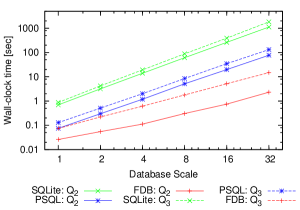
Figure 4: The effect of dataset scale on performance.

5.2 Greedy Heuristic

The size of the space of all f-plans is exponential in the size of the query, and searching for the optimal f-plan becomes impractical even for simple queries. We propose a polynomial-time greedy heuristic algorithm for finding an f-plan for a given query $Q$ and input f-tree $\mathcal{T}_{0}$:

Repeat

1. If there are any permissible selection operators, choose one involving a highest-placed node in the f-tree and execute it.

2. Else if there are any permissible aggregate operators $\gamma_{F(U)}$, choose one with maximal $\mathcal{U}$ and execute it.

3. Else if there still exists a condition $A_{i}=B_{i}$ such that $A_{i}$ and $B_{i}$ are not in the same node, calculate the cost for repeatedly pushing up (a) $A_{i}$, or (b) $B_{i}$, or (c) both $A_{i}$ and $B_{i}$, until $A_{i}$ and $B_{i}$ are siblings or one is an ancestor of the other. Pick the cheapest option and execute it.

4. Else if there is an attribute $A\in G$ with parent $B\notin G$, swap $A$ with $B$.

5. Else if there is an attribute $A\in L$ with parent $B$ such that $B$ is not before $A$ in $L$, swap $A$ with $B$,

6. Else break.

After this algorithm terminates, all selection conditions have been evaluated in (1) possibly using the restructuring from (3), all attributes not in $G$ have been aggregated in (2) possibly using the restructuring in (4), and the order condition is met because of (5). There may still be several aggregate attributes in the f-tree, the value of the final aggregate is the product (or min or max, depending on the aggregation function $F$) of these values. This can be calculated during enumeration.

If we require the result of the aggregate in a single attribute, we need to arrange all nodes dependent on the aggregation attributes into a single path. This can be achieved by repeatedly swapping them up:

1. Let $P$ be the least common ancestor in $\mathcal{T}$ of all attributes of $\mathcal{T}\setminus G$. While $P$ has a child with an atomic attribute $R$, swap $P$ and $R$.

6 Experimental Evaluation

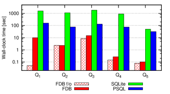
Figure 5: Performance of AGG queries on the (factorised) materialised view $R_{1}$ at scale 32.

We evaluate the performance of our query engine FDB against the SQLite and PostgreSQL open-source relational engines. Our main finding is that FDB outperforms relational engines if its input is factorised. In addition to the gain brought by factorisations, two optimisations supported by FDB are particularly important: (1) Partial aggregation that reduces the size of intermediate factorisations and (2) the reuse of existing sorting orders as enabled by local, partial restructuring of factorisations. While the former optimisation is relevant to queries with aggregates, the second is essential to queries with order-by clauses and can make a difference even for simple queries that just sort the input relation. We also found that limit clauses, which allow users to ask for the first $k$ tuples in the result, can benefit from factorisations coupled with partial restructuring.

Competing Engines. FDB is implemented in C++ for execution in main memory. We consider two flavours in the experiments: FDB produces flat, relational output, whereas FDB f/o produces factorised output. The lightweight query engine SQLite 3.7.7 was tuned for main memory operation by turning off the journal mode and synchronisations and by instructing it to use in-memory temporary store. Similarly, we run PostgreSQL 9.1.8 (PSQL) with the following parameters: fsync, synchronous commit, full page writes and background writer are off, shared buffers, working memory and effective cache size increased to 12 GB. For PSQL we run each query three times and time the last repetition, for which internal tables are cached and queries are optimised for main memory. For all engines we report wall-clock times to execute the query plans; these times exclude importing the data from files on disk and writing the result to disk. Our measurements indicate that the disk I/O for SQLite is zero and zero or negligible for PSQL (always smaller than when reading input and writing output to disk, which increases execution time by at most 10%.)

Experimental Setup. All experiments were performed on an Intel(R) Xeon(R) X5650 dual 2.67GHz/64bit/59GB running VMWare VM with Linux 3.0.0/gcc4.6.1.

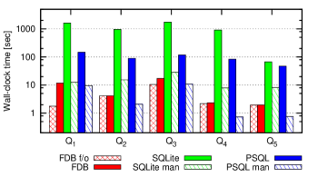
Figure 6: Performance of AGG queries on flat input at scale 32. SQLite and PSQL using their own plans and also manually optimised plans (man).

Experimental Design. We use a synthetic dataset that consists of three relations: Orders, Items, Packages, generalising the pizzeria database from Example 1. We control their sizes, and therefore the succinctness gap between factorised and flat results of queries on this dataset, using a scale parameter $s$. The number of dates on which orders are placed is $800s$, the average number of order dates per customer is $80s$ and the average number of orders per order date is 2, both with a binomial distribution. There are $100\sqrt{s}$ different items and $40\sqrt{s}$ packages of $20\sqrt{s}$ items in average. Scaling generates database instances for which the size of the natural join of all three relations grows as $s^{4}$ while its factorisation over the following f-tree $\mathcal{T}$ grows as $s^{3}$.

$$\psset{levelsep=5mm,nodesep=2.0pt,treesep=5mm}\pstree{\TR{\mbox{package}}}{\pstree{\TR{\mbox{date}}}{\TR{\mbox{customer}}}\pstree{\TR{\mbox{item}}}{\TR{\mbox{price}}}}$$

For the scale factor 32, the join has 280M tuples (1.4G singletons), while the factorisation has 4.2M singletons.

We use three sets of queries, cf. Figure 3. The set AGG consists of five queries with aggregates and group-by clauses. The set AGG+ORD consists of four queries with order-by clauses and aggregates. The set ORD consists of four order-by queries on top of sorted relations $R_{2}$ and $R_{3}$.

We next present five experiments whose focus is on performance of query evaluation; a comprehensive experimental evaluation of our query optimisation techniques is available online at the FDB web page: http://www.cs.ox.ac.uk/projects/FDB/. For all queries used in the following experiments, the heuristic algorithm gives optimal f-plans under the asymptotic bounds metric.

Experiment 1: Aggregate queries on materialised views. Figure 4 shows that FDB clearly outperforms SQLite and PSQL in our experiments on the factorised materialised view with AGG queries $Q_{2}$ and $Q_{3}$. The evaluation of both queries in FDB is done using partial aggregation and restructuring, similar to the query $P$ in the introduction. The relational engines only perform grouping and aggregation on the materialised view; PSQL uses hashing while SQLite uses sorting to implement grouping. The performance gap widens as we increase the scale factor and raises from one order of magnitude for scale 1 to two orders of magnitude for scale 32 when compared to PSQL; SQLite shows one additional order of magnitude gap. Notably, the reported timing for FDB includes the enumeration of result tuples, i.e., its output is flat as for relational engines.

Figure 5 looks closer at this scenario for scale 32 and AGG queries. When computing the result as factorised data, the performance gap further widens by two orders of magnitude for $Q_{1}$. This is the time needed to enumerate the tuples in the query result and is directly impacted by the cardinality of the result. The result of $Q_{1}$ is large as it consists of all joinable triples of packages, dates, and customers. The results of the other queries have less attributes and smaller sizes. For them, the enumeration time takes comparable or much less time as computing the factorised result.

Experiment 2: Aggregate queries on relational data. Figure 6 presents FDB’s performance for evaluating aggregate queries on flat, relational data (no materialised view this time) and producing flat output. Surprisingly, FDB outperforms SQLite and PSQL in their domain. A closer look revealed that both relational engines do not use partial aggregation and hence only consider sub-optimal query plans. With handcrafted plans that make use of partial and eager aggregation [31], all engines perform similarly. If we set for factorised output, then FDB f/o outperforms FDB in case of large factorisable results ($Q_{1},Q_{3}$); for small results, there is no difference to FDB as expected.

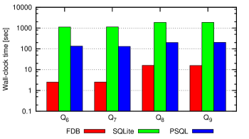
Figure 7: Performance of AGG+ORD queries on the (factorised) materialised view $R_{1}$ at scale 32.

Experiment 3: Aggregate and order-by queries on materialised views. Figure 7 shows that ordering only adds a small overhead to queries with aggregates. For FDB, the result of $Q_{2}$ is already ordered by customer, and thus the additional order-by clause in $Q_{6}$ is simply ignored by FDB. Re-ordering by the result of aggregation, as done in $Q_{7}$, does only add a marginal overhead, not visible in the plot due to the log scale on the y axis. This is explained by the relatively small result of $Q_{2}$. A similar situation is witnessed for the pair of queries $Q_{8}$ and $Q_{9}$ that apply different orders on the result to $Q_{3}$. Overall, it takes longer since $Q_{3}$ has a larger result than $Q_{2}$ (there are more pairs of date and package than customers). Following the pattern for queries $Q_{2}$ and $Q_{3}$ discussed in Experiment 1 and the lack of impact of ordering in this experiment, FDB outperforms the relational engines in this experiment, too.

Experiment 4: Partial sorting via restructuring of factorisations. In this experiment we investigate the performance of the class ORD of order-by queries, and their versions asking for the first 10 tuples only, see Figure 8. FDB restructures the factorisation whenever necessary before enumeration in the required order. The time required for the restructuring is essentially captured by the execution time of the limit variant, since enumerating the first 10 tuples only adds a small constant overhead.

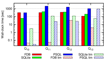
Figure 8: Performance of ORD queries with and without a LIMIT 10 statement (lim) on the (factorised) materialised view $R_{1}$ at scale 16.

Query $Q_{10}$ asks for a specific order on the materialised view $R_{2}$ that is already sorted in that order. FDB thus needs no restructuring of the view and enumerates the results. The relational engines need no additional sorting and only scan the relation $R_{1}$. This allows us to see how relation scanning compares against FDB enumeration: The latter is about the same speed as the PSQL scan. SQLite is faster than both; this is possibly because FDB is not optimised for string manipulation (by, e.g., hashing all strings in a relation). Returning the first 10 tuples only takes negligible time for both FDB and PSQL, SQLite takes longer.

Query $Q_{11}$ asks for a slightly different order than the one existing in the relational input $R_{2}$. FDB need not do any work, since its factorisation of $R_{2}$ does already support this new order, as well as the original order. Simultaneous support for several orders is a key feature of FDB. The f-tree of the factorised materialised view $R_{1}$ is $\mathcal{T}_{1}$ from the introduction, where we have package instead of pizza. It can therefore support both orders (package, date, item) and (package, item, date). In contrast, both relational engines need to sort the relation from scratch. Enumeration with FDB takes the same time as for $Q_{10}$, yet now the relational engines need more time to sort, PSQL about one order of magnitude more. Even to return the first 10 tuples requires major work for the relational engines, while FDB returns each of these tuples with constant delay and no precomputation.

Query $Q_{12}$ asks for an order that is not already supported by the f-tree of the factorised materialised view. In this case, FDB needs restructuring before the enumeration: one swap between date and its parent node package is enough, and is still faster than sorting from scratch using either of the relational engines. Returning the first 10 tuples in the required order using PSQL takes the same time as the swap.

Query $Q_{13}$ just sorts the relation $R_{3}$. Remarkably, even for sorting a (non-factorised) relation, FDB outperforms the relational engines since it only needs to partially re-sort the input. This is achieved by swapping the attributes date and customer. The factorisation constructed by FDB groups the relation by the first attribute in the sorting order, then by the second, and so on. The swap of date and customer re-groups by customer instead of date, yet the list of packages for each date and customer remains sorted.

Experiment 5: Overhead of relational engines. PSQL and SQLite are full-fledged engines while FDB is not. To understand their overhead, we also benchmarked a basic main-memory relational engine called RDB; this has been previously used for benchmarking against FDB [5] for select-project-join queries and we extended it with sorting and aggregation operators for our purpose. We ran all queries in the previous experiments also with RDB. Where grouping is required, RDB first sorts the records (using C++ STL sort) and then performs aggregation in one scan. We found that RDB’s performance is very close to SQLite’s (which implements grouping by sorting using B-trees) and we therefore not explicitly show it in the plots.

7 Related Work

There is a wealth of related work on storage layout, succinct data representations, schema design, polynomial-delay enumeration for query results, and aggregate processing.

Storage layout. Similar to FDB, columnar stores, e.g., MonetDB [7] and C-Store [7, 29], target read-optimised scenarios. Horizontal partitioning or sharding is used for data distribution and can increase parallelisation of query processing. Partitioning-based automated physical database design [3, 14] has been proposed for maximising the performance of a particular workload. RodentStore is an adaptive and declarative storage system providing a high-level interface for describing the physical representation of data [9]. In contrast to existing approaches, FDB intertwines vertical and horizontal partitioning of relational data. For this reason, existing techniques are not directly applicable.

Data compression. Data compression shares with factorisation the goal of compact data representation, as used e.g., for column compression [29, 14] and dictionary-based value compression in Oracle [24]. Such data compression schemes can benefit FDB and complement the structural compression brought by factorised representations.

Schema design. Factorisation trees rely on join dependencies, which form the basis of the fifth normal form [25]. Join dependencies were not used previously as a basis for a representation system for relational data that can support query processing. Factorisations can go beyond the class of factorisation trees and the query processing techniques developed in this paper can be adapted to more general factorisations.

Succinct representation systems and applications. Factorised databases have been introduced recently [22, 5]. Generalised hierarchical decompositions [10] and compacted relations [6] are equivalent to factorisations over f-trees but questions of succinctness have not been addressed by earlier work. Nested relations [18, 16, 1] are also structurally equivalent to factorisations over f-trees, their data model is explicitly non-first normal form. Previous work does not study representing standard relations by nested relations, nor the related questions of choosing a succinct representation and evaluating queries on the represented relation.

In provenance and probabilistic databases, factorisations can be used for compact encoding of provenance polynomials [12, 21] and for efficient query evaluation [30]. They can be used to represent large spaces of possibilities or choices in design specification [15] and in incomplete information [20].

Aggregate processing. Our approach to partial aggregation before restructuring is intimately related to work by Yan and Larson on partially pushing $sum$ and $count$ aggregation past joins  [31]. This is called eager aggregation and contrasts with lazy aggregation, which is applied after joins. While their technique relies on query rewriting, our approach conveys information about partial aggregation in the f-trees of temporary results, and replaces elaborate rewrite rules by simple compositional rules for aggregation operators. In relational processing, eager aggregation reduces the size of relations participating in a join and prevents unnecessary computation of combinations of values that are later aggregated anyway. FDB already avoids the explicit enumeration of such combinations by means of factorisation, whose size is at most the size of the join input and much less for selective joins. FDB thus combines the advantages of both lazy and eager aggregation.

Enumeration of query results. Factorised representations of query results allow for constant-delay enumeration of tuples. For more succinct representations, e.g., binary join decompositions [11] or just the pair of the query and the database [4], retrieving any tuple in the query result is NP-hard. Factorised representations can thus be seen as compilations of query results that allow for efficient subsequent processing. There has been no previous work on enumeration in sorted order on factorised data. The closest in spirit to ours is on polynomial-delay enumeration in sorted order for results to acyclic conjunctive queries [17].

8 Conclusion and Future Work

In this paper we introduce processing techniques for queries with aggregates and order-by clauses in factorised databases. These techniques include partial aggregation and constant-delay enumeration for query results and are implemented in the main-memory query engine called FDB. We show experimentally that FDB can outperform the open-source engines SQLite and PostgreSQL if its input is represented by views materialised as factorisations.

An intriguing research direction is to go beyond factorisations defined by f-trees and consider more succinct representations such as decision diagrams.

References

- [1] S. Abiteboul and N. Bidoit. Non first normal form relations: An algebra allowing data restructuring. JCSS, 33(3):361–393, 1986.
- [2] S. Abiteboul, R. Hull, and V. Vianu. Foundations of Databases. Addison-Wesley, 1995.
- [3] S. Agrawal, V. Narasayya, and B. Yang. Integrating vertical and horizontal partitioning into automated physical database design. In SIGMOD, pages 359–370, 2004.
- [4] G. Bagan, A. Durand, and E. Grandjean. On acyclic conjunctive queries and constant delay enumeration. In CSL, pages 208–222, 2007.
- [5] N. Bakibayev, D. Olteanu, and J. Závodný. FDB: A query engine for factorised relational databases. PVLDB, 5(11):1232–1243, 2012.
- [6] F. Bancilhon, P. Richard, and M. Scholl. On line processing of compacted relations. In VLDB, pages 263–269, 1982.
- [7] P. A. Boncz, S. Manegold, and M. L. Kersten. Database architecture optimized for the new bottleneck: Memory access. In VLDB, pages 54–65, 1999.
- [8] R. K. Brayton. Factoring logic functions. IBM J. Res. Develop., 31(2):187–198, 1987.
- [9] P. Cudré-Mauroux, E. Wu, and S. Madden. The case for RodentStore: An adaptive, declarative storage system. In CIDR, 2009.
- [10] C. Delobel. Normalization and hierarchical dependencies in the relational data model. TODS, 3(3):201–222, 1978.
- [11] G. Gottlob. On minimal constraint networks. In CP, pages 325–339, 2011.
- [12] T. J. Green, G. Karvounarakis, and V. Tannen. Provenance semirings. In PODS, pages 31–40, 2007.
- [13] M. Grohe and D. Marx. Constraint solving via fractional edge covers. In SODA, pages 289–298, 2006.
- [14] M. Grund, J. Krüger, H. Plattner, A. Zeier, P. Cudré-Mauroux, and S. Madden. HYRISE - A main memory hybrid storage engine. PVLDB, 4(2):105–116, 2010.
- [15] T. Imielinski, S. Naqvi, and K. Vadaparty. Incomplete objects — a data model for design and planning applications. In SIGMOD, pages 288–297, 1991.
- [16] G. Jaeschke and H. J. Schek. Remarks on the algebra of non first normal form relations. In PODS, pages 124–138, 1982.
- [17] B. Kimelfeld and Y. Sagiv. Incrementally computing ordered answers of acyclic conjunctive queries. In NGITS, pages 141–152, 2006.
- [18] A. Makinouchi. A consideration on normal form of not-necessarily-normalized relation in the relational data model. In VLDB, pages 447–453, 1977.
- [19] D. Olteanu and J. Huang. Using OBDDs for efficient query evaluation on probabilistic databases. In SUM, pages 326–340, 2008.
- [20] D. Olteanu, C. Koch, and L. Antova. World-set decompositions: Expressiveness and efficient algorithms. TCS, 403(2-3):265–284, 2008.
- [21] D. Olteanu and J. Závodný. On factorisation of provenance polynomials. In TaPP, 2011.
- [22] D. Olteanu and J. Závodný. Factorised representations of query results: Size bounds and readability. In ICDT, pages 285–298, 2012.
- [23] J. Pearl. Probabilistic reasoning in intelligent systems: Networks of plausible inference. Morgan Kaufmann, 1989.
- [24] M. Pöss and D. Potapov. Data compression in Oracle. In VLDB, pages 937–947, 2003.
- [25] R. Ramakrishnan and J. Gehrke. Database management systems. McGraw-Hill, 2003.
- [26] S. Rendle. Scaling factorization machines to relational data. PVLDB, 2013. to appear.
- [27] P. Sen, A. Deshpande, and L. Getoor. Read-once functions and query evaluation in probabilistic databases. PVLDB, 3(1):1068–1079, 2010.
- [28] Simons Institute for the Theory of Computing, UC Berkeley. Workshop on ”Succinct Data Representations and Applications”, September 2013. http://simons.berkeley.edu/workshop_bigdata1.html.
- [29] M. Stonebraker, D. J. Abadi, A. Batkin, X. Chen, M. Cherniack, M. Ferreira, E. Lau, A. Lin, S. Madden, E. J. O’Neil, P. E. O’Neil, A. Rasin, N. Tran, and S. B. Zdonik. C-Store: A Column-oriented DBMS. In VLDB, pages 553–564, 2005.
- [30] D. Suciu, D. Olteanu, C. Ré, and C. Koch. Probabilistic databases. Synthesis Lectures on Data Management. Morgan & Claypool Publishers, 2011.
- [31] W. P. Yan and P.-Å. Larson. Eager aggregation and lazy aggregation. In VLDB, pages 345–357, 1995.