Stochastic Optimization of PCA with Capped MSG

Abstract

We study PCA as a stochastic optimization problem and propose a novel stochastic approximation algorithm which we refer to as “Matrix Stochastic Gradient” (MSG), as well as a practical variant, Capped MSG. We study the method both theoretically and empirically.

1 Introduction

Principal Component Analysis (PCA) is a ubiquitous tool used in many data analysis, machine learning and information retrieval applications. It is used for obtaining a lower dimensional representation of a high dimensional signal that still captures as much as possible of the original signal. Such a low dimensional representation can be useful for reducing storage and computational costs, as complexity control in learning systems, or to aid in visualization.

PCA is typically phrased as a question about a fixed data set: given a data set of $n$ vectors in $\mathbb{R}^{d}$, what is the $k$-dimensional subspace that captures most of the variance in the data set (or equivalently, that is best in reconstructing the vectors, minimizing the sum squared distances, or residuals, to the subspace)? It is well known that this subspace is given by the leading $k$ components of the singular value decomposition of the data matrix (or equivalently of the empirical second moment matrix). And so, the study of computational approaches for PCA has mostly focused on methods for finding the SVD (or leading components of the SVD) for a given $n\times d$ matrix (Oja and Karhunen, 1985; Sanger, 1989; Mitliagkas et al., 2013).

In this paper we approach PCA as a stochastic optimization problem, where the goal is to optimize a “population objective” based on i.i.d. draws from the population. That is, in the case of PCA, we consider a setting in which we have some unknown source (“population”) distribution $\mathcal{D}$ over $\mathbb{R}^{d}$, and the goal is to find the $k$-dimensional subspace maximizing the (uncentered) variance of $\mathcal{D}$ inside the subspace (or equivalently, minimizing the average squared residual in the population), based on i.i.d. samples from $\mathcal{D}$. The main point here is that the true objective is not how well the subspace captures the sample (i.e. the “training error”), but rather how well the subspace captures the underlying source distribution (i.e. the “generalization error”). Furthermore, we are not concerned here with capturing some “true” subspace, and so do not measure the angle to it, but rather at finding a “good” subspace, that is almost as good as the optimal one.

Of course, finding the subspace that best captures the sample is a very reasonable approach to PCA on the population. This is essentially an Empirical Risk Minimization (ERM) approach. However, when comparing it to alternative, perhaps computationally cheaper, approaches, we argue that one should not compare the error on the sample, but rather the population objective. Such a view can justify and favor computational approaches that are far from optimal on the sample, but are essentially as good as ERM on the population.

Such a population-based view of optimization has recently been advocated in machine learning, and has been used to argue for crude stochastic approximation approaches (online-type methods) over sophisticated deterministic optimization of the empirical (training) objective (i.e. “batch” methods)  (Bottou and Bousquet, 2007; Shalev-Shwartz and Srebro, 2008). A similar argument was also made in the context of stochastic optimization, where Nemirovski et al. (2009) argues for stochastic approximation (SA) approaches over ERM. Accordingly, SA approaches, mostly variants of Stochastic Gradient Descent, are often the methods of choice for many learning problems, especially when very large data sets are available (Shalev-Shwartz et al., 2007; Collins et al., 2008; Shalev-Shwartz and Tewari, 2009). We would like to take the same view in order to advocate for, study, and develop stochastic approximation approaches for PCA.

In an empirical study of stochastic approximation methods for PCA, a heuristic “incremental” method showed very good empirical performance (Arora et al., 2012). However, no theoretical guarantees or justification were given for incremental PCA. In fact, it was shown that for some distributions it can converge to a suboptimal solution with high probability (see Section 5.2 for more about this “incremental” algorithm). Also relevant is careful theoretical work on online PCA by Warmuth and Kuzmin (2008), in which an online regret guarantee was established. Using an online-to-batch conversion, this online algorithm can be converted to a stochastic approximation algorithm with good iteration complexity, however the runtime for each iteration is essentially the same as that of ERM (i.e. of PCA on the sample), and thus senseless as a stochastic approximation method (see Section 3.3 for more on this algorithm).

In this paper we borrow from these two approaches and present a novel algorithm for stochastic PCA—the Matrix Stochastic Gradient (MSG) algorithm. MSG enjoys similar iteration complexity to Warmuth’s and Kuzmin’s algorithm, and in fact we present a unified view of both algorithms as different instantiations of Mirror Descent for the same convex relaxation of PCA. We then present the capped MSG, which is a more practical variant of MSG, has very similar updates to those of the “incremental” method, and works well in practice, and does not get stuck like the “incremental” method. The Capped MSG is thus a clean, theoretically well founded method, with interesting connections to other stochastic/online PCA methods, and excellent practical performance—a “best of both worlds” algorithm.

2 Problem Setup

We consider PCA as the problem of finding the maximal (uncentered) variance $k$-dimensional subspace with respect to an (unknown) distribution $\mathcal{D}$ over $x\in\mathbb{R}^{d}$. We assume without loss of generality a scaling such that $\mathbb{E}_{x\sim\mathcal{D}}[\left\lVert{x}\right\rVert^{2}]\leq 1$. We also require for our analysis a bounded fourth moment: $\mathbb{E}_{x\sim\mathcal{D}}[\left\lVert{x}\right\rVert^{4}]\leq 1$. We represent a $k$-dimensional subspace by an orthonormal basis, collected in the columns of a matrix $U$. With this parametrization, PCA is defined as the following stochastic optimization problem,

$$\mbox{maximize}: \ \ \mathbb{E}_{x\sim\mathcal{D}}[x^{T}UU^{T}x]$$ (2.1)

$$\mbox{subject to}: \ \ U\in\mathbb{R}^{d\times k},U^{T}U=I.$$

In a stochastic optimization setting we do not have direct knowledge of the distribution and have access to it only through i.i.d. samples—these can be thought of as “training examples”. As with other studies of stochastic approximation methods, we are less concerned with the number of required samples, but rather with the overall runtime required to obtain an $\epsilon$-suboptimal solution.

The standard approach to (2.1) is empirical risk minimization (ERM): given samples $\{x_{t}\}_{t=1}^{T}$, from the distribution, we compute the empirical covariance matrix ${\hat{C}=\frac{1}{T}\sum_{t=1}^{T}x_{t}x_{t}^{T}}$, and pick the columns of $U$ to be the eigenvectors of $\hat{C}$ corresponding to the top-$k$ eigenvalues. This approach requires $O(d^{2})$ memory and $O(d^{2})$ operations just in order to compute the covariance matrix, plus some additional time for the SVD. We are interested in methods with much lower sample time and space complexity, preferably linear rather than quadratic in $d$.

3 MSG and MEG

A natural stochastic approximation (SA) approach to PCA is to perform projected stochastic gradient descent (SGD) on Problem 2.1, with respect to the variable $U$. This leads to the stochastic power method with each iteration given as

$$U^{(t+1)}=\mathcal{P}_{orth}\left(U^{(t)}+\eta x_{t}x_{t}^{T}\right),$$

where, $x_{t}x_{t}^{T}$ is the gradient of the PCA objective w.r.t. $U$, $\eta$ is a step size, and $\mathcal{P}_{orth}\left(\cdot\right)$ projects its argument onto the set of orthogonal matrices. Unfortunately, although SGD is well understood for convex problems, Problem 2.1 is non-convex. Consequently, obtaining a theoretical understanding of the stochastic power method, or of how the step size should be set, has proved elusive. Under some conditions, convergence to the optimal solution can be ensured, but no rate is known (Oja and Karhunen, 1985; Sanger, 1989; Arora et al., 2012).

Instead, we consider a re-parameterization of the PCA problem where the objective is convex. Instead of representing a linear subspace in terms of its basis matrix, $U$, we parametrize it using the corresponding projection matrix $M=UU^{T}$. We can now reformulate the PCA problem as

$$\mbox{maximize}: \ \ \mathbb{E}_{x\sim\mathcal{D}}[x^{T}Mx]$$ (3.1)

$$\mbox{subject to}: \ \ M\in\mathbb{R}^{d\times d},\sigma_{i}\left({M}\right)\in\left\{0,1\right\},\operatorname{rank}M=k,$$

where $\sigma_{i}\left({M}\right)$ is the $i^{th}$ eigenvalue of $M$.

We now have a convex (even linear) objective, but the constraints in (3.1) are not convex. This prompts us to consider its convex relaxation:

$$\mbox{maximize}: \ \ \mathbb{E}_{x\sim\mathcal{D}}[x^{T}Mx]$$ (3.2)

$$\mbox{subject to}: \ \ M\in\mathbb{R}^{d\times d},0\preceq M\preceq I,\operatorname{tr}M=k.\quad\quad\ \ \ \ \$$

Since the objective is linear, and the constraint set of (3.2) is just the convex hull of the constraints of (3.1), an optimum of (3.2) is always attained at a “vertex”, i.e. a point on the boundary of the original constraints (3.1). The optimum of (3.1) and (3.2) are thus the same (strictly speaking—every optimum of (3.1) is also an optimum of (3.2)), and solving (3.2) is equivalent to solving (3.1).

Furthermore, even if some $\epsilon$-suboptimal solution we find for (3.2) is not rank-$k$, i.e. is not a feasible point of (3.1), we can easily sample from it a rank-$k$ solution, feasible for (3.1), with the same value (in expectation). This follows from the following result of Warmuth and Kuzmin (2008).

Lemma 3.1 (Rounding (Warmuth and Kuzmin, 2008)).

Any feasible solution of (3.2) can be expressed as a convex combination of at most $d$ feasible solutions of (3.1).

Furthermore, Algorithm 4.1 of Warmuth and Kuzmin (2008) shows how to efficiently find such a convex combination. Since the objective is linear, treating the coefficients of the convex combination as sampling weights and choosing randomly among the $d$ components yields a rank-$k$ matrix with the desired objective function value, in expectation.

3.1 Matrix Stochastic Gradient

Performing SGD on the convex Problem 3.2 (w.r.t. the variable $M$) yields the following iterates:

$$M^{(t+1)}=\mathcal{P}\left(M^{(t)}+\eta x_{t}x_{t}^{T}\right),$$ (3.3)

where the projection is now performed onto the (convex) constraints of (3.2). The Matrix Stochastic Gradient (MSG) algorithm entails:

1. Choose step-size $\eta$, iteration count $T$, and starting point $M^{(0)}$.

2. Iterate the updates (3.3) $T$ times, each time using an independent sample $x_{t}\sim\mathcal{D}$.

3. Average the iterates as $\bar{M}=\frac{1}{T}\sum_{t=1}^{T}M^{(t)}$.

4. Sample a rank-$k$ solution $\tilde{M}$ from $\bar{M}$ using the rounding procedure discussed in the previous section.

Analyzing MSG is straightforward using the standard SGD analysis (Nemirovski and Yudin, 1983):

Theorem 1.

After $T$ iterations of MSG (on Problem 3.2), with step size $\eta=\sqrt{\frac{k}{T}}$, and starting at $M^{(0)}=0$,

$$\mathbb{E}[\mathbb{E}_{x\sim\mathcal{D}}[x^{T}\tilde{M}x]]\geq\mathbb{E}_{x\sim\mathcal{D}}[x^{T}M^{*}x]-\frac{1}{2}\sqrt{\frac{k}{T},}$$

where the expectation is w.r.t. the i.i.d. samples $x_{1},\ldots,x_{T}\sim\mathcal{D}$ and the rounding, and $M^{*}$ is the optimum of (3.1).

Proof.

Standard SGD analysis of Nemirovski and Yudin (1983) yields that

$$\mathbb{E}[x^{T}M^{*}x-x^{T}\bar{M}x]\leq\frac{\eta}{2}\mathbb{E}_{x\sim\mathcal{D}}[\|g\|^{2}_{F}]+\frac{\|M^{*}-M^{(0)}\|^{2}_{F}}{2\eta T},$$ (3.4)

where $g=xx^{T}$ is the gradient of the PCA objective. Now, $\mathbb{E}_{x\sim\mathcal{D}}[\|g\|^{2}_{F}]=\mathbb{E}_{x\sim\mathcal{D}}[\|x\|^{4}]\leq 1$ and $\left\lVert{M^{*}-M^{(0)}}\right\rVert_{F}^{2}=\left\lVert{M^{*}}\right\rVert_{F}^{2}=k$. In the last inequality, we used the fact that $M^{*}$ has $k$ eigenvalues of value $1$ each, and hence $\left\lVert{M^{*}}\right\rVert_{F}=\sqrt{k}$. ∎

3.2 Efficient Implementation and Projection

$\mbox{{msg-step}}\left(d,k,m:\mathbb{N},U^{\prime}:\mathbb{R}^{d\times m},\sigma^{\prime}:\mathbb{R}^{m},x:\mathbb{R}^{d},\eta:\mathbb{R}\right)$
1	$\hat{x}\leftarrow\sqrt{\eta}(U^{\prime})^{T}x$; $x_{\perp}\leftarrow\sqrt{\eta}x-U^{\prime}\hat{x}$; $r\leftarrow\left\lVert{x_{\perp}}\right\rVert$;
2	$\mbox{{if }}r>0$
3		$V,\sigma\leftarrow\mbox{{eig}}([\mbox{{diag}}(\sigma^{\prime})+\hat{x}\hat{x}^{T},r\hat{x};r\hat{x}^{T},r^{2}])$;
4		$U\leftarrow[U^{\prime},x_{\perp}/r]V$;
5	else
6		$V,\sigma\leftarrow\mbox{{eig}}(\mbox{{diag}}(\sigma^{\prime})+\hat{x}\hat{x}^{T})$;
7		$U\leftarrow U^{\prime}V$;
8	$\sigma\leftarrow$ distinct eigenvalues in $\sigma$; $\kappa\leftarrow$ corresponding multiplicities;
9	$\sigma\leftarrow$ project $(d,k,m,\sigma,\kappa)$;
10	$\mbox{{return }}U,\sigma$;

Algorithm 1 Matrix stochastic gradient (MSG) update: compute an eigendecomposition of $M^{\prime}+\eta xx^{T}$ from a rank-$n$ eigendecomposition $M^{\prime}=U^{\prime}\mbox{{diag}}(\sigma^{\prime})(U^{\prime})^{T}$ and project the resulting solution onto the constraint set. The computational cost of this algorithm is dominated by the matrix multiplication defining $U$ (line $4$ or $7$) costing $O(m^{2}d)$ operations.

A naive implementation of the MSG update requires $O(d^{2})$ memory and $O(d^{2})$ operations per iteration. In this section, we show how to perform this update efficiently by maintaining an up-to-date eigendecomposition of $M^{(t)}$. Pseudo-code for the update is given as Algorithm 1. Consider the eigendecomposition $M^{(t)}=U^{\prime}\mbox{{diag}}(\sigma)(U^{\prime})^{T}$, at the $t^{th}$ iteration, where $\operatorname{rank}(M^{(t)})=k_{t}$ and $U^{\prime}\in\mathbb{R}^{d\times k_{t}}$. Given a new observation $x_{t}$, the eigendecomposition of $M^{(t)}+\eta x_{t}x_{t}^{T}$ can be updated efficiently using a $(k_{t}+1)\times(k_{t}+1)$ SVD (Brand, 2002; Arora et al., 2012) (steps 1-7 of Algorithm 1). This rank-one eigen-update is followed by projection onto the constraints of (3.2), invoked as project in step 8 of Algorithm 1, discussed in the following paragraphs and given as Algorithm 2. The projection procedure is based on the following lemma:

Lemma 3.2.

Let $M^{\prime}\in\mathbb{R}^{d\times d}$ be a symmetric matrix, with eigenvalues $\sigma_{1}^{\prime},\dots,\sigma_{d}^{\prime}$ and associated eigenvectors $v_{1}^{\prime},\dots,v_{d}^{\prime}$. Its projection $M=\mathcal{P}\left(M^{\prime}\right)$ onto the feasible region of Problem 3.2 with respect to the Frobenius norm, is the unique feasible matrix which has the same eigenvectors as $M^{\prime}$, with the associated eigenvalues $\sigma_{1},\dots,\sigma_{d}$ satisfying:

$$\sigma_{i}=\max\left(0,\min\left(1,\sigma_{i}^{\prime}+S\right)\right)$$

with $S\in\mathbb{R}$ being chosen in such a way that $\sum_{i=1}^{d}\sigma_{i}=k$.

Proof.

In Appendix A. ∎

This result shows that projecting onto the feasible region amounts to finding the value of $S$ such that, after shifting the eigenvalues by $S$ and clipping the results to $[0,1]$, the result is feasible. Importantly, the projection operates only on the eigenvalues. Algorithm 2 contains pseudocode which finds $S$ from a list of eigenvalues. It is optimized to efficiently handle repeated eigenvalues—rather than receiving the eigenvalues in a length-$d$ list, it instead receives a length-$n$ list containing only the distinct eigenvalues, with $\kappa$ containing the corresponding multiplicities. In Sections 4 and 5, we will see why this is an important optimization.

The central idea motivating the algorithm is that, in a sorted array of eigenvalues, all elements with indices below some threshold $i$ will be clipped to $0$, and all of those with indices above another threshold $j$ will be clipped to $1$. The pseudocode simply searches over all possible pairs of such thresholds until it finds the one that works.

The rank-one eigen-update combined with the fast projection step yields an efficient MSG update that requires $O(dk_{t})$ memory and $O(dk_{t}^{2})$ operations per iteration, where recall that $k_{t}$ is the rank of the iterate $M^{(t)}$. This is a significant improvement over the $O(d^{2})$ memory and $O(d^{2})$ computation required by a standard implementation of MSG, if the iterates have relatively low rank.

$\mbox{{project}}\left(d,k,n:\mathbb{N},\sigma^{\prime}:\mathbb{R}^{n},\kappa^{\prime}:\mathbb{N}^{n}\right)$
1	$\sigma^{\prime},\kappa^{\prime}\leftarrow\mbox{{sort}}(\sigma^{\prime},\kappa^{\prime})$;
2	$i\leftarrow 1$; $j\leftarrow 1$; $s_{i}\leftarrow 0$; $s_{j}\leftarrow 0$; $c_{i}\leftarrow 0$; $c_{j}\leftarrow 0$;
3	$\mbox{{while }}i\leq n$
4		$\mbox{{if }}(i<j)$
5			$S\leftarrow(k-(s_{j}-s_{i})-(d-c_{j}))/(c_{j}-c_{i})$;
6			$b\leftarrow($
7				$(\sigma_{i}^{\prime}+S\geq 0)\mbox{{ and }}(\sigma_{j-1}^{\prime}+S\leq 1)$
8				$\mbox{{and }}((i\leq 1)\mbox{{ or }}(\sigma_{i-1}^{\prime}+S\leq 0))$
9				$\mbox{{and }}((j\geq n)\mbox{{ or }}(\sigma_{j+1}^{\prime}\geq 1))$
10			$)$;
11			$\mbox{{return }}S\mbox{{ if }}b$;
12		$\mbox{{if }}(j\leq n)\mbox{{ and }}(\sigma_{j}^{\prime}-\sigma_{i}^{\prime}\leq 1)$
13			$s_{j}\leftarrow s_{j}+\kappa_{j}^{\prime}\sigma_{j}^{\prime}$; $c_{j}\leftarrow c_{j}+\kappa_{j}^{\prime}$; $j\leftarrow j+1$;
14		else
15			$s_{i}\leftarrow s_{i}+\kappa_{i}^{\prime}\sigma_{i}^{\prime}$; $c_{i}\leftarrow c_{i}+\kappa_{i}^{\prime}$; $i\leftarrow i+1$;
16	return error;

Algorithm 2 Routine which finds the $S$ of Lemma 3.2. It takes as parameters the dimension $d$, “target” subspace dimension $k$, and the number of distinct eigenvalues $n$ of the current iterate. The length-$n$ arrays $\sigma^{\prime}$ and $\kappa^{\prime}$ contain the distinct eigenvalues and their multiplicities, respectively, of $M^{\prime}$ (with $\sum_{i=1}^{n}\kappa_{i}^{\prime}=d$). Line $1$ sorts $\sigma^{\prime}$ and re-orders $\kappa^{\prime}$ so as to match this sorting. The loop will be run at most $2n$ times (once for each possible increment to $i$ or $j$ on lines $12$–$15$), so the computational cost is dominated by that of the sort: $O(n\log n)$.

3.3 Matrix Exponentiated Gradient

Since $M$ is constrained by its trace, and not by its Frobenius norm, it is tempting to consider mirror descent (MD) (Beck and Teboulle, 2003) instead of SGD updates for solving Problem 3.2. Recall that the Mirror Descent updates depend on a choice of “potential function” $\Psi(\cdot)$ which should be chosen according to the geometry of the feasible set and the subgradients (Srebro et al., 2011). Using the squared Frobenius norm as a potential function, i.e. $\Psi(M)=\|M\|^{2}_{F}$, yields SGD, i.e. the MSG updates (3.3). The trace-norm constraint suggests using the von Neumann entropy of the spectrum as the potential function, i.e. $\Psi_{h}(M)=\sum_{i}\lambda_{i}(M)\log\lambda_{i}(M)$ where $\lambda_{i}$ are the eigenvalues of $M$. This leads to multiplicative updates which we refer to as Matrix Exponentiated Gradient (MEG) update similar to those presented by (Warmuth and Kuzmin, 2008). In fact, Warmuth and Kuzmin’s algorithm exactly corresponds to online Mirror Descent on (3.2) with this potential function, but taking the optimization variable to be $M_{\perp}=I-M$ (with the constraints $\operatorname{tr}M_{\perp}=d-k$ and $0\preceq M_{\perp}\preceq I$). In either case, using the entropy potential, despite being well suited for the trace-geometry, does not actually lead to better dependence on $d$ or $k$, and Mirror Descent analysis again yields an excess loss of $\sqrt{k/T}$. Warmuth and Kuzmin do present an “optimistic” analysis, with a dependence on the “reconstruction error” $L^{*}=\mathbb{E}[x^{T}(I-M^{*})x]$, which yields an excess error of $O\left(\sqrt{\frac{L^{*}k\log(d/k)}{T}}+\frac{k\log(d/k)}{T}\right)$ (their logarithmic term can be avoided by a more careful analysis).

4 MSG runtime and the rank of the iterates

As we saw, MSG requires $O(k/\epsilon^{2})$ iterations to obtain an $\epsilon$-suboptimal solution and each iteration of MSG costs $O(k_{t}^{2}d)$ operations where $k_{t}$ is the rank of iterate $M^{(t)}$. This yields a total runtime of $O(\bar{k^{2}}dk/\epsilon^{2})$, where $\bar{k^{2}}=\sum_{t=1}^{T}k^{2}_{t}$. Clearly, the runtime for MSG depends critically on the rank of the iterates. If the rank of the iterates is as large as $d$, MSG achieves a runtime that is cubic in the dimensionality. On the other hand, if the rank of the iterates is $O(k)$, the runtime is linear in the dimensionality. Fortunately, in practice the ranks are typically much lower than the dimensionality. The reason for this is that MSG performs a rank-$1$ update followed by a projection onto the constraints. Since $M^{\prime}=M^{(t)}+\eta x_{t}x_{t}^{T}$ will have a larger trace than $M^{(t)}$ (i.e. $\operatorname{tr}M^{\prime}\geq k$), the projection, as is shown by Lemma 3.2, will subtract a quantity $S$ from every eigenvalue of $M^{\prime}$, clipping each to $0$ if it becomes negative. Therefore, each MSG update will increase the rank of the iterate by at most $1$, and has the potential to decrease it, perhaps significantly. It’s very difficult to theoretically quantify how the rank of the iterates will evolve over time, but we have observed empirically that the iterates do tend to have relatively low rank.

We explore this issue in greater detail experimentally, on a distribution which we expect to be difficult for MSG. To this end, we generated data from known $32$-dimensional distributions with diagonal covariance matrices $\Sigma=\mbox{{diag}}(\sigma/\left\lVert{\sigma}\right\rVert)$, where $\sigma_{i}=\tau^{-i}/\sum_{j=1}^{32}\tau^{-j}$, for $i=1,\ldots,32$ and for some $\tau>1$. Observe that $\Sigma^{(k)}$ has a smoothly-decaying set of eigenvalues and the rate of decay is controlled by $\tau$. As $\tau\to 1$, the spectrum becomes flatter resulting in distributions that present challenging test cases for MSG. We experimented with $\tau=1.1$ and $k\in\{1,2,4\}$, where $k$ is the desired subspace dimension used by each algorithm. The data is generated by sampling the $i^{th}$ standard unit basis vector $e_{i}$ with probability $\sqrt{\Sigma_{ii}}$. We refer to this as the “orthogonal distribution”, since it is a discrete distribution over $32$ orthogonal vectors.

$k_{t}^{\prime}$	Spectrum
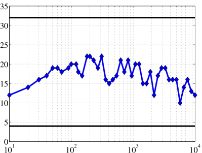
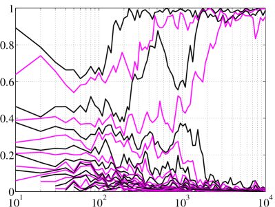
Iterations	Iterations

Figure 1: The ranks $k_{t}^{\prime}$ (left) and the eigenvalues (right) of the MSG iterates $M^{(t)}$.

In Figure 1, we show the results with $k=4$. We can see from the left-hand plot that MSG algorithm maintains a subspace of dimension around $15$. The plot on the right shows how the set of nonzero eigenvalues of the MSG iterates evolves over time, from which we can see that many of the extra dimensions are “wasted” on very small eigenvalues, corresponding to directions which leave the state matrix only a handful of iterations after they enter. This suggests that constraining $k_{t}^{\prime}$ can lead to significant speedups and motivates capped MSG updates discussed in the next section.

5 Capped MSG

While, as was observed in the previous section, MSG’s iterates will tend to have ranks $k_{t}^{\prime}$ smaller than $d$, they will nevertheless also be larger than $k$. For this reason, in practice, we recommend adding a hard constraint $K$ on the rank of the iterates:

$$\mbox{maximize}: \ \ \mathbb{E}_{x\sim\mathcal{D}}[x^{T}Mx]$$ (5.1)

$$\mbox{subject to}: \ \ M\in\mathbb{R}^{d\times d},0\preceq M\preceq I$$

$$\ \ \operatorname{tr}M=k,\operatorname{rank}M\leq K$$

We will refer MSG where the projection is replaced with a projection onto the constraints of (5.1) (i.e. where the iterates are SGD iterates on (5.1)) as “capped MSG”. For similar reasons as discussed before, as long as $K\geq k$, Problem 5.1 and Problem 3.2 have the same optimum, and it is achieved at a rank-$k$ matrix, and the extra rank constraint in 5.1 is inactive at the optimum. However, the rank constraint does affect the iterates, especially since Problem 5.1 is no longer convex. Nonetheless if $K>k$ (i.e. the hard rank-constraint $K$ is strictly larger than the target rank $k$), we can easily check if we are at a global optimum of 5.1, and hence of 3.2: if the capped MSG algorithm converges to a solution of rank $K$, then the upper bound $K$ should be increased. Conversely, if it has converged to a rank-deficient solution, then it must be the global optimum. There is thus an advantage in using $K>k$, and we recommend setting $K=k+1$, as we do in our experiments, and increasing $K$ only if a rank deficient solution is not found.

Setting $K=k$, the only way to satisfy the trace constraint is to have all non-zero eigenvalues be equal to one, and (5.1) becomes identical to (3.1). The detour through the convex problem (3.2), allows us to increase the search rank $K$, allowing for more flexibility in the search, while still encouraging the desired rank $k$ through the rank constraint.

5.1 Implementing the projection

Implementing capped MSG is similar to implementing MSG (Algorithm 1) except for the projection step. Reasoning as in the proof of Lemma 3.2 shows that if $M^{(t+1)}\!=\!\mathcal{P}\left(M^{\prime}\right)$ with $M^{\prime}=M^{(t)}+\eta x_{t}x_{t}^{T}$, then $M^{(t)}$ and $M^{\prime}$ are simultaneously diagonalizable, and therefore we can consider only how the projection acts on the eigenvalues. Hence, if we let $\sigma^{\prime}$ be the vector of the eigenvalues of $M^{\prime}$, and suppose that there are more than $K$ such eigenvalues, then there is a size-$K$ subset of $\sigma^{\prime}$ such that applying Algorithm 2 to this set gives the projected eigenvalues. Since we perform only a rank-$1$ update at every iteration, we must check at most $K$ possibilities, at a total cost of $O(K^{2}\log K)$ operations, with no effect on asymptotic runtime because Algorithm 1 requires $O(K^{2}d)$ operations.

5.2 Relationship to the incremental PCA method

The capped MSG updates with $K=k$ are similar to the incremental algorithm of Arora et al. (2012). The incremental algorithm maintains a rank-$k$ approximation of the covariance matrix with updates given by

$${M}^{(t+1)}=\mathcal{P}_{\textrm{rank-$k$}}\left({M}^{(t)}+x_{t}x_{t}^{T}\right),$$

where the projection is onto the set of rank-$k$ matrices. Unlike MSG, incremental updates do not have a step-size. Updates can be performed efficiently much in the same way as described in Section 3.2, by maintaining the eigendecomposition of the iterates.

	$k=1$	$k=2$	$k=4$
Suboptimality
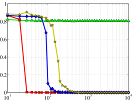
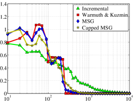
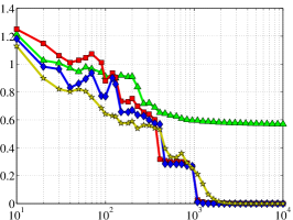
	Iterations	Iterations	Iterations

Figure 2: Comparison on simulated data for different values of parameter $k$.

The incremental algorithm was found to perform extremely well in practice–it was the best, in fact, among the compared algorithms (Arora et al., 2012). However, there exist cases in which the incremental algorithm can get stuck at a suboptimal solution. For example, If the data are drawn from a discrete distribution $\mathcal{D}$ which samples $[\sqrt{3},0]^{T}$ with probability $1/3$ and $[0,\sqrt{2}]^{T}$ with probability $2/3$, and one runs the incremental algorithm with $k=1$, then it will converge to $[1,0]^{T}$ with probability $5/9$, despite the fact that the maximal eigenvector is $[0,1]^{T}$. The reason for this failure is essentially that the orthogonality of the data interacts poorly with the low-rank projection: any update which does not entirely displace the maximal eigenvector in one iteration will be removed entirely by the projection, causing the algorithm to fail to make progress. Capped MSG algorithm with $K>k$, will not get stuck in such situations, using the additional “dimensions” to “search” in the new direction. Only as it becomes more confident in its current candidate, the trace of $M$ will become increasingly concentrated on the top $k$ directions. To illustrate this empirically, we generalized the toy example above and generated the data using the $32$-dimensional “orthogonal” distribution described in Sec. 4. This distribution presents challenging test-cases for MSG, capped MSG as well as incremental algorithm. Figure 2 shows plots of individual runs of MSG, capped MSG with $K=k+1$, the incremental algorithm, and Warmuth and Kuzmin’s algorithm, all based on the same sequence of samples drawn from the orthogonal distribution. We compare algorithms in terms of the suboptimality on the population objective based on the largest $k$ eigenvalues of the state matrix $M^{(t)}$. The plots show the incremental algorithm getting stuck for $k\in\{1,4\}$, and the others intermittently plateauing at intermediate solutions before beginning to again converge rapidly towards the optimum. This behavior is to be expected on the capped MSG algorithm, due to the fact that the dimension of the subspace stored at each iterate is constrained. However, it is somewhat surprising that MSG and Warmuth and Kuzmin’s algorithm behaved similarly, and barely faster than capped MSG.

6 Experiments

	$k=1$	$k=4$	$k=8$
Suboptimality
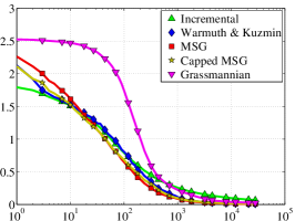
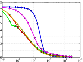
	Iterations	Iterations	Iterations
Suboptimality
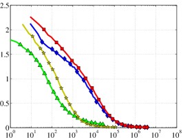
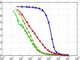
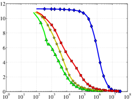
	Est. runtime	Est. runtime	Est. runtime

Figure 3: Comparison on the MNIST dataset. The top row of plots shows suboptimality as a function of iteration count, while the bottom row suboptimality as a function of estimated runtime $\sum_{s=1}^{t}(k_{s}^{\prime})^{2}$.

We also compared the algorithms on the real-world MNIST dataset, which consists of $70,000$ binary images of handwritten digits of size $28\times 28$, resulting in a dimensionality of $784$. We pre-normalized the data by mean centering the feature vectors and scaling each feature by the product of its standard deviation and the data dimension, so that each feature vector is zero mean and unit norm in expectation. In addition to MSG, capped MSG, the incremental algorithm and Warmuth and Kuzmin’s algorithm, we also compare to a Grassmannian SGD algorithm of Balzano et al. (2010). All algorithms except the incremental algorithm have a step-size parameter. In these experiments, we ran each algorithm with decreasing step sizes $\eta_{t}=c/\sqrt{t}$ for $c\in\{2^{-12},2^{-19},\ldots,2^{5}\}$ and picked the best $c$, in terms of the average suboptimality over the run, on a validation set. Since we cannot evaluate the true population objective, we estimate it by evaluating on a held-out test set. We use 40% of samples in the dataset for training, 20% for validation (tuning step-size), and 40% for testing. We are interested in learning a maximum variance subspace of dimension $k\in\{1,4,8\}$ in a single “pass” over the training sample. In order to compare MSG, capped MSG, incremental and Warmuth and Kuzmin’s algorithm in terms of runtime, we calculate the dominant term in the computational complexity: $\!\sum_{s=1}^{t}\!(k_{s}^{\prime})^{2}\!$. The results are averaged over $100$ random splits into train-validation-test sets.

We can see from Figure 3 that the incremental algorithm makes the most progress per iteration and is also the fastest of all algorithms. MSG is comparable to the incremental algorithm in terms of the the progress made per iteration. However, its runtime is slightly worse than the incremental because it will often keep a slightly larger representation (of dimension $k_{t}^{\prime}$) than the incremental algorithm. The capped MSG variant (with $K=k+1$) is significantly faster–almost as fast as the incremental algorithm, while, as we saw in the previous section, being less prone to getting stuck. Warmuth and Kuzmin’s algorithm fares well with $k=1$, but its performance drops for higher $k$. Inspection of the underlying data shows that, in the $k\in\{4,8\}$ experiments, it also tends to have a larger $k_{t}^{\prime}$ than MSG in these experiments, and therefore has a higher cost-per-iteration. Grassmannian SGD performs better than Warmuth and Kuzmin, but much worse when compared with MSG and capped MSG.

7 Conclusions

In this paper, we presented a careful development and analysis of MSG, a stochastic approximation algorithm for PCA, which enjoys good theoretical guarantees and offers a computationally efficient variant, capped MSG. We show that capped MSG is well-motivated theoretically and that it does not get stuck at a suboptimal solution. Capped MSG is also shown to have excellent empirical performance and it therefore is a much better alternative to the recently proposed incremental PCA algorithm of Arora et al. (2012). Furthermore, we provided a cleaner interpretation of PCA updates of Warmuth and Kuzmin (2008) in terms of Matrix Exponentiated Gradient (MEG) updates and showed that both MSG and MEG can be interpreted as mirror descent algorithms on the same relaxation of the PCA optimization problem but with different distance generating functions.

Appendix A Proof of Lemma 3.2

Lemma 3.2.

Let $M^{\prime}\in\mathbb{R}^{d\times d}$ be a symmetric matrix, with eigenvalues $\sigma_{1}^{\prime},\dots,\sigma_{d}^{\prime}$ and associated eigenvectors $v_{1}^{\prime},\dots,v_{d}^{\prime}$. If $M=\mathcal{P}\left(M^{\prime}\right)$ projects $M^{\prime}$ onto the feasible region of Problem 3.2 with respect to the Frobenius norm, then $M$ will be the unique feasible matrix which has the same set of eigenvectors as $M^{\prime}$, with the associated eigenvalues $\sigma_{1},\dots,\sigma_{d}$ satisfying:

$$\sigma_{i}=\max\left(0,\min\left(1,\sigma_{i}^{\prime}+S\right)\right)$$

with $S\in\mathbb{R}$ being chosen in such a way that $\displaystyle\sum_{i=1}^{d}\sigma_{i}=k$.

Proof.

The problem of finding $M$ can be written in the form of a convex optimization problem as:

$$\mbox{minimize}: \ \ \left\lVert{M-M^{\prime}}\right\rVert_{F}^{2}$$

$$\mbox{subject to}: \ \ 0\preceq M\preceq I,\operatorname{tr}M=k.$$

Because the objective is strongly convex, and the constraints are convex, this problem must have a unique solution. Letting $\sigma_{1},\dots,\sigma_{d}$ and $v_{1},\dots,v_{d}$ be the eigenvalues and associated eigenvectors of $M$, we may write the KKT first-order optimality conditions [Boyd and Vandenberghe, 2004] as:

$$0=M-M^{\prime}+\mu I-\sum_{i=1}^{d}\alpha_{i}v_{i}v_{i}^{T}+\sum_{i=1}^{d}\beta_{i}v_{i}v_{i}^{T},$$ (A.1)

where $\mu$ is the Lagrange multiplier for the constraint $\operatorname{tr}M=k$, and $\alpha_{i},\beta_{i}\geq 0$ are the Lagrange multipliers for the constraints $0\preceq M$ and $M\preceq I$, respectively. The complementary slackness conditions are that $\alpha_{i}\sigma_{i}=\beta_{i}\left(\sigma_{i}-1\right)=0$. In addition, $M$ must be feasible.

Because every term in Equation A.1 except for $M^{\prime}$ has the same set of eigenvectors as $M$, it follows that an optimal $M$ must have the same set of eigenvectors as $M^{\prime}$, so we may take $v_{i}=v_{i}^{\prime}$, and write Equation A.1 purely in terms of the eigenvalues:

$$\sigma_{i}=\sigma_{i}^{\prime}-\mu+\alpha_{i}-\beta_{i}.$$

Complementary slackness and feasibility with respect to the constraints $0\preceq M\preceq I$ gives that if $0\leq\sigma_{i}^{\prime}-\mu\leq 1$, then $\sigma_{i}=\sigma_{i}^{\prime}-\mu$. Otherwise, $\alpha_{i}$ and $\beta_{i}$ will be chosen so as to clip $\sigma_{i}$ to the active constraint:

$$\sigma_{i}=\max\left(0,\min\left(1,\sigma_{i}^{\prime}-\mu\right)\right).$$

Primal feasibility with respect to the constraint $\operatorname{tr}M=k$ gives that $\mu$ must be chosen in such a way that $\operatorname{tr}M=k$, completing the proof. ∎

References

- Arora et al. [2012] Raman Arora, Andrew Cotter, Karen Livescu, and Nathan Srebro. Stochastic optimization for pca and pls. In 50th Annual Allerton Conference on Communication, Control, and Computing, 2012.
- Balzano et al. [2010] Laura Balzano, Robert Nowak, and Benjamin Recht. Online identification and tracking of subspaces from highly incomplete information. CoRR, abs/1006.4046, 2010.
- Beck and Teboulle [2003] A. Beck and M. Teboulle. Mirror descent and nonlinear projected subgradient methods for convex optimization. Operations Research Letters, 31(3):167–175, 2003.
- Bottou and Bousquet [2007] Leon Bottou and Olivier Bousquet. The tradeoffs of large scale learning. In NIPS’07, pages 161–168, 2007.
- Boyd and Vandenberghe [2004] Stephen Boyd and Lieven Vandenberghe. Convex Optimization. Cambridge University Press, 2004.
- Brand [2002] Matthew Brand. Incremental singular value decomposition of uncertain data with missing values. In ECCV, 2002.
- Collins et al. [2008] Michael Collins, Amir Globerson, Terry Koo, Xavier Carreras, and Peter L. Bartlett. Exponentiated gradient algorithms for conditional random fields and max-margin markov networks. J. Mach. Learn. Res., 9:1775–1822, June 2008.
- Duchi et al. [2008] John Duchi, Shai Shalev-Shwartz, Yoram Singer, and Tushar Chandra. Efficient projections onto the l1-ball for learning in high dimensions. In Proceedings of the 25th international conference on Machine learning, ICML ’08, pages 272–279, New York, NY, USA, 2008. ACM.
- Mitliagkas et al. [2013] Ioannis Mitliagkas, Constantine Caramanis, and Prateek Jain. Streaming, memory-limited pca, 2013. URL http://users.ece.utexas.edu/~cmcaram/pubs/Streaming-PCA.pdf. UT-Austin.
- Nemirovski and Yudin [1983] Arkadi Nemirovski and David Yudin. Problem complexity and method efficiency in optimization. John Wiley & Sons Ltd, 1983.
- Nemirovski et al. [2009] Arkadi Nemirovski, Anatoli Juditsky, Guanghui Lan, and Alexander Shapiro. Robust stochastic approximation approach to stochastic programming. SIAM Journal on Optimization, 19(4):1574–1609, January 2009.
- Oja and Karhunen [1985] Erkki Oja and Juha Karhunen. On stochastic approximation of the eigenvectors and eigenvalues of the expectation of a random matrix. Journal of Mathematical Analysis and Applications, 106:69–84, 1985.
- Sanger [1989] Terence D. Sanger. Optimal unsupervised learning in a single-layer linear feedforward neural network. Neural Networks, 12:459–473, 1989.
- Shalev-Shwartz and Srebro [2008] Shai Shalev-Shwartz and Nathan Srebro. SVM optimization: Inverse dependence on training set size. In ICML’08, pages 928–935, 2008.
- Shalev-Shwartz and Tewari [2009] Shai Shalev-Shwartz and Ambuj Tewari. Stochastic methods for l1 regularized loss minimization. In Proceedings of the 26th Annual International Conference on Machine Learning, ICML’09, pages 929–936, New York, NY, USA, 2009. ACM.
- Shalev-Shwartz et al. [2007] Shai Shalev-Shwartz, Yoram Singer, and Nathan Srebro. Pegasos: Primal Estimated sub-GrAdient SOlver for SVM. In ICML’07, pages 807–814, 2007.
- Srebro et al. [2011] N. Srebro, K. Sridharan, and A. Tewari. On the universality of online mirror descent. Advances in Neural Information Processing Systems, 24, 2011.
- Warmuth and Kuzmin [2008] Manfred K. Warmuth and Dima Kuzmin. Randomized online PCA algorithms with regret bounds that are logarithmic in the dimension. Journal of Machine Learning Research (JMLR), 9:2287–2320, 2008.