Astronomy Letters, 2013, Vol. 39, No. 8, pp. 532–549.

Galactic Kinematics from a Sample of Young Massive Stars

V.V. Bobylev${}^{1,2},$ and A.T. Bajkova¹

¹Pulkovo Astronomical Observatory, St. Petersburg, Russia

²Sobolev Astronomical Institute, St. Petersburg State University, Russia

Abstract—Based on published sources, we have created a kinematic database on 220 massive $(>10M_{\odot})$ young Galactic star systems located within $\leq 3$ kpc of the Sun. Out of them, $\approx$100 objects are spectroscopic binary and multiple star systems whose components are massive OB stars; the remaining objects are massive Hipparcos B stars with parallax errors of no more than 10%. Based on the entire sample, we have constructed the Galactic rotation curve, determined the circular rotation velocity of the solar neighborhood around the Galactic center at $R_{0}=8$ kpc, $V_{0}=259\pm 16$ km s${}^{-1},$ and obtained the following spiral density wave parameters: the amplitudes of the radial and azimuthal velocity perturbations $f_{R}=-10.8\pm 1.2$ km s${}^{-1},$ and $f_{\theta}=7.9\pm 1.3$ km s${}^{-1},$ respectively; the pitch angle for a two-armed spiral pattern $i=-6.0^{\circ}\pm 0.4^{\circ}$, with the wavelength of the spiral density wave near the Sun being $\lambda=2.6\pm 0.2$ kpc; and the radial phase of the Sun in the spiral density wave $\chi_{\odot}=-120^{\circ}\pm 4^{\circ}$. We show that such peculiarities of the Gould Belt as the local expansion of the system, the velocity ellipsoid vertex deviation, and the significant additional rotation can be explained in terms of the density wave theory. All these effects decrease noticeably once the influence of the spiral density wave on the velocities of nearby stars has been taken into account. The influence of Gould Belt stars on the Galactic parameter estimates has also been revealed. Eliminating them from the kinematic equations has led to the following new values of the spiral density wave parameters: $f_{\theta}=2.9\pm 2.1$ km s^-1 and $\chi_{\odot}=-104^{\circ}\pm 6^{\circ}$.

INTRODUCTION

A wide variety of data are used to study the Galactic kinematics. These include the line-of-sight velocities of neutral and ionized hydrogen clouds with their distances estimated by the tangential point method (Clemens 1985; McClure-Griffiths and Dickey 2007; Levine et al. 2008), Cepheids with the distance scale based on the period–luminosity relation, open star clusters and OB associations with photometric distances (Mishurov and Zenina 1999; Rastorguev et al. 1999; Zabolotskikh et al. 2002; Bobylev et al. 2008; Mel’nik and Dambis 2009), and masers with their trigonometric parallaxes measured by VLBI (Reid et al. 2009; McMillan and Binney 2010; Bobylev and Bajkova 2010; Bajkova and Bobylev 2012). The youngest massive high luminosity (OB) stars are also of great interest, because they have not moved far away from their birthplace in their lifetime, clearly tracing the Galactic spiral structure. Such stars were used by many authors on various spatial scales to study the Galactic kinematics (Moffat et al. 1998; Avedisova 2005; Popova and Loktin 2005; Branham 2006). Among the youngest OB stars, the fraction of binary and multiple systems reaches 70–80%. However, the kinematics of precisely such systems has been studied more poorly than that of single stars.

At present, great interest in massive binaries is related to the study of the Galaxy’s spatial, kinematic, and dynamical properties. For example, it is important to know the positions of high-mass X-ray binaries in the Galaxy (Coleiro and Chaty 2012), their connection with the Galactic spiral structure (Lutovinov et al. 2005), the distribution of possible presupernovae, the progenitors of neutron stars and black holes, around the Sun (Hohle et al. 2010), the distribution of runaway OB stars (Tetzlaff et al. 2011), etc.

Binary systems usually have a long history of spectroscopic and photometric observations. Therefore, in particular, their systemic line-of-sight velocities, spectral classification, and photometry are well known. Here, we focus on revealing the binary systems containing predominantly O stars that are suitable for studying the kinematic characteristics of the solar neighborhood and the Galaxy as a whole. Among the O stars from the Hipparcos catalogue (1997), only 12 have trigonometric parallaxes differing significantly from zero and the farthest of them, 10 Lac, is only $\approx$540 pc away from the Sun (Maiz-Apellániz et al. 2008). Therefore, we use less reliable spectrophotometric distance estimates for many of the stars from our sample.

The goal of this paper is to create a kinematic database on Galactic massive $(>10M_{\odot})$ young star systems within 2–3 kpc of the Sun, to determine the main kinematic parameters of the Galaxy, including the spiral density wave parameters, using this database, to reveal runaway stars, to explain the kinematic peculiarities of the (Gould Belt) stars nearest to the Sun, and to study the influence of the latter on the Galactic parameters being determined.

1 DATA

1.1 Distances

Studying the total space velocities of stars requires knowing six quantities: the equatorial coordinates ($\alpha,\delta$), the heliocentric distance ($r$), two proper motion components ($\mu_{\alpha}\cos\delta,\mu_{\delta}$), and the line-of-sight velocity ($V_{r}$). It is important to note that the requirement of a high accuracy for the space velocities imposes a constraint on the heliocentric distances of stars, which is no more than 3 kpc in our case. For example, since $V_{t}=4.74r\mu_{t},$ where $\mu_{t}=\sqrt{\mu^{2}_{\alpha}\cos^{2}\delta+\mu^{2}_{\delta}},$ at a typical error $\sigma_{\mu_{t}}\approx 1.4$ mas yr${}^{-1},$ the contribution from the proper motion error to the total velocity of a star will be a significant fraction of the total velocity, $\sigma_{V_{t}}\approx 20$ km s${}^{-1},$ already at a distance of 3 kpc.

Our sample was produced as follows.

First of all, it includes O-type stars for which the relative error of the trigonometric parallax does not exceed $\approx$15%. Among these stars, there are also single ones. The distances corrected for the Lutz–Kelker bias were taken from Maiz-Apellániz et al. (2008).

Our sample includes five stars whose components are massive O stars with known highly accurate orbital (dynamical) parallaxes: $\theta^{1}$Ori C (Kraus et al. 2009), $\sigma$ Ori (Caballero 2008), $\gamma^{2}$Vel (North et al. 2007a), $\delta$ Sco (Tycner et al. 2011), and $\sigma$ Sco (North et al. 2007b). For four of these systems (except $\sigma$ Ori), the orbital semimajor axes were measured with ground-based optical interferometers, such as, for example, SUSI (Sydney University Stellar Interferometer).

An example of a high accuracy of the dynamical parallax is the triple system $\theta^{1}$Ori C (Sp: O+?+?; with a total mass of $44M_{\odot}$). It is one of the Orion Trapezium members for which the Hipparcos trigonometric parallax is negative. In contrast, the distance calculated from the dynamical parallax is $r=410\pm 20$ pc. This is in excellent agreement with the estimate of $418\pm 6$ pc to the region Orion–KL obtained by VLBI within the VERA program (Japan) using the maser SiO emission at 43.122 GHz (Kim et al. 2008). For the remaining six systems from this list $\sigma$ Ori (O9.5+B0.5; $20M_{\odot}+12M_{\odot}$), $\gamma^{2}$Vel (O+WR; $29M_{\odot}+9M_{\odot}$), $\delta$ Sco (B1+B1; $12M_{\odot}+7M_{\odot}$), $\sigma$ Sco (B0+B1; $18M_{\odot}+12M_{\odot}$), $\beta$ Cen (B1+B1; $11M_{\odot}+10M_{\odot}$), $\lambda$ Sco (B1.5+B2+PMS; $10M_{\odot}+8M_{\odot}$+?), the situation is less dramatic—their dynamical parallaxes have smaller errors (the trigonometric distances were improved by analyzing the orbits). The distances calculated using the dynamical parallaxes for $\beta$ Cen and $\lambda$ Sco make them twice as close compared to the trigonometric estimates (Ausseloos et al. 2006; Tango et al. 2006).

Among the visual binary stars in our sample, there are two massive triple systems, $\beta$ Cep (WDS J21287+7034) and $\gamma$ Lup (WDS J15351–4110), with known estimates of their orbital parallaxes (Docobo and Andrade 2006) that are as accurate as the trigonometric measurements. Significantly, for example, for $\gamma$ Lup (B1+B2+B3; 12M_⊙+8M_⊙+7M_⊙), the dynamical parallax $\pi_{f}=6.6\pm 0.4$ mas was estimated at the then available trigonometric parallax estimate $\pi_{tr}=5.75\pm 1.24$ mas (Hipparcos 1997). In contrast, the trigonometric parallax from the revised version of Hipparcos is $\pi_{tr}=7.75\pm 0.50$ mas (van Leeuwen 2007); it became larger in agreement with the analysis of the stellar orbits. Similarly, for $\beta$ Cep (B3+A7+A0; 19M_⊙+2M_⊙+3M_⊙), it was required to reduce the trigonometric parallax, which was subsequently confirmed.

The unique system V729 Cyg, which also enters into our sample, is not only an optical star but also a radio one. According to Kennedy et al. (2010) and Dzib et al. (2012), it consists of four components with a total mass from 50M_⊙ to 90M_⊙ (component A is a spectroscopic binary). Its trigonometric parallax (with an error $\sigma_{\pi}/\pi\approx$30%) and proper motion components were measured by VLBI and its dynamical parallax was estimated (Dzib et al. 2012). Based on these estimates, we adopted the distance $r=1500\pm 300$ pc for it. This system is interesting to us, because the previously available Hipparcos proper motions and the line-of-sight velocity $V_{r}=-33\pm 4$ km s^-1 (Rauw et al. 1999) showed it to be a runaway star (see Section 3.5) with a peculiar velocity $|V_{pec}|\approx 50$ km s^-1. At the new parameters from Kennedy et al. (2010) ($V_{r}=-5.9\pm 4.7$ km s^-1) and Dzib et al. (2012) that we adopted, its peculiar velocity is $|V_{pec}|\approx 25$ km s^-1, i.e., it is a runaway star.

Таблица 1: Information about the published sources

Star	$V_{\gamma}$, $\leavevmode\nobreak\ \mu,\leavevmode\nobreak\$ $dist$	Star	$V_{\gamma}$, $\leavevmode\nobreak\ \mu,\leavevmode\nobreak\$ $dist$
$\delta$ Ori A	Sb9, UC4, HpA	XZ Cep	Sb9, L07, H97
$\delta$ Ori C	Sb9, UC4, HpA	DH Cep	Sb9, L07, Hi96
$\lambda$ Ori A	G06, UC4, HpA	LZ Cep	Sb9, L07, G12
$\theta^{2}$ Ori A	Sb9, UC4, HpA	HD 48099	Sb9, L07, Mh10
$\zeta$ Ori A	CRV2, UC4, HpA	HD 152218	Sb9, UC4, S08
15 Mon	Cv10, UC4, HpA	HD 152248	Sb9, UC4, S01
10 Lac	CRV2, UC4, HpA	CPD$-$41 7733	Sb9, UC4, S07
$\theta^{1}$ Ori C	Sb9, UC4, Dyn1	HD 15558	Sb9, L07, G12
$\sigma$ Ori	Sb9, UC4, Dyn2	HD 35921	Sb9, L07, L07
$\gamma^{2}$ Vel	G06, L07, Dyn3	HD 53975	CRV2, L07, G12
$\delta$ Sco	Sb9, L07, Dyn4	$\tau$ CMa	Sb9, L07, G12
$\sigma$ Sco	Sb9, L07, Dyn5	HD 75759	Sb9, L07, L07
$\beta$ Cen	Au06, L07, Dyn6	V1104 Sco	Ri11, Tyc2, Mr07
$\lambda$ Sco	Uy04, L07, Dyn7	HD 37737	Mc07, L07, Mc07
$\beta$ Cep	Sb9, L07, L07	HD 229234	Mh13, UC4, COCD
$\gamma$ Lup	Sb9, L07, L07	HD 1337	Sb9, L07, G12
AG Per	Sb9, L07, T10	QZ Car	Sb9, L07, G12
V1174 Ori	Sb9, PMXL, T10	$\delta$ Cir	Sb9, L07, G12
V1388 Ori	Sb9, L07, T10	HD 167771	Sb9, L07, L85
V578 Mon	Sb9, UC4, T10	HD 191201	Sb9, L07, G12
RS Cha	Sb9, L07, T10	HD 199579	Sb9, L07, G12
CV Vel	Sb9, L07, T10	Plaskett star	Sb9, L07, G12
QX Car	Sb9, L07, T10	HD 36822	Sb9, L07, L07
EM Car	Sb9, UC4, T10	HD 96670	Sb9, L07, G12
V760 Sco	Sb9, L07, T10	HD 101205	CRV2, L07, G12
U Oph	Sb9, L07, T10	$\theta$ Mus	Sb9, L07, G12
V539 Ara	Sb9, L07, T10	HD 154368	CRV2, L07, G12
V3903 Sgr	Sb9, UC4, T10	HD 159176	Sb9, L07, G12
DI Her	Sb9, L07, T10	HD 165052	Sb9, L07, G12
V453 Cyg	Sb9, CRV2, T10	HD 206267	Sb9, L07, G12
V478 Cyg	Sb9, L07, T10	HD 152147	Wi13, UC4, Wi13
AH Cep	Sb9, L07, T10	BD$-$16 4826	Wi13, UC4, Wi13
CW Cep	Sb9, L07, T10	HD 193443	Mh13, L07, G12
DW Car	Sb9, UC4, T10	9 Sgr	R12, L07, CaII
V1034 Sco	Sb9, UC4, T10	$\gamma$ Cas	SIMB, UC4, CaII
V961 Cen	Sb9, L07, P02	HD 93403	Sb9, L07, CaII
1H 1249$-$637	CRV2, L07, L07	HD 57060	Sb9, L07, CaII
Cyg X-1	Sb9, L07, Z05	V641 Mon	CRV2, L07, G12

Table 1. Contd.

Star	$V_{\gamma}$, $\leavevmode\nobreak\ \mu,\leavevmode\nobreak\$ $dist$	Star	$V_{\gamma}$, $\leavevmode\nobreak\ \mu,\leavevmode\nobreak\$ $dist$
SZ Cam	Sb9, UC4, L98	FZ CMa	Sb9, L07, G12
TT Aur	Sb9, UC4, W86	V599 Aql	Sb9, L07, L07
IU Aur	Sb9, L07, L07	NY Cep	Sb9, L07, H90
LT CMa	Sb9, L07, B10	CV Ser	Sb9, L07, G12
V Pup	Sb9, L07, L07	HD 46149	Mh09, L07, Mh09
AI Cru	Sb9, L07, B87	$o$ Ori	Sb9, L07, L07
VV Ori	Sb9, L07, TM07	HD 93130	Sb9, UC4, G12
V716 Cen	Sb9, L07, B08	WR 79	Sb9, L07, Hu01
V448 Cyg	Sb9, L07, H97	WR 139	Sb9, L07, Hu01
$\mu^{1}$ Sco	Sb9, L07, L07	V1292 Sco	Sb9, UC4, S06
u Her	Sb9, L07, L07	TU Mus	Sb9, UC4, G12
HD 1383	Sb9, L07, G12	HR 1952	Sb9, L07, L07
HR 6187	Mh12, UC4, Mh12	V729 Cyg	Kn10, Dz12, Dz12

Notes.

1. The sources of line-of-sight velocities: Sb9 (Pourbaix et al. 2004); Cv10 (Cvetković et al. 2010); CRV2 (Kharchenko et al. 2007); G06 (Gontcharov 2006); Ri11 (Richardson et al. 2011); Mc07 (McSwain et al. 2007); Wi13 (Williams et al. 2013); Uy04 (Uytterhoeven et al. 2004); Mh09, Mh10, Mh12, Mh13 (Mahy et al. 2009, 2010, 2012, 2013); R12 (Rauw et al. 2012); Kn10 (Kennedy et al. 2010); SIMB (SIMBAD database).

2. The sources of proper motions: L07 (van Leeuwen 2007); UC4 (Zacharias 2012); Tyc2 (Hog et al. 2000); PMXL (Roeser et al. 2010).

3. The sources of distances: HpA (Maiz-Apellániz et al. 2008); T10 (Torres et al. 2009); Dyn1 (Kraus et al. 2009); Dyn2 (Caballero 2008); Dyn3 (North et al. 2007a); Dyn4 (Tycner et al. 2011); Dyn5 (North et al. 2007b); Dyn6, Au06 (Ausseloos et al. 2006); Dyn7 (Tango et al. 2006); G12 (Gudennavar et al. 2012); CaII (Megier et al. 2009); Z05 (Ziółkowski 2005); L85 (Lindroos 1985); L98 (Lorenz et al. 1998); W86 (Wachmann et al. 1986); B87 (Bell et al. 1987); B08, B10 (Bakis et al. 2008, 2010); Hu01 (van der Hucht 2001); H90 (Holmgren et al. 1990); Hi96 (Hilditch et al. 1996); H97 (Harries et al. 1997); S01, S06, S07, S08 (Sana et al. 2001, 2006, 2007, 2008); COCD (Kharchenko et al. 2005); P02 (Penny et al. 2002); Mr07 (Marcolino et al. 2007); TM07 (Terrell et al. 2007); Dz12 (Dzib et al. 2012).

Таблица 2: Numbers of the Hipparcos B stars used

1067	2903	2920	4427	8068	8886	12387	17313	18081	18246
18434	18532	21060	21444	22549	23734	23972	24845	25223	25336
25539	26248	27364	27366	27658	28199	28237	29276	29417	29771
29941	30324	30772	31125	32463	32759	33092	33575	33579	33971
35037	35083	35363	35855	36362	38010	38020	38438	38500	38518
38593	38872	39961	39970	40274	40285	40321	40357	41296	42568
42828	43937	45080	45122	45941	50067	52633	54327	59196	59747
60009	60718	61585	62434	63003	64004	66657	67464	67472	68245
68282	68862	69996	70300	70574	71121	71352	71860	71865	73273
73334	77635	77840	77859	78384	78820	78918	78933	80473	80569
80911	81266	82110	82545	85267	85696	86670	88149	88714	88886
91918	92133	92609	92728	92855	93299	99303	94481	97679	100751
101138	103346	106227	114104

The detached spectroscopic binaries with known spectroscopic orbits selected by Torres et al. (2010) on condition that the masses and radii of both components are determined with errors of no more than $\pm 3\%$ constitute a no less important part of our sample. These stars served to check fundamental relations, such as the mass–radius and mass–luminosity ones, to test stellar evolution models, etc. It is important that their spectroscopic distances agree with the trigonometric ones (van Leeuwen 2007) within $<10\%$ error limits (which was calculated from an overlapping sample). We took all youngest ($<50$ Myr) and most massive (the sum of the components $>10M_{\odot}$) systems from the list by Torres et al. (2010). There is one exception—RS Cha is a young ($\approx 8$ Myr) system, but both its components are low-mass ones ($\approx 1M_{\odot}$, these are T Tau stars).

We also used the list of massive spectroscopic binaries by Hohle et al. (2010) and the list of spectroscopic binaries by Harries et al. (1997). Our sample includes three stars from the list of high-mass X-ray binaries with distance estimates by Coleiro and Chaty (2012): $\gamma$ Cas, 1H 1249$-$637, and Cyg X-1. The distances for a number of stars were taken from the compilation by Gudennavar et al. (2012); we set the distance error equal to 20%. It can be seen from a number of stars from this compilation that the distance estimates tend to decrease, sometimes significantly, depending on the publication time.

Note that previously (Bobylev and Bajkova 2011) we studied the Galactic kinematics using OB3 stars ($r>0.8$ kpc) whose distances were estimated (Megier et al. 2009) from interstellar CaII absorption lines. In this paper, we essentially managed to avoid the overlap between the samples, because the results obtained in different distance scales are of interest. As can be seen from Table 1, where the entire bibliography is reflected, only four stars have distances in the calcium scale.

Finally, we selected all Hipparcos stars of spectral types from B0 to B2.5 (according to the stellar evolution models, the masses of such stars exceed $10-7M_{\odot}$) whose parallaxes were determined with errors of no more than 10% and for which there are line-of-sight velocities in the catalog by Gontcharov (2006). Note that at present, such a sample is easy to draw from the catalog by Anderson and Francis (2012). There are 124 such B stars; their Hipparcos numbers are given in Table 2.

As a result, we obtained a sample of 220 stars whose distribution in the Galactic plane is shown in Fig. 1a. More than two thirds of the entire sample or, more precisely, 162 stars are located within about 600 pc of the Sun. Almost all of them belong to the Gould Belt (Bobylev 2006; Bobylev and Bajkova 2007). This membership is suggested by the characteristic inclination of the stars from the selected neighborhood to the Galactic plane ($\approx 17^{\circ}$), which can be seen from Fig. 1b. The distant stars (Fig. 1a) clearly delineate the Perseus (farther from the Sun) and Carina–Sagittarius (closer to the Galactic center) spiral arms; the Orion arm is well represented (the elongation in a direction $l\approx 75^{\circ}$). In our view, the distribution of stars shown in Fig. 1a is as detailed as the distribution map of OB stars from Patriarchi et al. (2003), where the distances were determined from the 2MASS photometric data.

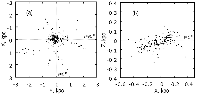
Рис. 1: (a) Distribution of stars on the Galactic XY plane; the circle marks the neighborhood the distribution of stars from which is shown on the XZ plane on panel (b).

1.2 Line-of-Sight Velocities

In addition to the main source, the Sb9 bibliographic database on the orbits of spectroscopic binaries (Pourbaix et al. 2004), we used the most recent orbit determinations for a number of stars, for example, the results from Rauw et al. (2012), Williams et al. (2013), and Mahy et al. (2013).

Note that the SIMBAD search database sometimes contains significant inaccuracies with regard to the line-of-sight velocities for spectroscopic binaries. For example, $V_{r}=-101\pm 20$ km s^-1 for the star V1034 Sco (O9.5+B1.5) from the list by Torres et al. (2010), while, according to Sana et al. (2005), $V_{\gamma}=-16.0\pm 1.5$ km s^-1.

After checking against the Sb9 database, we took the line-of-sight velocities of all spectroscopic binaries from the latest publications. Therefore, there are significant deviations from the data of the Gontcharov (2006) or CRVAD-2 (Kharchenko et al. 2007) catalogs for many of them.

As was pointed out in Moffat et al. (1998), determining realistic values of the systemic line-of-sight velocities is very difficult for O stars and virtually impossible for Wolf–Rayet stars. Therefore, we tried to include as few data on Wolf–Rayet stars as possible in our sample.

1.3 Proper Motions

We took most of the stellar proper motions from the Hipparcos catalogue (van Leeuwen 2007). For 17 systems that do not enter into the Hipparcos list, we used data from the UCAC4 (Zacharias 2012), Tycho-2 (Hog et al. 2000), CRVAD-2 (Kharchenko et al. 2007), and PPMXL (Roeser et al. 2010) catalogues.

Thus, O stars, for example, almost all spectroscopic binary O stars from the GOS2 catalogue (Maiz-Apellániz et al. 2004) are reflected in our sample to a maximum degree. Only the stars with the ‘‘runaway’’ status were rejected.

2 KINEMATIC ANALYSIS

2.1 Galactic Rotation Model

The method of determining the kinematic parameters applied here consists in minimizing a quadratic functional F:

$$\min\leavevmode\nobreak\ F=\sum_{j=1}^{N}w_{r}^{j}(V_{r}^{j}-\hat{V}_{r}^{j})^{2}+\sum_{j=1}^{N}w_{l}^{j}(V_{l}^{j}-\hat{V}_{l}^{j})^{2}+\sum_{j=1}^{N}w_{b}^{j}(V_{b}^{j}-\hat{V}_{b}^{j})^{2}$$ (1)

provided the fulfilment of the following constraints derived from Bottlinger’s formulas with an expansion of the angular velocity of Galactic rotation $\Omega$ into a series to terms of the second order of smallness with respect to $r/R_{0}$ and with allowance made for the influence of the spiral density wave:

$$\begin{array}[]{lll}V_{r}&=&-u_{\odot}\cos b\cos l-v_{\odot}\cos b\sin l-w_{\odot}\sin b\\ &+&R_{0}(R-R_{0})\sin l\cos b\Omega^{\prime}_{0}\\ &+&0.5R_{0}(R-R_{0})^{2}\sin l\cos b\Omega^{\prime\prime}_{0}\\ &+&\Delta V_{rot}\sin(l+\theta)\cos b,\\ &-&V_{R}\cos(l+\theta)\cos b,\end{array}$$ (2)

$$\begin{array}[]{lll}V_{l}&=&u_{\odot}\sin l-v_{\odot}\cos l\\ &+&(R-R_{0})(R_{0}\cos l-r\cos b)\Omega^{\prime}_{0}\\ &+&(R-R_{0})^{2}(R_{0}\cos l-r\cos b)0.5\Omega^{\prime\prime}_{0}-r\Omega_{0}\cos b\\ &+&\Delta V_{rot}\cos(l+\theta)+V_{R}\sin(l+\theta),\end{array}$$ (3)

$$\begin{array}[]{lll}V_{b}&=&u_{\odot}\cos l\sin b+v_{\odot}\sin l\sin b-w_{\odot}\cos b\\ &-&R_{0}(R-R_{0})\sin l\sin b\Omega^{\prime}_{0}\\ &-&0.5R_{0}(R-R_{0})^{2}\sin l\sin b\Omega^{\prime\prime}_{0}\\ &-&\Delta V_{rot}\sin(l+\theta)\sin b,\\ &+&V_{R}\cos(l+\theta)\sin b,\end{array}$$ (4)

where the following notation is used: $N$ is the number of stars used; $j$ is the current star number; $V_{r}$ is the line-of-sight velocity, $V_{l}=4.74r\mu_{l}\cos b$ and $V_{b}=4.74r\mu_{b}$ are the proper motion velocity components in the $l$ and $b$ directions, respectively, with the coefficient 4.74 being the quotient of the number of kilometers in an astronomical unit and the number of seconds in a tropical year; $\hat{V}_{r}^{j},\hat{V}_{l}^{j},\hat{V}_{b}^{j}$ are the measured components of the velocity field (data); $w_{r}^{j},w_{l}^{j},w_{b}^{j}$ are the weight factors; the star’s proper motion components $\mu_{l}\cos b$ and $\mu_{b}$ are in mas yr^-1 and the line-of-sight velocity $V_{r}$ is in km s^-1; $u_{\odot},v_{\odot},w_{\odot}$ are the stellar group velocity components relative to the Sun taken with the opposite sign (the velocity $u$ is directed toward the Galactic center, $v$ is in the direction of Galactic rotation, $w$ is directed to the north Galactic pole); $R_{0}$ is the Galactocentric distance of the Sun; $R$ is the Galactocentric distance of the star; $\Omega_{0}$ is the angular velocity of rotation at the distance $R_{0}$; the parameters $\Omega^{\prime}_{0}$ and $\Omega^{\prime\prime}_{0}$ are the first and second derivatives of the angular velocity, respectively; the distance $R$ is calculated from the formula

$$\begin{array}[]{lll}R^{2}=r^{2}\cos^{2}b-2R_{0}r\cos b\cos l+R^{2}_{0}.\end{array}$$ (5)

To take into account the influence of the spiral density wave, we used the simplest kinematic model based on the linear density wave theory by Lin et al. (1969), in which the potential perturbation is in the form of a traveling wave. Then,

$$\begin{array}[]{lll}V_{R}=&f_{R}\cos\chi,\end{array}$$ (6)

$$\begin{array}[]{rll}\Delta V_{rot}=&f_{\theta}\sin\chi,\end{array}$$ (7)

where $f_{R}$ and $f_{\theta}$ are the amplitudes of the radial (directed toward the Galactic center in the arm) and azimuthal (directed along the Galactic rotation) velocity perturbations; $i$ is the spiral pitch angle ($i<0$ for winding spirals); $m$ is the number of arms, we take $m=2$ in this paper; $\theta$ is the star’s position angle (measured in the direction of Galactic rotation): $\tan\theta=y/(R_{0}-x)$, where $x$ and $y$ are the Galactic heliocentric rectangular coordinates of the object; the wave phase $\chi$ is

$$\chi=m[\cot(i)\ln(R/R_{0})-\theta]+\chi_{\odot},$$ (8)

where $\chi_{\odot}$ is the Sun’s radial phase in the spiral density wave; we measure this angle from the center of the Carina–Sagittarius spiral arm ($R\approx 7$ kpc). The parameter $\lambda$, the distance (along the Galactocentric radial direction) between adjacent segments of the spiral arms in the solar neighborhood (the wavelength of the spiral density wave), is calculated from the relation

$$\frac{2\pi R_{0}}{\lambda}=m\cot(i).$$ (9)

The weight factors in functional (1) are assigned according to the following expressions (for simplification, we omitted the index $i$)

$$w_{r}=S_{0}/\sqrt{S_{0}^{2}+\sigma^{2}_{V_{r}}},\quad w_{l}=\beta^{2}S_{0}/\sqrt{S_{0}^{2}+\sigma^{2}_{V_{l}}},\quad w_{b}=\gamma^{2}S_{0}/\sqrt{S_{0}^{2}+\sigma^{2}_{V_{b}}},$$ (10)

where $S_{0}$ denotes the dispersion averaged over all observations, which has the meaning of a ‘‘cosmic’’ dispersion taken to be 8 km s^-1; $\beta=\sigma_{V_{r}}/\sigma_{V_{l}}$ and $\gamma=\sigma_{V_{r}}/\sigma_{V_{b}}$ are the scale factors that we determined using data on open star clusters (Bobylev et al. 2007), $\beta=1$ and $\gamma=2$. The errors of the velocities $V_{l}$ and $V_{b}$ are calculated from the formula

$$\sigma_{(V_{l},V_{b})}=4.74r\sqrt{\mu^{2}_{l,b}\Biggl{(}{\sigma_{r}\over r}\Biggr{)}^{2}+\sigma^{2}_{\mu_{l,b}}}.$$ (11)

The optimization problem (1)–(8) is solved for the unknown parameters $u_{\odot},$ $v_{\odot},$ $w_{\odot},$ $\Omega_{0}$, $\Omega^{\prime}_{0},$ $\Omega^{\prime\prime}_{0},$ $f_{R},$ $f_{\theta},$ $i$ and $\chi_{\odot}$ by the coordinate-wise descent method.

We estimated the errors of the sought-for parameters through Monte Carlo simulations. The errors were estimated by performing 1000 cycles of computations. For this number of cycles, the mean values of the solutions essentially coincide with the solutions obtained from the input data without any addition of measurement errors. Measurements errors were added to such input data as the line-of-sight velocities, proper motions, and distances.

We take $R_{0}=8.0\pm 0.4$ kpc according to the result of analyzing the most recent determinations of this quantity in the review by Foster and Cooper (2010).

2.2 Periodogram Analysis of Residual Velocities

Relation (8) for the phase can be expressed in terms of the perturbation wavelength $\lambda$, which is equal to the distance between the adjacent spiral arms along the Galactic radius vector. Using relation (9) between the pitch angle $i$ and wavelength $\lambda$ (9), we will obtain an expression for the phase as a function of the star’s Galactocentric distance $R$ and position angle $\theta$:

$$\chi=\frac{2\pi R_{0}}{\lambda}\ln(R/R_{0})-m\theta+\chi_{\odot}.$$ (12)

The goal of our spectral analysis of the series of measured residual velocities $V_{R_{n}}$ and $\Delta V_{\theta_{n}},n=1,\dots,N$, where $N$ is the number of objects, is to extract the periodicity in accordance with model (6), (7), describing a spiral density wave with parameters $f_{R},f_{\theta},\lambda$ and $\chi_{\odot}$. If the wavelength $\lambda$ is known, then the pitch angle $i$ is easy to determine from Eq. (9) by specifying the number of arms $m.$ Here, we adopt a two-armed model, i.e., $m=2.$

Let us form the initial series of velocity perturbations (6), (7) for Galactic objects in the most general, complex form:

$$V_{n}=V_{R_{n}}+j\Delta V_{\theta_{n}},$$ (13)

where $j=\sqrt{-}1$, $n$ is the object number ($n=1,...,N).$ A periodogram analysis consists in calculating the amplitude of the spectrum squared (power spectrum) obtained by expanding series (13) in terms of orthogonal harmonic functions $\exp[-j(2\pi R_{0}/\lambda_{k})\ln(R_{n}/R_{0})+jm\theta_{n}]$ in accordance with Eq. (12) for the phase of the spiral density wave to extract significant peaks in it.

Let us first calculate the complex spectrum of our series:

$$\begin{array}[]{lll}\bar{V}_{\lambda_{k}}=\bar{V}_{\lambda_{k}}^{Re}+j\bar{V}_{\lambda_{k}}^{Im}=\\ \frac{1}{N}\sum_{n=1}^{N}(V_{R_{n}}+j\Delta V_{\theta_{n}})\exp[-j\frac{\displaystyle 2\pi R_{0}}{\displaystyle\lambda_{k}}\ln(R_{n}/R_{0})+jm\theta_{n}],\end{array}$$ (14)

where the superscripts $Re$ and $Im$ denote the real and imaginary parts of the spectrum.

Let us reduce the problem of calculating spectrum (14) to the standard Fourier transform. Obviously, transformation (14) can be represented as

$$\begin{array}[]{lll}\bar{V}_{\lambda_{k}}=\frac{1}{N}\sum_{n=1}^{N}(V_{R_{n}}+j\Delta V_{\theta_{n}})\exp(j{\rm m}\theta_{n})\exp[-j\frac{\displaystyle 2\pi R_{0}}{\displaystyle\lambda_{k}}\ln(R_{n}/R_{0})]=\\ =\frac{1}{N}\sum_{n=1}^{N}V_{n}^{{}^{\prime}}\exp[-j\frac{\displaystyle 2\pi R_{0}}{\displaystyle\lambda_{k}}\ln(R_{n}/R_{0})],\end{array}$$ (15)

where

$$\begin{array}[]{lll}V_{n}^{{}^{\prime}}=V_{n}^{Re}+jV_{n}^{Im}=\\ =[V_{R_{n}}\cos(m\theta_{n})-\Delta V_{\theta_{n}}\sin(m\theta_{n})]+j[V_{R_{n}}\sin(m\theta_{n})+\Delta V_{\theta_{n}}\cos(m\theta_{n})].\end{array}$$ (16)

Finally, making the change of variables

$$R_{n}^{{}^{\prime}}=R_{0}\ln(R_{n}/R_{0}),$$ (17)

we will obtain the standard Fourier transform of the sequence $V_{n}^{{}^{\prime}}$, precalculated from Eq. (16) and defined in the space of coordinates $R_{n}^{{}^{\prime}}$ (17):

$$\bar{V}_{\lambda_{k}}=\frac{1}{N}\sum_{n=1}^{N}V_{n}^{{}^{\prime}}\exp[-j\frac{2\pi R_{n}^{{}^{\prime}}}{\lambda_{k}}].$$ (18)

The periodogram $|\bar{V}_{\lambda_{k}}|^{2}$ from which the statistically significant peak whose coordinate determines the sought-for wavelength $\lambda$ and, accordingly, the pitch angle of the spiral density wave $i$ (see (9)) is extracted is to be analyzed further. Obviously, our spectral analysis of the complex sequence (13) composed of the radial and tangential residual velocities does not allow the radial and tangential perturbation amplitudes to be separated. A separate analysis of the radial, $\{V_{R_{n}}\}$, and tangential residual, $\{\Delta V_{\theta_{n}}\}$, velocities, for example, as was shown in Bajkova and Bobylev (2012), is required to estimate the perturbation amplitudes $f_{R}$ and $f_{\theta}$. The input data $V_{n}^{{}^{\prime}}(R^{{}^{\prime}})(n=1,\dots,N)$ should be specified on a discrete mesh $l=1,\dots,K=2^{\alpha}$, $\alpha$ is an integer $>0$, $N\leq K$; $\Delta_{R}$, for a numerical realization of the Fourier transform (18), for example, using fast algorithms. The coordinates of the data are defined as numbers rounded off to an integer as follows: $l_{n}\approx[(R_{n}^{{}^{\prime}}+|\min\{R_{k}^{{}^{\prime}}\}|_{k=1,...,N})/\Delta_{R}+1],n=1,...,N$. is the discretization interval. The specified sequence of data is assumed to be periodic, with its period being $D=K\times\Delta_{R}$. The perturbation amplitudes are assumed to be zero at the points $l$ where there are no measurements.

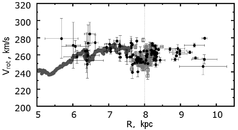
Рис. 2: Rotation velocities of stars around the Galactic center $V_{rot}$ versus Galactocentric distance $R$: the thick line indicates the velocities of neutral hydrogen (McClure-Griffiths and Dickey 2007); the black circles with bars are massive spectroscopic binaries; the grays squares are massive Hipparcos B stars whose parallaxes were determined with errors of no more than 10%.

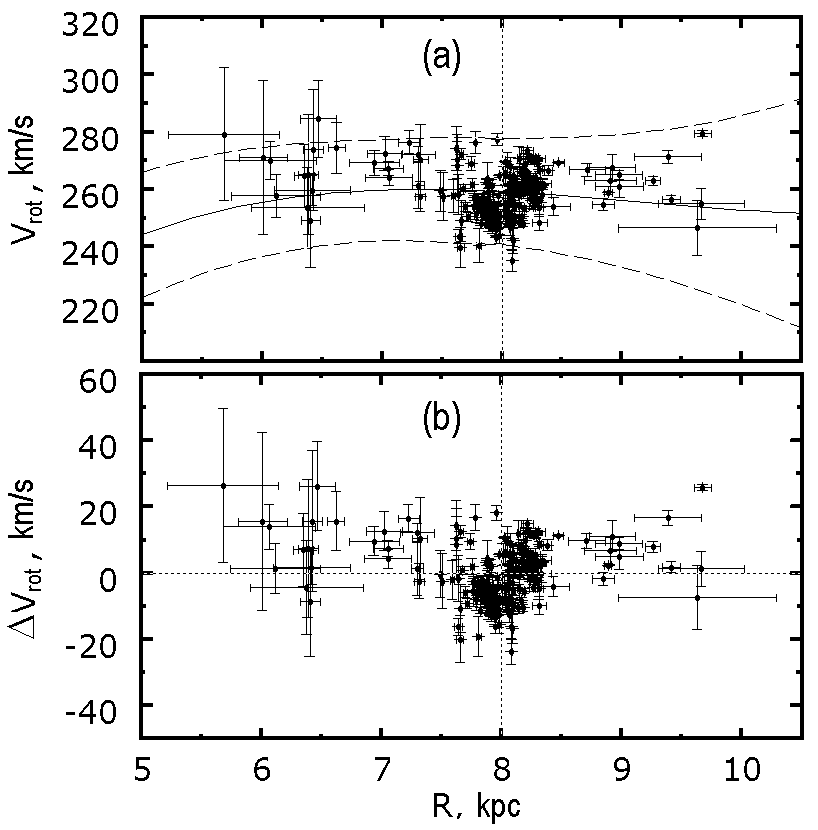
Рис. 3: (a) Galactic rotation curve; the vertical dotted line marks the position of the solar circle; the dashed lines indicate the boundaries of the 1у confidence intervals. (b) The residual velocities obtained relative to the rotation curve shown above.

3 RESULTS AND DISCUSSION

3.1 Galactic Rotation Parameters

First, we obtained the solution based on a sample of 97 spectroscopic binaries (the rejected systems are listed in Section 3.5) using only two equations, (2) and (3). This is because the contribution from Eq. (4) to the general solution is negligible when using distant stars. The velocity $w_{\odot}$ was assumed to be known (because it is determined very poorly from distant stars) and was taken to be $w_{\odot}=7$ km s^-1. Such an approach was used, for example, by Mishurov and Zenina (1999). The results turned out to be the following: $(u_{\odot},v_{\odot})=(3.3,8.8)\pm(0.9,1.3)$ km s^-1 and

$$\begin{array}[]{lll}\Omega_{0}=32.5\pm 1.1\leavevmode\nobreak\ \hbox{km s${}^{-1}$ kpc${}^{-1}$},\\ \Omega^{{}^{\prime}}_{0}=-4.41\pm 0.19\leavevmode\nobreak\ \hbox{km s${}^{-1}$ kpc${}^{-2}$},\\ \Omega^{{}^{\prime\prime}}_{0}=0.97\pm 0.37\leavevmode\nobreak\ \hbox{km s${}^{-1}$ kpc${}^{-3}$},\\ f_{R}=-11.5\pm 1.9\leavevmode\nobreak\ \hbox{km s${}^{-1}$},\\ f_{\theta}=5.5\pm 1.6\leavevmode\nobreak\ \hbox{km s${}^{-1}$},\\ i=-6.4^{\circ}\pm 0.6^{\circ},\\ \chi_{\odot}=-117^{\circ}\pm 6^{\circ},\end{array}$$ (19)

The error per unit weight is $\sigma_{0}=8.5$ km s^-1. Based on the derived pitch angle i and Eq. (9), we find $\lambda=2.8\pm 0.3$ kpc.

Since the solution using nearby Hipparcos B stars is of interest, we obtained the solution using the entire sample (220 stars). All three equations (2)–(4) were used in this approach; the velocity $w_{\odot}$ was not fixed. The results turned out to be the following: $(u_{\odot},v_{\odot},w_{\odot})=(3.4,8.9,7.8)\pm(0.8,1.1,0.2)$ km s^-1 and

$$\begin{array}[]{lll}\Omega_{0}=32.4\pm 1.1\leavevmode\nobreak\ \hbox{km s${}^{-1}$ kpc${}^{-1}$},\\ \Omega^{{}^{\prime}}_{0}=-4.33\pm 0.19\leavevmode\nobreak\ \hbox{km s${}^{-1}$ kpc${}^{-2}$},\\ \Omega^{{}^{\prime\prime}}_{0}=0.77\pm 0.42\leavevmode\nobreak\ \hbox{km s${}^{-1}$ kpc${}^{-3}$},\\ f_{R}=-10.8\pm 1.2\leavevmode\nobreak\ \hbox{km s${}^{-1}$},\\ f_{\theta}=7.9\pm 1.3\leavevmode\nobreak\ \hbox{km s${}^{-1}$},\\ i=-6.0^{\circ}\pm 0.4^{\circ},\\ \chi_{\odot}=-120^{\circ}\pm 4^{\circ},\end{array}$$ (20)

The error per unit weight is $\sigma_{0}=6.5$ km s^-1, $\lambda=2.6\pm 0.2$ kpc and the linear rotation velocity of the Galaxy is $V_{0}=|R_{0}\Omega_{0}|=259\pm 16$ km s^-1 (at $R_{0}=8$ kpc).

From our comparison of results (19) and (20) we see that the most distant stars have a decisive effect when finding the Galactic rotation parameters. Using a large number of nearby stars with highly accurate distances reduces only slightly the errors of the parameters being determined. On the other hand, in solution (20) the velocity $w_{\odot}$ is determined well and the tangential perturbation amplitude $f_{\theta}$ increases.

The derived parameters of the Galactic rotation curve are in good agreement with the results of analyzing young Galactic disk objects rotating most rapidly around the center, such as OB associations, $\Omega_{0}=-31\pm 1$ km s^-1 kpc^-1 (Melńik et al. 2001; Melńik and Dambis 2009), blue supergiants, $\Omega_{0}=-29.6\pm 1.6$ km s^-1 kpc^-1 and $\Omega^{\prime}_{0}=4.76\pm 0.32$ km s^-1 kpc^-2 (Zabolotskikh et al. 2002), or OB3 stars, $\Omega_{0}=-31.5\pm 0.9$ km s^-1 kpc^-1, $\Omega^{{}^{\prime}}_{0}=+4.49\pm 0.12$ km s^-1 kpc^-2, and $\Omega^{{}^{\prime\prime}}_{0}=-1.05\pm 0.38$ km s^-1 kpc^-3 (Bobylev and Bajkova 2011).

As can be seen from Fig. 2, the patterns of change in the rotation velocities of stars and hydrogen clouds are similar at $R>7$ kpc, i.e., the phases of the velocity perturbations produced by the spiral density wave are similar. The significant velocity dispersion of OB stars at distances $R\approx 6$ kpc is caused by the proper motion errors.

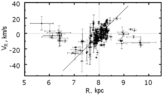
Рис. 4: Galactocentric radial velocities of the sample stars $V_{R}$ versus distance $R$; the vertical line marks the position of the solar circle.

Figure 3a presents the rotation velocities of the stars from our entire sample and the Galactic rotation curve constructed in accordance with solution (20). The confidence intervals were calculated by taking into account the uncertainty in $R_{0}.$ Figure 3b presents the residual velocities $\Delta V_{rot}$ calculated using the derived Galactic rotation curve.

In Fig. 4, the Galactocentric radial velocities ($V_{R}$) of the sample stars are plotted against distance $R$. The periodicity related to the influence of the spiral density wave is clearly seen. We plotted the line whose slope to the horizontal axis is equal to the radial velocity gradient $dV_{R}/dR\approx 40$ km s^-1 kpc^-1 near $R=R_{0}$ (this gradient will be considered in more detail in Section 3.3).

To construct the curves in Figs. 3 and 4, we used the stellar velocities calculated with the following parameters of the local standard of rest: $(U_{\odot},V_{\odot},W_{\odot})_{LSR}=(11.1,12.2,7.3)$ km s^-1 (Schönrich et al. 2010). It can be clearly seen from Fig. 4 that all distant stars are shifted downward by $\approx$6 km s^-1 ($\Delta U_{\odot}$). The point is that so significant an effect was detected neither in Bobylev and Bajkova (2011), where the kinematics of OB3 stars was considered, nor in our papers aimed at analyzing Galactic masers (Bobylev and Bajkova 2010; Bajkova and Bobylev 2012).

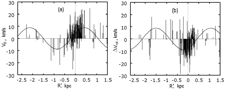
Рис. 5: (a) Galactocentric radial velocities $V_{R}$ for 220 stars versus distance $R^{\prime}$; (b) residual rotation velocities $\Delta V_{rot}$; the velocities are given relative to the group velocity found.

In Fig. 5, the radial, $V_{R},$ and residual tangential, $\Delta V_{rot}$, velocities for the stars of the entire sample are plotted against distance $R^{\prime}$, with these velocities being given relative to the group velocity $(u_{\odot},v_{\odot},w_{\odot})$ found in solution (20). The power spectrum corresponding to this approach is shown in Fig. 6.

Our comparison of solutions (19) and (20) and the results of our spectral analysis of the residual velocities presented in Figs. 5 and 6 lead us to conclude that the derived spiral density wave parameters agree well between themselves. Thus, the wavelength is $\lambda=2.6$ kpc and the phase is $\chi_{\odot}=-120^{\circ}$. However, these values still differ from $\lambda=2.3\pm 0.2$ kpc and $\chi_{\odot}=-91^{\circ}\pm 4^{\circ}$ that were found in our previous paper from OB3 stars using an independent distance scale (Bobylev and Bajkova 2011), which will be discussed in Section 3.4. As can be seen from Fig. 6, the spectral peak is well extracted, although the spectrum has a large low-frequency component.

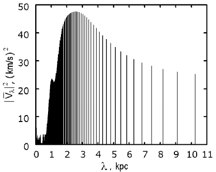
Рис. 6: Power spectrum of the velocities for the entire sample of stars.

3.2 Residual Velocities

The stellar velocities corrected both for the Galactic differential rotation and for the influence of the spiral density wave are presented in Fig. 7 for distant stars ($r>0.6$ kpc) and in Fig. 8 for nearby stars ($r\leq 0.6$ kpc). The diagonal lines in Figs. 7a and 8a indicate the orientation of the velocity ellipsoid on the UV plane typical of the Gould Belt stars (Bobylev 2006). As can be seen from Figs. 7d and 8d, applying a correction for the influence of the spiral structure removes the elongation and makes the distribution of stars nearly circular.

For example, for nearby stars before applying any corrections for the influence of the density wave (this case corresponds to Figs. 8a–8c), the means are $({\overline{U}},{\overline{V}},{\overline{W}})=(-10.0,-14.7,-7.2)$ km s^-1 (as we see, the magnitudes of these velocities differ little from the solar motion parameters derived by Schönrich et al. (2010). In this case, the principal axes of the velocity ellipsoid are $(\sigma_{U},\sigma_{V},\sigma_{W})=(7.3,5.7,3.8)\pm(0.5,0.6,0.4)$ km s^-1; the orientation of the first axis ($l_{1}=308\pm 7^{\circ},b_{1}=1\pm 1^{\circ}$) is shown in Fig. 8a. Once the corrections for the influence of the density wave have been applied (this case corresponds to Figs. 8d.8f), the coordinates of the distribution center and the velocity dispersions are $({\overline{U}},{\overline{V}},{\overline{W}})=(-4.5,-8.6,-7.2)$ km s^-1 and $(\sigma_{U},\sigma_{V},\sigma_{W})=(6.1,5.8,3.7)\pm(0.6,0.5,0.4)$ km s^-1, and the orientation of the velocity ellipsoid essentially coincides with the directions of the $X,Y,Z$ coordinate axes.

3.3 Kinematic Peculiarities of the Gould Belt

When studying stars belonging to the Gould Belt, various authors have long noticed such a kinematic effect as the expansion of this entire star system with an expansion parameter $k\approx 25$ km s^-1 kpc^-1 (Bobylev 2006). A similar effect with an expansion parameter $k\approx 46$ km s^-1 kpc^-1 is also detected in one of the components of the Gould Belt, the vast Scorpius–Centaurus OB association (Bobylev and Bajkova 2007). Torres et al. (2008) showed that the centers of all small associations ($\beta$ Pic, Tuc-Hor, TW Hya, and others) in the neighborhood of Scorpius–Centaurus have an expansion parameter of 50 km s^-1 kpc^-1.

The radial velocity gradient $dVR/dR\approx 40$ km s^-1 kpc^-1 indicated in Fig. 4 is very close to the above local expansion parameters. However, remaining within the theory of the influence of the spiral density wave, we must conclude that the influence of the Galactic density wave should first be taken into account to properly determine the intrinsic expansion parameters of the Scorpius–Centaurus OB association and the entire Gould Belt.

For example, the elongation of the velocity ellipsoid along the diagonal in Fig. 8a is the most important indicator for the presence of intrinsic expansion. contraction effects in the system. However, as can be seen from Fig. 8d, such an elongation is removed almost completely once the parameters of the spiral density wave have been taken into account. This fact leaves fewer chances for the implementation of a simple expansion model of the Gould Belt as a whole. Studying this question is not the main task of this paper; it will be considered in another paper.

Studying the influence of a large number of nearby Gould Belt stars on our solutions (19) and (20) is also of interest. In particular, the influence of the intrinsic kinematics of the Gould Belt can be responsible for the discrepancy between the phase angle $\chi_{\odot}=-120^{\circ}\pm 4^{\circ}$ (solution (20)) and $\chi_{\odot}=-91^{\circ}\pm 4^{\circ}$ found from OB3 stars (at $r>0.8$ kpc) using the ‘‘calcium’’ distance scale (Bobylev and Bajkova 2011). To test this assumption, we obtained the solution based on a sample free from Gould Belt stars.

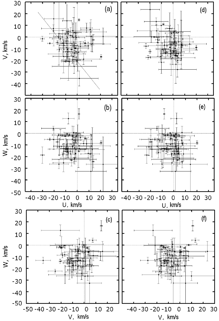
Рис. 7: Residual velocities $U,V,W$ of 58 distant stars relative to the Sun: (a), (b), (c) corrected for the Galactic differential rotation; (d), (e), (f) additionally corrected for the influence of the Galactic spiral density wave.

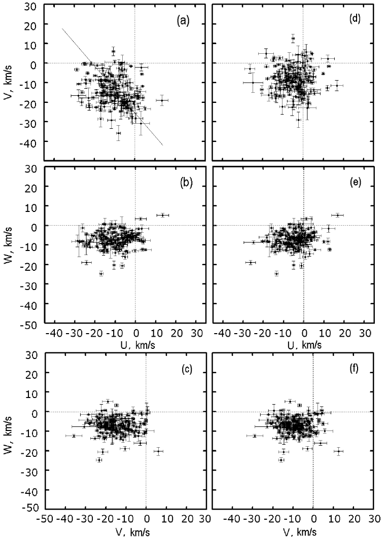
Рис. 8: Residual velocities $U,V,W$ of 162 nearby stars relative to the Sun: (a), (b), (c) corrected for the Galactic differential rotation; (d), (e), (f) additionally corrected for the influence of the Galactic spiral density wave.

3.4 Galactic Kinematics from Distant Stars

Based on the approach described when obtaining solution (19) and using 58 distant stars located outside the circle with a radius of 0.6 kpc containing the Gould Belt stars (Fig. 1), we found the following sought-for parameters: $(u_{\odot},v_{\odot})=(2.2,8.4)\pm(0.9,1.1)$ km s^-1 and

$$\begin{array}[]{lll}\Omega_{0}=31.9\pm 1.1\leavevmode\nobreak\ \hbox{km s${}^{-1}$ kpc${}^{-1}$},\\ \Omega^{{}^{\prime}}_{0}=-4.30\pm 0.16\leavevmode\nobreak\ \hbox{km s${}^{-1}$ kpc${}^{-2}$},\\ \Omega^{{}^{\prime\prime}}_{0}=1.05\pm 0.35\leavevmode\nobreak\ \hbox{km s${}^{-1}$ kpc${}^{-3}$},\\ f_{R}=-10.8\pm 1.2\leavevmode\nobreak\ \hbox{km s${}^{-1}$},\\ f_{\theta}=2.9\pm 2.1\leavevmode\nobreak\ \hbox{km s${}^{-1}$},\\ i=-7.3^{\circ}\pm 0.5^{\circ},\\ \chi_{\odot}=-104^{\circ}\pm 6^{\circ}.\end{array}$$ (21)

The error per unit weight is $\sigma_{0}=9.9$ km s^-1, the wavelength is $\lambda=3.2\pm 0.3$ kpc, and $V_{0}=255\pm 16$ km s^-1. Figure 9 presents the results of our spectral analysis of the radial velocities (our analysis of the residual tangential velocities did not give a statistically significant perturbation amplitude). The wavelength of the radial velocity perturbations is $\lambda=2.7$ kpc, which is slightly lower than that obtained by solving the kinematic equations. The significance of the peak is very high. Owing to the removal of nearby stars from the spectrum, the low-frequency part decreased compared to the spectrum shown in Fig. 6.

The velocity $V_{0}$ is of great importance for constructing an appropriate Galactic rotation model and a model of the Galactic potential. For example, the Galactic rotation curve constructed by Sofue et al. (2009) with the adopted $R_{0}=8$ kpc and $V_{0}=200$ km s^-1 close to the parameters recommended by the IAU (1985) is well known. However, a kinematic analysis of OB stars (Zabolotskikh et al. 2002) or masers (Reid et al. 2009; McMillan and Binney 2010; Bajkova and Bobylev 2012) shows that $V_{0}$ for the youngest disk objects is slightly larger, being 240–260 km s^-1. Note the paper by Irrgang et al. (2013), where three models of the Galactic potential constructed using data on hydrogen clouds and masers were proposed, with $V_{0}$ having been found to be close to 240 km s^-1 (at $R_{0}\approx 8.3$ kpc).

There are two parameters in solution (21), $\chi_{\odot}$ and $f_{\theta}$, whose values differ significantly from those obtained in solutions (19) and (20). Now, the amplitude ratio and the Sun’s phase are in agreement with the results of analyzing blue supergiants, $f_{R}=-6.6\pm 2.5$ km s^-1, $f_{\theta}=0.4\pm 2.3$ km s^-1, and $\chi_{\odot}=-97^{\circ}\pm 18^{\circ}$ (Zabolotskikh et al. 2002), and in agreement with $f_{R}=-13\pm 1$ km s^-1, $f_{\theta}=0\pm 1$ km s^-1, and $\chi_{\odot}=-91^{\circ}\pm 4^{\circ}$ found from a sample of 102 distant OB3 stars (Bobylev and Bajkova 2011).

The following conclusions can be reached: (1) Gould Belt stars affect significantly the results of our analysis of the tangential velocities—it is these stars that make a major contribution to such a large $f_{\theta}=7.9\pm 1.3$ km s^-1 in solution (20); (2) including Gould Belt stars in the sample leads to a noticeable shift of the Sun’s phase in the density wave, $\chi_{\odot}=-120^{\circ}\pm 4^{\circ}$, compared to $\chi_{\odot}=-104^{\circ}\pm 6^{\circ}$ found from distant stars. Note that there was no such problem when we determined the spiral density wave parameters from Cepheids (Bobylev and Bajkova 2012), because Cepheids are not associated kinematically with the Gould Belt.

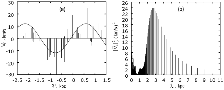
Рис. 9: (a) Galactocentric radial velocities $V_{R}$ of 58 distant stars versus distance $R^{\prime}$ and (b) their power spectrum.

3.5 Candidates for Runaway Stars

The spiral density wave can produce a noticeable velocity perturbation for some of the stars reaching 10–15 km s^-1, depending on their positions in the spiral wave. Therefore, when determining the status of a star as a runaway, we consider the residual velocities calculated by taking into account the density wave parameters found. We obtained the following results.

(1) According to the estimate by Torres et al. (2010), the eclipsing spectroscopic binary DW Car (B1V+B1V; 11M_⊙+11M_⊙) is located at a heliocentric distance of $2840\pm 150$ pc. It does not enter into the Hipparcos list of stars. According to the UCAC4 data, its proper motion components are $\mu_{\alpha}\cos\delta=-12.8\pm 1.6$ mas yr^-1 and $\mu_{\delta}=-1.1\pm 1.1$ mas yr^-1. Similar values were also obtained in the TRC catalogue (Hog et al. 1998). The line-of-sight velocity is $V_{\gamma}=-7.3\pm 3.7$ km s^-1 (Southworth and Clausen 2007). We found it to have a huge peculiar velocity at these parameters, $|V_{pec}|=113\pm 28$ km s^-1.

(2) The SB2 system DH Cep (O5.5V+O6.5V) has a significant residual velocity, $|V_{pec}|=44\pm 15$ km s^-1. We used a distance estimate of $2767\pm 450$ pc for it (Hilditch et al. 1996). However, it is not marked as a runaway in the GOS2 catalogue (Maiz-Apellańiz et al. 2004).

(3) The distant SB systemHD1383 (B0.5I+B0.5I) located at a distance of $2860\pm 570$ pc (Gudennavar et al. 2012) has $|V_{pec}|=40\pm 14$ km s^-1.

(4) HD 150136 (HR 6187; O3V+O5.5+O6.5V) located at a distance of $1320\pm 120$ pc recently classified by Mahy et al. (2012) as a spectroscopic triple system has $|V_{pec}|=36\pm 10$ km s^-1.

(5) The binary system V 1034 Sco (O9V+B1.5V; 17M_⊙+9.6M_⊙) from the list by Torres et al. (2010), $r=1640\pm 89$ pc, does not enter into the Hipparcos list of stars. It does not have a large peculiar velocity ($|V_{pec}|=28\pm 17$ km s^-1), but it is always rejected according to the $3\sigma$ criterion. The proper motion components (UCAC4) for it are probably not quite reliable.

(6) Finally, the star HIP 99303 (V1624 Cyg, B2.5V), $r=318\pm 23$ pc, is rejected according to the $3\sigma$ criterion, although its peculiar velocity is small, $|V_{pec}|=28\pm 2$ km s^-1.

As can be seen from this list, two stars, DW Car and the SB2 system DH Cep, can be attributed with a high degree of reliability to runaway stars, because their peculiar velocities exceed 40 km s^-1. The star DW Car whose peculiar velocity exceeds 100 km s^-1 especially stands out.

We excluded the listed stars when solving Eqs. (2)–(4). However, as our analysis that is not presented here showed, the line-of-sight velocities of these stars are quite acceptable and can be used in Eqs. (2)–(4). They are not rejected according to the $3\sigma$ criterion and do not spoil the solutions.

4 DESCRIPTION OF THE DATABASE

The data format is described in Table 3. Note that two values are given for the line-of-sight velocity error, $\varepsilon_{V_{r}}$ and $\sigma_{V_{r}}$. The quantity $\varepsilon_{V_{r}}$ is the formal random error in the systemic velocity $V_{\gamma}$ when interpreting the line-of-sight velocity curves; its value can be very low, $<0.05$ km s^-1, for a number of stars (in such cases, they were rounded off to 0.1 km s^-1). The quantity $\sigma_{V_{r}}$ characterizes the quality of the observed line-of-sight velocities as a whole—we used this quantity to assign the individual weights of the stars when solving the system of equations (2)–(4). As $\sigma_{V_{r}}$ we took either the dispersion of the residuals that the authors usually specify (r.m.s) and, in the case of its absence, the errors in the velocity amplitude for the first component (K1) of a spectroscopic binary system.

The peculiar space velocities of the stars were calculated by taking into account the Galactic differential rotation effects and the influence of the spiral density wave with the parameters found in solution (20). Information about the bibliography is given in Table 1.

Таблица 3: Format of the database

Alternative star name	A12
HD/CD/BD number	A12
Hipparcos number	A10
Right ascension in degrees	F11.6
Declination in degrees	F11.6
Heliocentric distance in pc	F6.1
Proper motion in right ascension in mas yr-1	F6.2
Proper motion in declination in mas yr-1	F6.2
Line-of-sight velocity in km s-1	F6.1
Heliocentric distance error in pc	F5.1
Error of proper motion in right ascension in mas yr-1	F4.2
Error of proper motion in declination in mas yr-1	F4.2
Line-of-sight velocity error in km s-1	F4.1
Line-of-sight velocity dispersion in km s-1	F4.1
Spectral type of first component	A10
Spectral type of second component	A8
Spectral type of third component	A5
Peculiar space velocity in km s-1	F5.1
Error of peculiar space velocity in km s-1	F4.1
Reference information	A14

CONCLUSIONS

Based on published sources, we created a kinematic database on massive ($>10M_{\odot}$) young Galactic star systems located within $\leq 3$ kpc of the Sun. For most of the stars within $\approx$600 pc of the Sun, the distance errors do not exceed 10%. We included all massive OB stars with known estimates of their orbital (dynamical) parallaxes; the errors in the dynamical distances for seven such systems are smaller than those in the trigonometric ones, with the errors for two of them being equal. Spectrophotometric distance estimates were used for more distant stars, but there are also calibration spectroscopic binary systems with very reliable distances among these objects. The main advantage of the proposed list of spectroscopic binary systems is that the latest information about the measured line-of-sight velocities and proper motions is reflected for them.

Based on the entire sample of 220 stars, we found the circular rotation velocity of the solar neighborhood around the Galactic center, $V_{0}=259\pm 16$ km s^-1 (at $R_{0}=8$ kpc), and the following spiral density wave parameters: the amplitudes of the radial and azimuthal velocity perturbations $f_{R}=-10.8\pm 1.2$ km s^-1 and $f_{\theta}=7.9\pm 1.3$ km s^-1, respectively; the pitch angle for a two-armed spiral pattern $i=-6.0^{\circ}\pm 0.4^{\circ}$ ($\lambda=2.6\pm 0.2$ kpc); and the radial phase of the Sun in the spiral density wave $\chi_{\odot}=-120^{\circ}\pm 4^{\circ}$. The residual velocity dispersion for the stars of the entire sample obtained by taking into account the Galactic differential rotation effects and the influence of the spiral density wave is $\sigma\approx 7$ km s^-1. This suggests that the stars are young and that their kinematic characteristics are close to those of hydrogen clouds, for which the residual velocity dispersion is 5.6 km s^-1.

Based on a sample of 58 distant ($r>0.6$ kpc) stars, we found the following parameters: $V_{0}=255\pm 16$ km s^-1, $f_{R}=-10.8\pm 1.2$ km s^-1, $f_{\theta}=2.9\pm 2.1$ km s^-1, $i=-7.3^{\circ}\pm 0.5^{\circ}$, and $\chi_{\odot}=-104^{\circ}\pm 6^{\circ}$. These are in good agreement with the results of analyzing other samples of OB stars by other authors. These parameters describe the properties of the Galactic grand-design spiral structure in the neighborhood under consideration.

Such peculiarities of the Gould Belt as the local expansion of the system, the velocity ellipsoid vertex deviation, and the significant additional rotation can be explained in terms of the density wave theory. All these effects decrease significantly once the influence of the spiral density wave on the velocities of these stars has been taken into account. Our study of the contribution from Gould Belt stars to the determination of the spiral density wave parameters showed that (1) these stars affect significantly the results of analyzing the tangential velocities—they make a major contribution to the large value of $f_{\theta}=7.9\pm 1.3\leavevmode\nobreak\ \hbox{\T2A\cyrk\T2A\cyrm/c}$ km s^-1; (2) including Gould Belt stars in the sample leads to a noticeable shift of the Sun’s phase in the density wave, $\Delta\chi_{\odot}=30^{\circ}$, compared to the value found from distant ($r>0.6$ kpc) stars. Among the list of calibration spectroscopic binary systems by Torres et al. (2010), the runaway star DW Car with a significant peculiar velocity, $|V_{pec}|=113\pm 28$ km s^-1, has probably been revealed for the first time. The SB2 system DH Cep also has an appreciable peculiar velocity, $|V_{pec}|=44\pm 15$ km s^-1.

REFERENCES

1. E. Anderson and S. Francis, Astron. Lett. 38, 331 (2012).

2. M. Ausseloos, C. Aerts, K. Lefever, et al., Astron. Astrophys. 455, 259 (2006).

3. V.C. Avedisova, Astron. Rep. 49, 435 (2005).

4. A.T. Bajkova and V.V. Bobylev, Astron. Lett. 38, 549 (2012).

5. H. Bakis, V. Bakis, O. Demircan, et al., Mon. Not. R. Astron. Soc. 385, 381 (2008).

6. V. Bakis, I. Bulut, S. Bilir, et al., Publ. Astron. Soc. Jpn. 62, 1291 (2010).

7. S.A. Bell, D. Kilkenny, and G.J. Malcolm, Mon. Not. R. Astron. Soc. 226, 879 (1987).

8. V.V. Bobylev, Astron. Lett. 32, 816 (2006).

9. V.V. Bobylev and A.T. Bajkova, Astron. Lett. 33, 571 (2007).

10. V.V. Bobylev and A.T. Bajkova, Mon. Not. R. Astron. Soc. 408, 1788 (2010).

11. V.V. Bobylev and A.T. Bajkova, Astron. Lett. 37, 526 (2011).

12. V.V. Bobylev and A.T. Bajkova, Astron. Lett. 38, 638 (2012).

13. V.V. Bobylev, A.T. Bajkova, and A. S. Stepanishchev, Astron. Lett. 34, 515 (2008).

14. R.L. Branham, Mon. Not. R. Astron. Soc. 370, 1393 (2006).

15. J.A. Caballero, Mon. Not. R. Astron. Soc. 383, 750 (2008).

16. D.P. Clemens, Astrophys. J. 295, 422 (1985).

17. A. Coleiro and S. Chaty, arXiv:1212.5460 (2012).

18. Z. Cvetković , I. Vince, and S. Ninković, New Astron. 15, 302 (2010).

19. J.A. Docobo and M. Andrade, Astrophys. J. 652, 681 (2006).

20. S.A. Dzib, L.F. Rodriguez, L.Loinard, et al., arXiv:1212.1498 (2012).

21. T. Foster and B. Cooper, astro-ph: 1009.3220 (2010).

22. G.A. Gontcharov, Astron. Lett. 32, 759 (2006).

23. S.B. Gudennavar, S.G. Bubbly, K. Preethi et al., Astrophys. J. Suppl. Ser. 199, 8 (2012).

24. T.J. Harries, R.W. Hilditch, and G. Hill, Mon. Not. R. Astron. Soc. 285, 277 (1997).

25. R.W. Hilditch, T.J. Harries, and S.A. Bell, Astron. Astrophys. 314, 165 (1996).

26. E. Hog, A. Kuzmin, U. Bastian, et al., Astron. Astrophys. 335, L65 (1998).

27. E. Hog, C. Fabricius, V.V. Makarov, et al., Astron. Astrophys. Lett. 355, L27 (2000).

28. M.M. Hohle, R. Neuhåuser, and B.F. Schutz, Astron. Nachr. 331, 349 (2010).

29. D.E. Holmgren, C.D. Scarfe, G. Hill, et al., Astron. Astrophys. 231, 89 (1990).

30. K. van der Hucht, New Astron. Rev. 45, 135 (2001).

31. A. Irrgang, B. Wilcox, E. Tucker, et al., Astron. Astrophys. 549, 137 (2013).

32. M. Kennedy, S.M. Dougherty, A. Fink, et al., Astrophys. J. 709, 632 (2010).

33. N.V. Kharchenko, A.E. Piskunov, S. Roeser, et al., Astron. Astrophys. 438, 1163 (2005).

34. N.V. Kharchenko, R.-D. Scholz, A.E. Piskunov, et al., Astron. Nachr. 328, 889 (2007).

35. M.K. Kim, T. Hirota, M. Honma, et al., Publ. Astron. Soc. Jpn. 60, 991 (2008)

36. S. Kraus, G. Weigelt, Yu.Yu. Balega, et al., Astron. Astrophys. 497, 195 (2009).

37. C.H.S. Lacy, A. Claret, and J.A. Sabby, Astron. J. 128, 1840 (2004).

38. F. van Leeuwen, Astron. Astrophys. 474, 653 (2007).

39. E.S. Levine, C. Heiles, and L. Blitz, Astrophys. J. 679, 1288 (2008).

40. C.C. Lin and F.H. Shu, Astrophys. J. 140, 646 (1964).

41. K.P. Lindroos, Astron. Astrophys. Suppl. Ser. 60, 183 (1985).

42. R. Lorenz, P.Mayer, and H. Drechsel, Astron. Astrophys. 332, 909 (1998).

43. A. Lutovinov, M. Revnivtsev, M. Gilfanov, et al., Astron. Astrophys. 444, 821 (2005).

44. L. Mahy, Y. Nazé, G. Rauw, et al., Astron. Astrophys. 502, 937 (2009).

45. L. Mahy, G. Rauw, F. Martins, et al., Astrophys. J. 708, 1537 (2010).

46. L. Mahy, E. Gosset, H. Sana, et al., Astron. Astrophys. 540, 97 (2012).

47. L. Mahy, G. Rauw, and M. De Becker, astro-ph: 1301.0500 (2013).

48. J. Maiz-Apellániz, N.R. Walborn, H.A. Galue, and L.H. Wei, Astrophys. J. Suppl. Ser. 151, 103 (2004).

49. J. Maiz-Apellániz, E.J. Alfaro, and A. Sota, astro-ph: 0804.2553 (2008).

50. W.L.F. Marcolino, F.X. de Araújo, S. Lorenz- Martins, et al., Astron. J. 133, 489 (2007).

51. N.M. McClure-Griffiths, and J.M. Dickey, Astrophys. J. 671, 427 (2007).

52. P.J. McMillan and J.J. Binney, Mon. Not. R. Astron. Soc. 402, 934 (2010).

53. M.V. McSwain, T.S. Boyajian, E.D. Grundstrom, et al., Astrophys. J. 655, 473 (2007).

54. A. Megier, A. Strobel, G.A. Galazutdinov, et al., Astron. Astrophys. 507, 833 (2009).

55. A.M. Mel’nik and A.K. Dambis, Mon. Not. R. Astron. Soc. 400, 518 (2009).

56. A.M. Mel’nik, A.K. Dambis, and A.S. Rastorguev, Astron. Lett. 27, 521 (2001).

57. Yu.N. Mishurov and I.A. Zenina, Astron. Astrophys. 341, 81 (1999).

58. A.E.J. Moffat, S.V. Marchenko, W. Seggewiss, et al., Astron. Astrophys. 331, 949 (1998).

59. J.R. North, P.G. Tuthill, W.J. Tango, and J. Davis, Mon. Not. R. Astron. Soc. 377, 415 (2007a).

60. J.R. North, J. Davis, P.G. Tuthill, et al., Mon. Not. R. Astron. Soc. 380, 1276 (2007b).

61. P. Patriarchi, L. Morbidelli, and M. Perinotto, Astron. Astrophys. 410, 905 (2003).

62. L.R. Penny, D.R. Gies, J.H. Wise, et al., Astrophys. J. 575, 1050 (2002).

63. M.E. Popova and A.V. Loktin, Astron. Lett. 31, 663 (2005).

64. D. Pourbaix, A.A. Tokovinin, A.H. Batten, et al., Astron. Astrophys. 424, 727 (2004).

65. A.S. Rastorguev, E.V. Glushkova, A.K. Dambis, and M.V. Zabolotskikh, Astron. Lett. 25, 595 (1999).

66. G. Rauw, J.-M. Vreux, and B. Bohannan, Astrophys. J. 517, 416 (1999).

67. G. Rauw, H. Sana, M. Spano, et al., Astron. Astrophys. 542, 95 (2012).

68. M.J. Reid, K.M. Menten, X.W. Zheng, et al., Astrophys. J. 700, 137 (2009).

69. N.D. Richardson, D.R. Gies, and S.J. Williams, Astron. J. 142, 201 (2011).

70. S. Roeser, M. Demleitner, and E. Schilbach, Astron. J. 139, 2440 (2010).

71. H. Sana, E. Antokhina, P. Royer, et al., Astron. Astrophys. 441, 213 (2005).

72. H. Sana, E. Gosset, and G. Rauw, Mon. Not. R. Astron. Soc. 371, 67 (2006).

73. H. Sana, G. Rauw, and E. Gosset, Astron. Astrophys. 370, 121 (2001).

74. H. Sana,G. Rauw, and E. Gosset,Astrophys. J. 659, 1582 (2007).

75. H. Sana, Y. Nazé, B. O’Donnell, et al., New Astron. 13, 202 (2008).

76. R. Schönrich, J. Binney, and W. Dehnen, Mon. Not. R. Astron. Soc. 403, 1829 (2010).

77. Y. Sofue, M. Honma, and T. Omodaka, Publ. Astron. Soc. Jpn. 61, 227 (2009).

78. J. Southworth and J.V. Clausen, Astron. Astrophys. 461, 1077 (2007).

79. W.J. Tango, J. Davis, M.J. Ireland, et al., Mon. Not. R. Astron. Soc. 370, 884 (2006).

80. D. Terrell, U. Munari, and A. Siviero, Mon. Not. R. Astron. Soc. 374, 530 (2007).

81. N. Tetzlaff, R. Neuhåuser, and M.M. Hohle, Mon. Not. R. Astron. Soc. 410, 190 (2011).

82. The HIPPARCOS and Tycho Catalogues, ESA SP–1200 (1997).

83. C.A.O. Torres, G.R. Quast, C.H.F. Melo, et al., Handbook of Star Forming Regions, Vol. II: The Southern Sky, ASP Monograph Publ., Ed. by Bo Reipurth, arXiv:0808.3362v1 (2008).

84. G. Torres, J. Andersen, and A. Gimeńez, Astron. Astrophys. Rev. 18, 67 (2010).

85. C. Tycner, A. Ames, R.T. Zavala, et al., Astrophys. J. Lett. 729, L5 (2011).

86. K. Uytterhoeven, B. Willems, K. Lefever, et al., Astron. Astrophys. 427, 581 (2004).

87. A.A. Wachmann, D.M. Popper, and J.V. Clausen, Astron. Astrophys. 162, 62 (1986).

88. S.J. Williams, D.R. Gies, and T.C. Hillwig, Astron. J. 145, 29 (2013).

89. M.V. Zabolotskikh, A.S. Rastorguev, and A.K. Dambis, Astron. Lett. 28, 454 (2002).

90. N. Zacharias, C.T. Finch, T.M. Girard, et al., I/322 Catalogue, Strasbourg Data Base (2012).

91. J. Ziółkowski, Mon. Not. R. Astron. Soc. 358, 851 (2005).