An efficient reconciliation algorithm for social networks

Abstract

People today typically use multiple online social networks (Facebook, Twitter, Google+, LinkedIn, etc.). Each online network represents a subset of their “real” ego-networks. An interesting and challenging problem is to reconcile these online networks, that is, to identify all the accounts belonging to the same individual. Besides providing a richer understanding of social dynamics, the problem has a number of practical applications. At first sight, this problem appears algorithmically challenging. Fortunately, a small fraction of individuals explicitly link their accounts across multiple networks; our work leverages these connections to identify a very large fraction of the network.

Our main contributions are to mathematically formalize the problem for the first time, and to design a simple, local, and efficient parallel algorithm to solve it. We are able to prove strong theoretical guarantees on the algorithm’s performance on well-established network models (Random Graphs, Preferential Attachment). We also experimentally confirm the effectiveness of the algorithm on synthetic and real social network data sets.

1 Introduction

The advent of online social networks has generated a renaissance in the study of social behaviors and in the understanding of the topology of social interactions. For the first time, it has become possible to analyze networks and social phenomena on a world-wide scale and to design large-scale experiments on them. This new evolution in social science has been the center of much attention, but has also attracted a lot of critiques; in particular, a longstanding problem in the study of online social networks is to understand the similarity between them and “real” underlying social networks [29].

This question is particularly challenging because online social networks are often just a realization of a subset of real social networks. For example, Facebook “friends” are a good representation of the personal acquaintances of a user, but probably a poor representation of her working contacts, while LinkedIn is a good representation of work contacts but not a very good representation of personal relationships. Therefore, analyzing social behaviors in any of these networks has the drawback that the results would only be partial. Furthermore, even if certain behavior can be observed in several networks, there are still serious problems because there is no systematic way to combine the behavior of a specific user across different social networks and because some social relationships will not appear in any social network. For these reasons, identifying all the accounts belonging to the same individual across different social services is a fundamental step in the study of social science.

Interestingly, the problem has also very important practical implications. First, having a deeper understanding of the characteristics of a user across different networks helps to construct a better portrait of her, which can be used to serve personalized content or advertisements. In addition, having information about connections of a user across multiple networks would make it easier to construct tools such as “friend suggestion” or “people you may want to follow”.

The problem of identifying users across online social networks (also referred to as the social network reconciliation problem) has been studied extensively using machine learning techniques; several heuristics have been proposed to tackle it. However, to the best of our knowledge, it has not yet been studied formally and no rigorous results have been proved for it. One of the contributions of our work is to give a formal definition of the problem, which is a precursor to mathematical analysis. Such a definition requires two key components: A model of the “true” underlying social network, and a model for how each online social network is formed as a subset of this network. We discuss details of our models in Section 3.

Another possible reason for the lack of mathematical analysis is that natural definitions of the problem are demotivatingly similar to the graph isomorphism problem. In addition, at first sight the social network reconciliation problem seems even harder because we are not looking just for isomorphism but for similar structures, as distinct social networks are not identical. Fortunately, when reconciling social networks, we have two advantages over general graph isomorphism: First, real social networks are not the adversarially designed graphs which are hard instances of graph isomorphism, and second, a small fraction of social network users explicitly link their accounts across multiple networks.

The main goal of this paper is to design an algorithm with provable guarantees that is simple, parallelizable and robust to malicious users. For real applications, this last property is fundamental, and often underestimated by machine learning models. In fact, the threat of malicious users is so prominent that large social networks (Twitter, Google+, Facebook) have introduced the notion of ‘verification’ for celebrities.

Our first contribution is to give a formal model for the graph reconciliation problem that captures the hardness of the problem and the notion of an initial set of trusted links identifying users across different networks. Intuitively, our model postulates the existence of a true underlying graph, then randomly generates 2 realizations of it which are perturbations of the initial graph, and a set of trusted links for some users. Given this model, our next significant contribution is to design a simple, parallelizable algorithm (based on similar intuition to the algorithm in [23]) and to prove formally that our algorithm solves the graph reconciliation problem if the underlying graph is generated by well established network models. It is important to note that our algorithm relies on graph structure and the initial set of links of users across different networks in such a way that in order to circumvent it, an attacker must be able to have a lot of friends in common with the user under attack. Thus it is more resilient to attack than much of the previous work on this topic. Finally, we note that any mathematical model is, by necessity, a simplification of reality, and hence it is important to empirically validate the effectiveness of our approach when the assumptions of our models are not satisfied. In Section 5, we measure the performance of our algorithm on several synthetic and “real” data sets.

We also remark that for various applications, it may be possible to improve on the performance of our algorithm by adding heuristics based on domain-specific knowledge. For example, we later discuss identifying common Wikipedia articles across languages; in this setting, machine translation of article titles can provide an additional useful signal. However, an important message of this paper is that a simple, efficient and scalable algorithm that does not take any domain-specific information into account can achieve excellent results for mathematically sound reasons.

2 Related Work

The problem of identifying Internet users was introduced to identify users across different chat groups or web sessions in [24, 27]. Both papers are based on similar intuition, using writing style (stylography features) and a few semantic features to identify users. The social network reconciliation problem was introduced more recently by Zafarani and Liu in [33]. The main intuition behind their paper is that users tend to use similar usernames across multiple social networks, and even when different, search engines find the corresponding names. To improve on these first naive approaches, several machine learning models were developed [3, 17, 20, 25, 28], all of which collect several features of the users (name, location, image, connections topology), based on which they try to identify users across networks. These techniques may be very fragile with respect to malicious users, as it is not hard to create a fake profile with similar characteristics. Furthermore, they get lower precision experimentally than our algorithm achieves. However, we note that these techniques can be combined with ours, both to validate / increase the number of initial trusted links, and to further improve the performance of our algorithm.

A different approach was studied in [22], where the authors infer missing attributes of a user in an online social network from the attribute information provided by other users in the network. To achieve their results, they retrieve communities, identify the main attribute of a community and then spread this attribute to all the user in the community. Though it is interesting, this approach suffers from the same limitations of the learning techniques discussed above.

Recently, Henderson et al. [14] studied which are the most important features to identify a node in a social network, focusing only on graph structure information. They analyzed several features of each ego-network, and also added the notion of recursive features on nodes at distance larger than 1 from a specific node. It is interesting to notice that their recursive features are more resilient to attack by malicious users, although they can be easily circumvented by the attacker typically assumed in the social network security literature [32], who can create arbitrarily many nodes.

The problem of reconciling social networks is closely connected to the problem of de-anonymizing social networks. Backstrom et al. introduced the problem of deanonymizing social networks in [4]. In their paper, they present 2 main techniques: An active attack (nodes are added to the network before the network is anonymized), and a second passive one. Our setting is similar to that described in their passive attack. In this setting the authors are able to design a heuristic with good experimental results; though their technique is very interesting, it is somewhat elaborate and does not have a provable guarantee.

In the context of de-anonymizing social networks, the work of Narayanan and Shmatikov [23] is closely related. Their algorithm is similar in spirit to ours; they look at the number of common neighbors and other statistics, and then they keep all the links above a specific threshold. There are two main differences between our work and theirs. First, we formulate the problem and the algorithm mathematically and we are able to prove theoretical guarantees for our algorithm. Second, to improve the precision of their algorithm in [23] the authors construct a scoring function that is expansive to compute. In fact the complexity of their algorithm is $O((E_{1}+E_{2})\Delta_{1}\Delta_{2})$, where $E_{1}$ and $E_{2}$ are the number of edges in the two graphs and $\Delta_{1}$ and $\Delta_{2}$ are the maximum degree in the 2 graphs. Thus their algorithm would be too slow to run on Twitter and Facebook, for example; Twitter has more than 200M users, several of whom have degree more than 20M and Facebook more than 1B users with several users of degree 5K. Instead, in our work we are able to show that a very simple technique based on degree bucketing combined with the number of common neighbors suffices to guarantee strong theoretical guarantees and good experimental results. In this way we designed an algorithm with sequential complexity $O((E_{1}+E_{2})min(\Delta_{1},\Delta_{2})\log(\max(\Delta_{1},\Delta_{2})))$ that can be run in $O(\log(\max(\Delta_{1},\Delta_{2})))$ MapReduce rounds. In this context, our paper can be seen as the first really scalable algorithm for network de-anonymization with theoretical guarantees. Further, we also obtain considerably higher precision experimentally, though a perfect comparison across different datasets is not possible. The different contexts also are important: In de-anonymization, the precision of 72% they report corresponds to a significant violation of user privacy. In contrast, we focus on the benefits to users of linking accounts; in a user-facing application, suggesting an account with a 28% chance of error is unlikely to be acceptable.

Finally, independently from our work, Yartseva and Grossglauser [31] recently studied a very similar model focusing only on networks generated by the Erdős-Rényi random graph model.

3 Model and Algorithm

In this section, we first describe our formal model and its parameters. We then describe our algorithm and discuss the intuition behind it.

3.1 Model

Recall that a formal definition of the user identification problem requires first a model for the “true” underlying social network $G(V,E)$ that captures relationships between people. However, we cannot directly observe this network; instead, we consider two imperfect realizations or copies $G_{1}(V,E_{1})$ and $G_{2}(V,E_{2})$ with $E_{1},E_{2}\subseteq E$. Second, we need a model for how edges of $E$ are selected for the two copies $E_{1}$ and $E_{2}$. This model must capture the fact that users do not necessarily replicate their entire personal networks on any social networking service, but only a subset.

Any such mathematical models are necessarily imperfect descriptions of reality, and as models become more ‘realistic’, they become more mathematically intractable. In this paper, we consider certain well-studied models, and provide complete proofs. It is possible to generalize our mathematical techniques to some variants of these models; for instance, with small probability, the two copies could have new “noise” edges not present in the original network $G(V,E)$, or vertices could be deleted in the copies. We do not fully analyze these as the generalizations require tedious calculations without adding new insights. Our experimental results of Section 5 show that the algorithm performs well even in real networks where the formal mathematical assumptions are not satisfied.

For the underlying social network, our main focus is on the preferential attachment model [5], which is historically the most cited model for social networks. Though the model does not capture some features of real social networks, the key properties we use for our analysis are those common to online social networks such as a skewed degree distribution, and the fact that nodes have distinct neighbors including some long-range / random connections not shared with those immediately around them[13, 15]. In the experimental section we will consider also different models and also real social networks as our underline real networks.

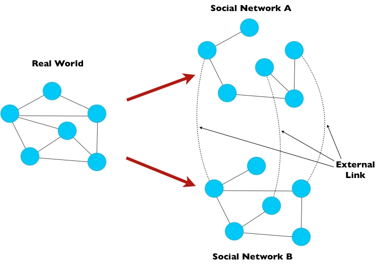
Figure 1: From the real underlying social network, the model generates two random realizations of it, A and B, and some identification links for a subset of the users across the two realizations

For the two imperfect copies of the underlying network we assume that $G_{1}$ (respectively $G_{2}$) is created by selecting each edge $e\in E$ of the original graph $G(V,E)$ independently with a fixed probability $s_{1}$ (resp. $s_{2}$) (See Figure 1.) In the real world, edges/relationships are not selected truly independently, but this serves as a reasonable approximation for observed networks. In fact, a similar model has been previously considered by [26], which also produced experimental evidence from an email network to support the independent random selection of edges. Another plausible mechanism for edge creation in social network is the cascade model, in which nodes are more likely to join a new network if more of their friends have joined it. Experimentally, we show that our algorithm performs even better in the cascade model than in the independent edge deletion model.

These two models are theoretically interesting and practically interesting [26]. Nevertheless, in some cases the analyzed social networks may differ in their scopes and so the group of friends that a user has in a social network can greatly differ from the group of friends that same user has in the other network. To capture this scenario in the experimental section, we also consider the Affiliation Network model [19] (in which users participate in a number of communities) as the underlying social network. For each of $G_{1},G_{2}$, and for each community, we keep or delete all the edges inside the community with constant probability. This highly correlated edge deletion process captures the fact that a user’s personal friends might be connected to her on one network, while her work colleagues are connected on the second network. We defer the detailed description of this experiment to Section 5.

Recall that the user identification problem, given only the graph information, is intractable in general graphs. Even the special case where $s_{1}=s_{2}=1$ (that is, no edges have been deleted) is equivalent to the well-studied Graph Isomorphism problem, for which no polynomial-time algorithm is known. Fortunately, in reality, there are additional sources of information which allow one to identify a subset of nodes across the two networks: For example, people can use the same email address to sign up on multiple websites. Users often explicitly connect their network accounts, for instance by posting a link to their Facebook profile page on Google+ or Twitter and vice versa. To model this, we assume that there is a set of users/nodes explicitly linked across the two networks $G_{1},G_{2}$. More formally, there is a linking probability $l$ (typically, $l$ is a small constant) and each node in $V$ is linked across the networks independently with probability $l$. (In real networks, nodes may be linked with differing probabilities, but high-degree nodes / celebrities may be more likely to connect their accounts and engage in cross-network promotions; this would be more likely to help our algorithm, since low-degree nodes are less valuable as seeds because they help identify only a small number of neighbors. In the experiments of [23], the authors explicitly consider high-degree nodes as seeds in the real-world experiments.)

In Section 3.2 below, we present a natural algorithm to solve the user identification problem with a set of linked nodes, and discuss some of its properties. Then, in Section 4, we prove that this algorithm performs well on several well-established network models. In Section 5, we show that the algorithm also works very well in practice, by examining its performance on real-world networks.

3.2 The Algorithm

To solve the user identification problem, we design a local distributed algorithm that uses only structural information about the graphs to expand the initial set of links into a mapping/identification of a large fraction of the nodes in the two networks.

Before describing the algorithm, we introduce a useful definition.

Definition 1.

A pair of nodes $(u_{1},u_{2})$ with $u_{1}\in G_{1},u_{2}\in G_{2}$ is said to be a similarity witness for a pair $(v_{1},v_{2})$ with $v_{1}\in G_{1},v_{2}\in G_{2}$ if $u_{1}\in N_{1}(v_{1}),u_{2}\in N_{2}(v_{2})$ and $u_{1}$ has been linked to / identified with $u_{2}$.

Here, $N_{1}(v_{1})$ denotes the neighborhood of $v_{1}$ in $G_{1}$, and similarly $N_{2}(v_{2})$ denotes the neighborhood of $v_{2}$ in $G_{2}$.

Roughly speaking, in each phase of the algorithm, every pair of nodes (one from each network) computes an similarity score that is equal to the number of similarity witnesses they have. We then create a link between two nodes $v_{1}$ and $v_{2}$ if $v_{2}$ is the node in $G_{2}$ with maximum similarity score to $v_{1}$ and vice versa. We then use the newly generated set of links as input to the next phase of the algorithm.

A possible risk of this algorithm is that in early phases, when few nodes in the network have been linked, low-degree nodes could be mis-matched. To avoid this (improving precision), in the $i$th phase, we only allow nodes of degree roughly $D/2^{i}$ and above to be matched, where $D$ is a parameter related to the largest node degree. Thus, in the first phase, we match only the nodes of very high degree, and in subsequent phases, we gradually decrease the degree threshold required for matching. In the experimental section we will show in fact that this simple step is very effective, reducing the error rate by more than $33\%$. We summarize the algorithm, that we called User-Matching, as follows:

Input: $G_{1}(V,E_{1}),G_{2}(V,E_{2}),L$ a set of initial identification links across the networks, $D$ the maximum degree in the graph a minimum matching score $T$ and a specified number of iteration $k$. Output: A larger set of identification links across the networks. Algorithm: For $i=1,\dots,k$ For $j=\log D,\dots,1$ For all the pairs $(u,v)$ with $u\in G_{1}$ and $v\in G_{2}$ and such that $d_{G_{1}}(u)\geq 2^{j}$ and $d_{G_{2}}(v)\geq 2^{j}$ Assign to $(u,v)$ a score equal to the number of similarity witnesses between $u$ and $v$ If $(u,v)$ is the pair with highest score in which either $u$ or $v$ appear and the score is above $T$ add $(u,v)$ to $L$. Output $L$

Where $d_{G_{i}}(u)$ is the degree of node $u$ in $G_{i}$. Note that the internal for loop can be implemented efficiently with $4$ consecutive rounds of MapReduce, so the total running time would consist of $O(k\log D)$ MapReductions. In the experiments, we note that even for a small constant $k$ ($1$ or $2$), the algorithm returns very interesting results. The optimal choice of threshold $T$ depends on the desired precision/recall tradeoff; higher choices of T improve precision, but in our experiments, we note that $T=2$ or $3$ is sufficient for very high precision.

4 Theoretical Results

In this section we formally analyze the performance of our algorithm on two network models. In particular, we explain why our simple algorithm should be effective on real social networks. The core idea of the proofs and the algorithm is to leverage high degree nodes to discover all the possible mapping between users. In fact, as we show here theoretically and later experimentally, high degree nodes are easy to detect. Once we are able to detect the high degree nodes, most low degree nodes can be identified using this information.

We start with the Erdős-Rényi (Random) Graph model [11] to warm up with the proofs, and to explore the intuition behind the algorithm. Then we move to our main theoretical results, for the Preferential Attachment Model. For simplicity of exposition, we assume throughout this section that $s_{1}=s_{2}=s$; this does not change the proofs in any material detail.

4.1 Warm up: Random Graphs

In this section, we prove that if the underlying ‘true’ network is a random graph generated from the Erdős-Rényi model (also known as $G(n,p)$), our algorithm identifies almost all nodes in the network with high probability.

Formally, in the $G(n,p)$ model, we start with an empty graph on $n$ nodes, and insert each of the $\binom{n}{2}$ possible edges independently with probability $p$. We assume that $p<1/6$; in fact, any constant probability results in graphs which are much denser than any social network. Let $G$ be a graph generated by this process; given this underlying network $G$, we now construct two partial realizations $G_{1},G_{2}$ as described by our model of Section 3.

We note that the probability a specific edge exists in $G_{1}$ or $G_{2}$ is $ps$. Also, if $nps$ is less than $(1-\varepsilon)\log n$ for $\varepsilon>0$, the graphs $G_{1}$ and $G_{2}$ are not connected w.h.p. [11]. Therefore, we assume that $nps>c\log n$ for some constant $c$.

In the following we identify the nodes in $G_{1}$ with $u_{1},\dots,u_{n}$ and the nodes in $G_{2}$ with $v_{1},\dots,v_{n}$, where nodes $u_{i}$ and $v_{i}$ correspond to the same node $i$ in $G$. In the first phase, the expected number of similarity witnesses for a pair $(u_{i},v_{i})$ is $(n-1)ps^{2}\cdot l$. This follows because the expected number of neighbors of $i$ in $G$ is $(n-1)p$, the probability that the edge to a given neighbor survives in both $G_{1}$ and $G_{2}$ is $s^{2}$, and the probability that it is initially linked is $l$. On the other hand, the expected number of similarity witnesses for a pair $(u_{i},v_{j})$, with $i\neq j$ is $(n-2)p^{2}s^{2}\cdot l$; the additional factor of $p$ is because a given other node must have an edge to both $i$ and $j$, which occurs with probability $p^{2}$. Thus, there is a factor of $p$ difference between the expected number of similarity witnesses a node $u_{i}$ has with its true match $v_{i}$ and with some other node $v_{j}$, with $i\neq j$. The main intuition is that this factor of $p<1$ is enough to ensure the correctness of algorithm. We prove this by separately considering two cases: If $p$ is sufficiently large, the expected number of similarity witnesses is large, and we can apply a concentration bound. On the other hand, if $p$ is small, $np^{2}s^{2}$ is so small that the expected number of similarity witnesses is almost negligible.

We start by proving that in the first case there is always a gap between a real and a false match.

Theorem 1.

If $(n-2)ps^{2}l\geq 24\log n$ (that is, $p>\frac{24}{s^{2}l}\frac{\log n}{n-2}$), w.h.p. the number of first-phase similarity witnesses between $u_{i}$ and $v_{i}$ is at least $(n-1)ps^{2}l/2$. The number of first-phase similarity witnesses between $u_{i}$ and $v_{j}$, with $i\neq j$ is w.h.p. at most $(n-2)ps^{2}l/2$.

Proof.

We prove both parts of the lemma using Chernoff Bounds (see, for instance, [10]).

Let consider a pair for node $j$. Let $Y_{i}$ be a r.v. such that $Y_{i}=1$ if node $u_{i}\in N_{1}(u_{j})$ and $v_{i}\in N_{2}(v_{j})$, and if $(u_{i},v_{i})\in L$, where $L$ is the initial seed of links across $G_{1}$ and $G_{2}$. Then, we have $Pr[Y_{1}=1]=ps^{2}l$. If $Y=\sum_{i=1}^{n-1}Y_{i}$, the Chernoff bound implies that $Pr[Y<(1-\delta)E[Y]]\leq e^{-E[Y]\delta^{2}/2}$. That is,

$$Pr\left[Y<\frac{1}{2}(n-1)ps^{2}l\right]\leq e^{-E[Y]/8}<e^{-3\log n}=1/n^{3}$$

Now, taking the union bound over the $n$ nodes in $G$, w.h.p. every node has the desired number of first-phase similarity witnesses with its copy.

To prove the second part, suppose w.l.o.g. that we are considering the number of first-phase similarity witnesses between $u_{i}$ and $v_{j}$, with $i\neq j$. Let $Y_{i}=1$ if node $u_{z}\in N_{1}(u_{i})$ and $v_{z}\in N_{2}(v_{j})$, and if $(u_{z},v_{x})\in L$. If $Y=\sum_{i=1}^{n-2}Y_{i}$, the Chernoff bound implies that $Pr[Y>(1+\delta)E[Y]]\leq e^{-E[Y]\delta^{2}/4}$. That is,

$$Pr\left[Y>\frac{1}{2p}(n-2)p^{2}s^{2}l=\frac{(n-2)ps^{2}l}{2}\right]\leq e^{-E[Y]({1\over 2p}-1)^{2}/4}$$

$$=e^{-2p({1\over 2p}-1)^{2}3\log n}\leq 1/n^{3}$$

where the last inequality comes from the fact that $p<1/6$. Taking the union bound over all $n(n-1)$ unordered pairs of nodes $u_{i},v_{j}$ gives the fact that w.h.p., every pair of different nodes does not have too many similarity witnesses. ∎

The theorem above implies that when $p$ is sufficiently large, there is a gap between the number of similarity witnesses of pairs of nodes that correspond to the same node and a pair of nodes that do not correspond to the same node. Thus the first-phase similarity witnesses are enough to completely distinguish between the correct copy of a node and possible incorrect matches.

It remains only to consider the case when $p$ is smaller than the bound required for Theorem 1. This requires the following useful lemma.

Lemma 2.

Let $B$ be a Bernoulli random variable, which is 1 with probability at most $x$, and 0 otherwise. In $k$ independent trials, let $B_{i}$ denote the outcome of the $i$th trial, and let $B(k)=\sum_{i=1}^{k}B_{i}$: If $kx$ is $o(1)$, the probability that $B(k)$ is greater than $2$ is at most $k^{3}x^{3}/6+o(k^{3}x^{3})$.

Proof.

The probability that $B(k)$ is at most 2 is given by: $(1-x)^{k}+kx\cdot(1-x)^{k-1}+\binom{k}{2}x^{2}\cdot(1-x)^{k-2}$. Using the Taylor series expansion for $(1-x)^{k-2}$, this is at most $1-k^{3}x^{3}/6-o(k^{3}x^{3})$. ∎

When we run our algorithm on a graph drawn from $G(n,p)$, we set the minimum matching threshold to be $3$.

Lemma 3.

If $p\leq\frac{24}{s^{2}l}\frac{\log n}{n-2}$, w.h.p., algorithm User-Matching never incorrectly matches nodes $u_{i}$ and $v_{j}$ with $i\neq j$.

Proof.

Suppose for contradiction the algorithm does incorrectly match two such nodes, and consider the first time this occurs. We use Lemma 2 above. Let $B_{z}$ denote the event that the vertex $z$ is a similarity witness for $u_{i}$ and $v_{j}$.

In order for $B_{z}$ to have occurred, we must have $u_{z}$ in $N_{1}(U_{i})$ and $v_{z}$ in $N_{2}(v_{j})$ and $(u_{z},v_{z})\in L$. The probability that $B_{z}=1$ is therefore at most $p^{2}s^{2}$. Note that each $B_{z}$ is independent of the others, and that there are $n-2$ such events. As $p$ is $O(\log n/n)$, the conditions of Lemma 2 apply, and hence the probability that more than 2 such events occur is at most $(n-2)^{3}p^{6}s^{6}$. But $p$ is $O(\log n/n)$, and hence this event occurs with probability at most $O(\log^{6}n/n^{3})$. Taking the union bound over all $n(n-1)$ unordered pairs of nodes $u_{i},v_{j}$ gives the fact that w.h.p., not more than 2 similarity witnesses can exist for any such pair. But since the minimum matching threshold for our algorithm is $3$, the algorithm does not incorrectly match this pair, contradicting our original assumption. ∎

Having proved that our algorithm does not make errors, we now show that it identifies most of the graph.

Theorem 4.

Our algorithm identifies $1-o(1)$ fraction of the nodes w.h.p.

Proof.

Note that the probability that a node is identified is $1-o(1)$ by the Chernoff bound because in expectation it has $\Omega(\log n)$ similarity witnesses. So in expectation, we identify $1-o(1)$ fraction of the nodes. Furthermore, by applying the method of bounded difference [10] (each node affects the final result at most by $1$), we get that the result holds also with high probability. ∎

4.2 Preferential Attachment

The preferential attachment model was introduced by Barabási and Albert in [5]. In this paper we consider the formal definition of the model described in [6].

Definition 2.

[PA model]. Let $G_{n}^{m}$, $m$ being a fixed parameter, be defined inductively as follows:

• $G_{1}^{m}$ consists of a single vertex with $m$ self-loops.

• $G_{n}^{m}$ is built from $G_{n-1}^{m}$ by adding a new node $u$ together with $m$ edges $e_{u}^{1}=(u,v_{1}),\ldots,e_{u}^{m}=(u,v_{m})$ inserted one after the other in this order. Let $M_{i}$ be the sum of the degrees of all the nodes when the edge $e_{u}^{i}$ is added. The endpoint $v_{i}$ is selected with probability $\frac{deg(v_{i})}{M_{i}+1}$, with the exception of node $u$, which is selected with probability $\frac{d(u)+1}{M_{i}+1}$.

The PA model is the most celebrated model for social networks. Unlike the Erdős-Rényi model, in which all nodes have roughly the same degree, PA graphs have a degree distribution that more accurately resembles the skew degree distribution seen in real social networks. Though more evolved models of social networks have been recently introduced, we focus on the PA model here because it clearly illustrates why our algorithm works in practice. Note that the power-law distribution of the model complicates our proofs, as the overwhelming majority of nodes only have constant degree ($\leq 2m$), and so we can no longer simply apply concentration bounds to obtain results that hold w.h.p. For a (small) constant fraction of the nodes $u$, there does not exist any node $z$ such that $u_{z}\in N_{1}(u_{i})$ and $v_{z}\in N_{2}(v_{i})$; we cannot hope to identify these nodes, as they have no neighbors “in common” on the two networks. In fact, if $m=4$ and $s=1/2$, roughly $30\%$ of nodes of “true” degree $m$ will be in this situation. Therefore, to be able to identify a reasonable fraction of the nodes, one needs $m$ to be at least a reasonably large constant; this is not a serious constraint, as the median friend count on Facebook, for instance, is over 100. In our experimental section, we show that our algorithm is effective even with smaller $m$.

We now outline our overall approach to identify nodes across two PA graphs. In Lemma 11, we argue that for the nodes of very high degree, their neighborhoods are different enough that we can apply concentration arguments and uniquely identify them. For nodes of intermediate degree ($\log^{3}n$) and less, we argue in Lemma 10 that two distinct nodes of such degree are very unlikely to have more than 8 neighbors in common. Thus, running our algorithm with a minimum matching threshold of 9 guarantees that there are no mistakes. Finally, we prove in Lemma 12 that when we run the algorithm iteratively, the high-degree nodes help us identify many other nodes, these nodes together with the high-degree nodes in turn help us identify more, and so on: Eventually, the probability that any given node is unidentified is less than a small constant, which implies that we correctly identify a large fraction of the nodes.

Interestingly, we notice in our experiments that on real networks, the algorithm has the same behavior as on PA graphs. In fact, as we will discuss later, the algorithm is always able to identify high-degree/important nodes and then, using this information, identify the rest of the graph.

Technical Results: The first of the three main lemmas we need, Lemma 11, states that we can identify all of the high-degree nodes correctly. To prove this, we need a few technical results. These results say that all nodes of high degree join the network early, and continue to increase their degree significantly throughout the process; this helps us show that high-degree nodes do not share too many neighbors.

4.2.1 High degree nodes are early-birds

Here we will prove formally that the nodes of degree $\Omega(\log^{2}n)$ join the network very early; this will be useful to show that two high degree nodes do not share too many neighbors.

Lemma 5.

Let $G_{n}^{m}$ be the preferential attachment graph obtained after $n$ steps. Then for any node $v$ inserted after time $\psi n$, for any constant $\psi>0$, $d_{n}(v)\in o(log^{2}n)$ with high probability, where $d_{n}(v)$ is the degree of nodes $v$ at time $n$.

Proof.

It is possible to prove that such nodes have expected constant degree, but unfortunately, it is not trivial to get a high probability result from this observation because of the inherent dependencies that are present in the preferential attachment model. For this reason we will not prove the statement directly, but we will take a short detour inspired by the proof in [18]. In particular we will first break the interval in a constant number of small intervals. Then we will show that in each interval the degree of $v$ will increase by at most $O(\log n)$ with high probability. Thus we will be able to conclude that at the end of the process the total degree of $v$ is at most $O(\log n)$(recall that we only have a constant number of interval).

As mentioned above we analyze the evolution of the degree of $v$ in the interval $\psi n$ to $n$ by splitting this interval in a constant number of segments of length $\lambda n$, for some constant $\lambda>0$ to be fixed later. Now we can focus on what happens to the degree of $v$ in the interval $(t,\cdot\lambda n+t]$ if $d_{t}(v)\leq C\log n$, for some constant $C\geq 1$ and $t\geq\psi n$. Note that if we can prove that $d_{\lambda n+t}\leq C^{\prime}\log n$, for some constant $C^{\prime}\geq 0$ with probability $1-o\left(n^{-2}\right)$, we can then finish the proof by the arguments presented in the previous paragraph.

In order to prove this, we will take a small detour to avoid the dependencies in the preferential attachment model. More specifically, we will first show that this is true with high probability for a random variable $X$ for which it is easy to get the concentration result. Then we will prove that the random variable $X$ stochastically dominates the increase in the degree of $v$. Thus the result will follow.

Now, let us define $X$ as the number of heads that we get when we toss a coin which gives head with probability $\frac{C^{\prime}\log n}{t}$ for $\lambda n$ times, for some constant $C^{\prime}\geq 13C$. It is possible to see that:

$$E[X]=\frac{C^{\prime}\log n}{t}\lambda n\leq\frac{C^{\prime}\log n}{\psi n}\lambda n\leq\frac{C^{\prime}\lambda\log n}{\psi}$$

Now we fix $\lambda=\frac{\psi}{100}$ and we use the Chernoff bound to get the following result:

$$\Pr\left(X>\frac{C^{\prime}-C}{2}\log n\right) = \Pr\Bigg{(}X>\left(\frac{100(C^{\prime}-C)}{2C^{\prime}}\right)E[X]\Bigg{)}$$

$$\leq 2^{-\frac{C^{\prime}}{100}\log n\left(\frac{100(C^{\prime}-C)}{2C^{\prime}}\right)}$$

$$\leq 2^{-\left(\frac{(6C^{\prime})}{13}\log n\right)}$$

$$\leq 2^{-6\log n}\in O\left(n^{-3}\right)$$

So we know that the value of $X$ is bounded by $\frac{C^{\prime}-C}{2}\log n$ with probability $O\left(n^{-3}\right)$. Now, note that until the degree of $v$ is less than $C^{\prime}\log n$ the probability that $v$ increases its degree in the next step is stochastically dominated by the probability that we get an head when we toss a coin which gives head with probability $\frac{C^{\prime}\log n}{t}$. To conclude our algorithm we study the probability that $v$ become of degree $\frac{C^{\prime}\log n}{t}$ precisely at time $t\leq t^{*}\leq\lambda n$. Note that until time $t^{*}$ $v$ has degree smaller than $\frac{C^{\prime}\log n}{t}$ and so it is dominated by the coin. But we already know that when we toss such a coin at most $\lambda n$ times the probability of getting $\frac{C^{\prime}-C}{2}\log n$ heads is in $O\left(n^{-3}\right)$. Thus for any $t\leq t^{*}\leq\lambda n$ the probability that $v$ reach degree $C^{\prime}\log n$ at time $t^{*}$ is $O(n^{-3})$. Thus by using the union bound on all the possible $t^{*}$, $v$ will get to degree $C^{\prime}\log n$ with probability $O(n^{-2})$.

At this point we can finish the proof by taking the union bound on all the segments(recall that they are constant) $(\psi n,\psi+\lambda n],(\psi+\lambda n,\psi n+2\lambda],\cdots$ and on the number of nodes and we get that all the nodes that join the network after time $\psi n$ have degree that is upper bounded by $C^{\prime\prime}\log n$ for some constant $C^{\prime\prime}\geq 0$ with probability $O(n^{-1})$. ∎

4.2.2 The rich get richer

In this section we study another fundamental property of the preferential attachment, which is that nodes with degree bigger than $\log^{2}n$ continue to increase their degree significantly throughout the process. More formally:

Lemma 6.

Let $G_{n}^{m}$ be the preferential attachment graph obtained after $n$ steps. Then with high probability for any node $v$ of degree $d\geq\log^{2}n$ and for any fixed constant $\epsilon\geq 0$, a $\frac{1}{3}$ fraction of the neighbors of $v$ joined the graph after time $\epsilon n$.

Proof.

By Lemma 5 above, we know that $v$ joined the network before time $\epsilon n$ for any fixed constant $\epsilon\geq 0$. Now we consider two cases. In the first, $d_{\epsilon n}(v)\leq\frac{1}{2}\log^{2}n$, in which case the statement is true because the final degree is bigger than $\log^{2}n$. Otherwise, we have that $d_{\epsilon n}(v)>\frac{1}{2}\log^{2}n$, in this case the probability that $v$ increase its degree at every time step after $\epsilon n$ dominates the probability that a toss of a biased coin which gives head with probability $\frac{\log^{2}n}{2mn}$ comes up head. Now consider the random variable $X$ that counts the number of heads when we toss a coin that lands head with probability $\frac{\log^{2}n}{2mn}$ for $(1-\epsilon)mn$ times. The expected value of $X$ is:

$$E[X]=\frac{\log^{2}n}{2mn}(1-\epsilon)mn=\frac{1-\epsilon}{2}\log^{2}n$$

Thus using the Chernoff bound:

$$\Pr\left(X\leq\frac{1-2\epsilon}{2}\log^{2}n\right) \leq exp\left(-\frac{1}{2}\left(1-\frac{\epsilon}{1-\epsilon}\right)\log^{2}n\right)$$

$$\in O(n^{-2})$$

Thus with probability $O(1-n^{-2})$ $X$ is bigger that $\frac{1-2\epsilon}{2}\log^{2}n$ but as mentioned before the increase in the degree of $v$ stochastically dominates $X$. Thus taking the union bound on all the possible $v$ we get that the statement holds with probability equal to $O(1-n^{-1})$. Thus the claim follows. ∎

4.2.3 First-mover advantage

Lemma 7.

Let $G_{n}^{m}$ be the preferential attachment graph obtained after $n$ steps. Then with high probability all the nodes that join the network before time $n^{0.3}$ have degree at least $\log^{3}n$.

Proof.

To prove this theorem we will use some results from [9], but before we need to introduce another model equivalent to the preferential attachment. In this new process instead of constructing $G_{n}^{m}$, we first construct $G_{nm}^{1}$ and then we collapse the vertices $1,\cdots,m$ to construct the first vertex, the vertex between $m+1,\cdots 2m$ to construct the second vertex and so on so for. It is not hard to see that this new model is equivalent to the preferential attachment. Now we can prove our technical theorem.

Now we can state two useful equation from the proof of Lemma 6 in [9]. Consider the model $G_{1}^{nm}$. Let $D_{k}=d_{nm}(v_{1})+d_{nm}(v_{2})+\cdots+d_{nm}(v_{k})$, where $d_{nm}(v_{i})$ is the degree of a node inserted at time $i$ at time $nm$. Then $k\geq 1$ we have:

$$\Pr\left(|D_{k}-2\sqrt{kmn}|\geq 3\sqrt{mn\log(mn)}\right)\leq(mn)^{-2}$$ (1)

From the same paper we also have that if $0\leq d\leq mn-k-s$, we can derive from equation (23) that

$$\Pr(d_{n}(v_{k+1})=d+1|D_{k}-2k=s)\leq\frac{s+d}{2N-2k-s-d}$$ (2)

From 1 we can derive that:

$$\Pr\left(D_{k}-2k\geq 3\sqrt{mn\log(mn)}+2\sqrt{kmn}-2k\right)\leq(mn)^{-2}$$

$$\Pr\left(D_{k}-2k\geq 5\sqrt{kmn\log(mn)}\right)\leq(mn)^{-2}$$

Thus we get that:

$$\Pr(d_{n}(v_{k+1})<\log^{3}n)=\sum_{0}^{\log^{3}n-1}\Pr(d_{n}(v_{k+1})=i)$$

$$\leq \Pr\left(D_{k}-2k\geq 3\sqrt{mn\log(mn)}+2\sqrt{kmn}-2k\right)$$

$$+ \sum_{i=0}^{\log^{3}n-1}\sum_{j=0}^{5\sqrt{kmn\log(mn)}}\Big{(}\Pr\left(D_{k}-2k=j\right)$$

$$\Pr(d_{n}(v_{k+1})=i|D_{k}-2k=j)\Big{)}$$

$$\leq (mn)^{-2}+\sum_{i=0}^{\log^{3}n-1}\Pr\Big{(}d_{n}(v_{k+1})=i|D_{k}-2k$$

$$=5\sqrt{mn\log(mn)}\Big{)}$$

$$\leq (mn)^{-2}+\sum_{i=0}^{\log^{3}n-1}\frac{5\sqrt{mn\log(mn)}+i-1}{2mn-2k-5\sqrt{mn\log(mn)}-i+1}$$

$$\in O\left(\frac{\log^{4}(n)}{\sqrt{n}}\right)$$

where we assumed that $k\in O\left(n^{\frac{1}{3}}\right)$.

So now by union bounding on the first $mn^{0.3}$ nodes we obtain that with high probability in $G_{1}^{nm}$ all the nodes have degree bigger than $\log^{2}n$. But this implies in turn the statement of the theorem by construction of $G_{1}^{nm}$ . ∎

4.2.4 Handling product of generalized harmonic

Lemma 8.

Let $a$ and $b$ be constant greater than $0$. Then:

$$\sum_{i=n^{a}}^{n^{b}-2}\sum_{j>i}^{n^{b}-1}\sum_{z>j}^{n^{b}}\frac{1}{i^{2}j^{2}z^{2}}\in O\left(\frac{1}{n^{3a}}\right)$$

Proof.

Recall that $\sum_{k=x}^{y}\frac{1}{k^{2}}\in\Theta(\frac{1}{x}-\frac{1}{y})$. Then

$$\sum_{i=n^{a}}^{n^{b}-2}\sum_{j>i}^{n^{b}-1}\sum_{z>j}^{n^{b}}\frac{1}{i^{2}j^{2}z^{2}} = \sum_{i=n^{a}}^{n^{b}-2}\frac{1}{i^{2}}\sum_{j>i}^{n^{b}-1}\frac{1}{j^{2}}\sum_{z>j}^{n^{b}}\frac{1}{z^{2}}$$

$$\in \Theta(\frac{1}{n^{a}}-\frac{1}{n^{b}})\Theta(\frac{1}{n^{a}}-\frac{1}{n^{b}})\Theta(\frac{1}{n^{a}}-\frac{1}{n^{b}})$$

$$\in O\left(\frac{1}{n^{3a}}\right)$$

∎

Completing the Proof: We now use the technical lemmas above to complete our proof for the preferential attachment model.

Lemma 9.

For a node $u$ with degree $d$, the probability that it is incident to a node arriving at time $i$ is at most $\max\{d,\log^{3}n\}/(i-1)$ w.h.p.

Proof.

If node $i$ arrives after $u$, the probability that $i$ is adjacent to $u$ is at most the given value, since there are $m(i-1)$ edges existing in the graph already, and we take the union bound over the $m$ edges incident to $i$. If $i$ arrives before $u$, let $t$ denote the time at which $u$ arrives. From Lemma 6 of [9], the degree of $i$ at t is at most $\sqrt{t}{i}\log^{3}n$ w.h.p.. But there are $(t-1)m$ edges already in the graph at this time, and since $u$ has $m$ edges incident to it, the probability that one of them is incident to $i$ is at most $\log^{3}n\frac{\sqrt{t}}{\sqrt{i}(t-1)}\leq\log^{3}n/(i-1)$. ∎

Lemma 10.

W.h.p, for any pair of nodes $u,v$ of degree $<\log^{3}n$, $|N(u)\cap N(v)|\leq 8$.

Proof.

From Lemma 7, nodes $u$ and $v$ must have arrived after time $t=n^{0.3}$. Let $a,b$ be constants such that $0.3<a<b<1$ and $b\leq 3/2a-\varepsilon$ for some constant $\varepsilon>0$. We first show that the probability that any two nodes $u,v$ with degree less than $\log^{3}n$ and arriving before time $n^{b}$ have $3$ or more common neighbors between $n^{a}$ and $n^{b}$ is at most $n^{-\varepsilon}$. This implies that, setting $a$ to $0.3$, nodes $u$ and $v$ have at most 2 neighbors between $n^{a}$ and $n^{3a/2-\varepsilon}$, at most 2 between $n^{3a/2-\varepsilon}$ and $n^{9a/4}$, and at most 2 between $n^{9a/4}$ and $n^{27a/8}>n$, for a total of 6 overall. Similarly, we show that $u$ and $v$ have at most 2 neighbors arriving before $n^{0.3}$, which completes the lemma.

From Lemma 9 above, the probability that a node arriving at time $i$ is incident to $u$ and $v$ is at most $(\log^{3}n/(i-1))^{2}$. (The events are not independent, but they are negatively correlated.) The probability that 3 nodes $i,j,k$ are all incident to both $u$ and $v$, then, is at most $(\log^{3}n)^{6}/((i-1)(j-1)(k-1))^{2}$. Therefore, for a fixed $u,v$, the probability that some 3 nodes are adjacent to $u$ and $v$ is at most:

$$\log^{18}n\sum_{i=n^{a}}^{n^{b}}\sum_{j=n^{a}}^{n^{b}}\sum_{k=n^{a}}^{n^{b}}\frac{1}{\left((i-1)(j-1)(k-1)\right)^{2}}$$

$$\leq \log^{18}n\left(\frac{1}{n^{a}}-\frac{1}{n^{b}}\right)^{3}$$

There are at most $n^{b}$ choices for each of $u$ and $v$; taking the union bound, the probability that any pair $u$, $v$ have 3 or more neighbors in common is at most $n^{2b-3a}\log^{18}n=n^{-2\varepsilon}\log^{18}n$. ∎

So, by setting the matching threshold to $9$, the algorithm never makes errors; we now prove that it actually detects a lot of good new links.

Lemma 11.

The algorithm successfully identifies any node of degree $\geq 4\log^{2}n/(s^{2}l)$.

Proof.

For any node $v$ of degree $d(v)\geq 4\log^{2}n/(s^{2}l)$, the expected number of similarity witnesses it has with its copy during the first phase is $d(v)s^{2}l$; using the Chernoff Bound, the probability that the number is less than $7/8$ of its expectation is at most $\exp(-d(v)s^{2}l/128)\leq\exp(-\log^{2}n/32)=\frac{1}{n^{\log n/32}}$. Therefore, with very high probability, every node $v$ of degree $d(v)$ has at least $7/8\cdot d(v)s^{2}l$ first-phase similarity witnesses with its copy.

On the other hand, how many similarity witnesses can node $v$ have with a copy of a different node $u$? Fix $\varepsilon>0$, and first consider potential similarity witnesses that arrive before time $t=\varepsilon n$; later, we consider those that arrive after this time. From Lemma 6, we have $d_{t}(v)\leq(2/3+\varepsilon)d(v)$. Even if all of these neighbors of $v$ are also incident to $u$, the expected number of similarity witnesses for $(u,v)$ is at most $d_{t}(v)s^{2}l$. Now consider the neighbors of $v$ that arrive after time $\varepsilon n$. Each of these nodes is a neighbor of $u$ with probability $\leq d(u)/(2m\varepsilon n)$. But $d(u)\leq\tilde{O}(\sqrt{n})$, and hence each of the neighbors of $v$ is a neighbor of $u$ with probability $o(1/n^{1/2-\delta})$. Therefore, the expected number of similarity witnesses for $(u,v)$ among these nodes is at most $d(v)s^{2}l/n^{1/2-\delta}$. Therefore, the total expected number of similarity witnesses is at most $(2/3+\varepsilon)d(v)s^{2}l$. Again using the Chernoff Bound, the probability that this is at least $7/8\cdot d(v)s^{2}l$ is at most $\exp(-3/4d(v)s^{2}l\cdot/64)=\exp(-3\log^{2}n/64)$, which is at most $\frac{1}{n^{3\log n/64}}$.

To conclude, we showed that with very high probability, a high-degree node $v$ has at least $7/8\cdot d(v)s^{2}l$ first-phase similarity witnesses with its copy, and has fewer than this number of witnesses to the copy of any other node. Therefore, our algorithm correctly identifies all high-degree nodes. ∎

From the two preceding lemmas, we identify all the high-degree nodes, and make no mistakes on the low-degree nodes. It therefore remains only to show that we have a good success probability for the low-degree nodes. In the lemma below, we show this when $ms^{2}\geq 22$. We note that one still obtains good results even with a higher or lower value of $ms^{2}$, but it appears difficult to obtain a simple closed-form expression for the fraction of identified nodes. For ease of exposition, we present the case of $ms^{2}\geq 22$ here, but the proof generalizes in the obvious way.

Lemma 12.

Suppose $ms^{2}\geq 22$. Then, w.h.p., we successfully identify at least $97\%$ of the nodes.

Proof.

We have already seen that all high-degree nodes (those arriving before time $n^{0.3}$) are identified in the first phase of the algorithm. Note also that it never makes a mistake; it therefore remains only to identify the lower-degree nodes. We describe a sequence of iterations in which we bound the probability of failing to identify other nodes.

Consider a sequence of roughly $n^{0.75}$ iterations, in each of which we analyze $n^{0.25}$ nodes. In particular, iteration $i$ contains all nodes that arrived between time $n^{0.3}+(i-1)n^{0.25}$ and time $n^{0.3}+i\cdot n^{0.25}$. We argue inductively that after iteration $i$, w.h.p. the fraction of nodes belonging to this iteration that are not identified is less than $0.03$, and the total fraction of degree incident to unidentified nodes is less than $0.08$. Since this is true for each $i$, we obtain the lemma.

The base case of nodes arriving before $n^{0.3}$ has already been handled. Now, note that during any iteration, the total degree incident to nodes of this iteration is at most $2mn^{0.25}\ll n^{0.3}$. Thus, when each node of this iteration, the probability that any of its $m$ edges is incident to another node of this iteration is less than $0.01$.

Consider any of the $m$ edges incident to a given node of this iteration. For each edge, we say it is good if it survives in both copies of the graph, and is incident to an identified node from a previous iteration. Thus, the probability that an edge is good is at least $s^{2}\cdot(0.99\times 0.92)$. Since $ms^{2}>22$, the expected number of good edges is greater than 20. The node will be identified if at least $8$ of its edges are good; applying the Chernoff bound, the probability that a given node is unidentified is at most $\exp(-3.606)<0.02717$.

Since this is true for each node of this iteration, regardless of the outcomes for previous nodes of the iteration, we can apply concentration inequalities even though the events are not independent. In particular, the number of identified nodes stochastically dominates the number of successes in $n^{0.25}$ independent Bernoulli trials with probability $1-\exp(-3.606)$ (see, for example, Theorem 1.2.17 of [21]). Again applying the Chernoff Bound, the probability that the fraction of unidentified nodes exceeds $0.03$ is at most $\exp(0.27n^{0.25}*0.01/4)$, which is negligible. To complete the induction, we need to show that the fraction of total degree incident to unidentified nodes is at most $0.08$. To observe this, note that the increase in degree is $2mn^{0.25}$; the unidentified fraction increases if the new nodes are unidentified (but we have seen the expected contribution here is at most $0.02717mn^{0.25}$), or if the “other” endpoint is another node of this iteration (at most $0.01mn^{0.25}$), or if the “other” endpoint is an unidentified node (in expectation, at most $0.08mn^{0.25}$). Again, a simple concentration argument completes the proof. ∎

5 Experiments

In this section we analyze the performance of our algorithm in different experimental settings. The main goal of this section is to answer the following eight questions:

• Are our theorems robust? Do our results depend on the constants that we use or are they more general?

• How does the algorithm scale on very large graphs?

• Does our algorithm work only for an underlying “real” network generated by a random process such as Preferential Attachment, or does it work for real social networks?

• How does the algorithm perform when the two networks to be matched are not generated by independently deleting edges, but by a different process like a cascade model?

• How does the algorithm perform when the two networks to be matched have different scopes? Is the algorithm robust to highly correlated edge deletion?

• Does our model capture reality well? In more realistic scenarios, with distinct but similar graphs, does the algorithm perform acceptably?

• How does our algorithm perform when the network is under attack? Can it still have high precision? Is it easy for an adversary to trick our algorithm?

• How important is it to bucket nodes by degree? How big is the impact on the algorithm’s precision? How does our algorithm compare with a simple algorithm that just counts the number of common neighbors?

To answer these eight questions, we designed $4$ different experiments using $6$ different publicly available data sets. These experiments are increasingly challenging for our algorithm, which performs well in all cases, showing its robustness. Before entering into the details of the experiments, we describe briefly the basic datasets used in the paper. We use synthetic random graphs generated by the Preferential Attachment [5], Affiliation Network [19], and RMAT [7] processes; we also consider an early snapshot of the Facebook graph [30], a snapshot of DBLP [1], the email network of Enron [16], a snapshot of Gowalla [8] (a social network with location information), and Wikipedia in two languages [2]. In Table 1 we report some general statistics on the networks.

Network	Number of nodes	Number of edges
PA [5]	1,000,000	20,000,000
RMAT24 [7]	8,871,645	520,757,402
RMAT26 [7]	32,803,311	2,103,850,648
RMAT28 [7]	121,228,778	8,472,338,793
AN [19]	60,026	8,069,546
Facebook [30]	63,731	1,545,686
DBLP [1]	4,388,906	2,778,941
Enron [16]	36,692	367,662
Gowalla [8]	196,591	950,327
French Wikipedia [2]	4,362,736	141,311,515
German Wikipedia [2]	2,851,252	81,467,497

Table 1: The original 11 datasets.

Robustness of our Theorems: To answer the first question, we use as an underlying graph the preferential attachment graph described above, with 1,000,000 nodes and $m=20$. We analyze the performance of our algorithm when we delete edges with probability $s=0.5$ and with different seed link probabilities. The main goal of this experiment is to show that the values of $m,s$ needed in our proof are only required for the calculations; the algorithm is effective even with much lower values. With the specified parameters, for the majority of nodes, the expected number of neighbors in the intersection of both graphs is $5$. Nevertheless, as shown in Figure 2, our algorithm performs remarkably well, making zero errors regardless of the seed link probability. Further, it recovers almost the entire graph. Unsurprisingly, lowering the threshold for our algorithm increases recall, but it is interesting to note that in this setting, it does not affect precision at all.

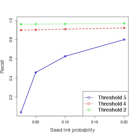
Figure 2: The number of corrected pairs detected with different threshold for the preferential attachment model with random deletion. The precision is not shown in the plot because it is always 100%.

Efficiency of our algorithms: Here we tested our algorithms with datasets of increasing size. In particular we generate 3 synthetic random graphs of increasing size using the RMAT random model. Then we use the three graphs as the underlying “real” networks and we generate $6$ graphs from them with edges surviving with probability $0.5$. Finally we analyze the running time of our algorithm with seed link probability equal to $0.10$. As shown in Table 2, using the same amount of resources, the running time of the algorithm increases by at most a factor $12.544$ between the smallest and the largest graph.

Network	Number of nodes	Relative running time
RMAT24	8871645	1
RMAT26	32803311	1.199
RMAT28	121228778	12.544

Table 2: The relative running time of the algorithm on three RMAT graphs as a function of numbers of nodes in the graph.

Robustness to other models of the underlying graph: For our third question, we move away from synthetic graphs, and consider the snapshots of Facebook and the Enron email networks as our initial underlying networks. For Facebook, edges survive either with probability $s=0.5$ or $s=0.75$, and we analyze performance of our algorithm with different seed link probabilities. For Enron, which is a much sparser network, we delete the edges with probability $s=0.5$ and analyze performance of our algorithm with seed link probability equal to $0.10$. The main goal of these experiments is to show that our algorithm has good performance even outside the boundary of our theoretical results even when the underlying network is not generated by a random model.

In the first experiment with Facebook, when edges survive with probability $0.75$, there are $63584$ nodes with degree at least $1$ in both networks. In the second, with edges surviving with probability $0.5$, there are $62854$ nodes with this property. In this case, the results are also very strong; see Table 3. Roughly $28\%$ of nodes have extremely low degree $(\leq 5)$, and so our algorithm cannot obtain recall as high as in the previous setting. However, we identify a very large fraction of the roughly $45250$ nodes with degree above $5$, and the precision is still remarkably good; in all cases, the error is well under $1\%$. Table 2 presents the full results for the harder case, with edge survival probability $0.5$. With edge survival probability $0.75$ (not shown in the table), performance is even better: At threshold $2$ and the lowest seed link probability of $5\%$, we correctly identify $46626$ nodes and incorrectly identify $20$, an error rate of well under $0.05\%$. In the case of Enron, the original email network is very sparse, with an average degree of approximately 20; this means that each copy has average degree roughly 10, which is much sparser than real social networks. Of the 36,692 original nodes, only 21,624 exist in the intersection of the two copies; over 18,000 of these have degree $\leq 5$, and the average degree is just over $4$. Still, with matching threshold $5$, we identify almost all the nodes of degree $5$ and above, and even in this very sparse graph, the error rate among newly identified nodes is $4.8\%$.

Pr	Threshold 5		Threshold 4		Threshold 2
	Good	Bad	Good	Bad	Good	Bad
$20\%$	23915	0	28527	53	41472	203
$10\%$	23832	49	32105	112	38752	213
$5\%$	11091	43	28602	118	36484	236

Pr	Threshold 5		Threshold 4		Threshold 3
	Good	Bad	Good	Bad	Good	Bad
$10\%$	3426	61	3549	90	3666	149

Table 3: Results for Facebook (Left) and Enron (Right) under the random deletion model. Pr denotes the seed link probability.

Robustness to different deletion models: We now turn our attention to the fourth question: How much do our results depend on the process by which the two copies are generated? To answer this, we analyze a different model where we generate the two copies of the underlying graph using the Independent Cascade Model of [12]. More specifically, we construct a graph starting from one seed node in the underlying social network and we add to the graph the neighbors of the node with probability $p=0.05$. Subsequently, every time we add a node, we consider all its neighbors and add each of them independently with probability $p=0.05$ (note that we can try to add a node to the graph multiple times).

The results in this cascade model are extremely good; in fact, for both Facebook and Enron we have $0$ errors; as shown for Facebook in Figure 3, we are able to identify almost all the nodes in the intersection of the two graphs (even at seed link prob. $5\%$, we identify $16,273/16533=98.4\%$).

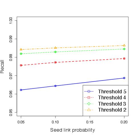
Figure 3: The number of corrected pairs detected with different threshold for the two Facebook graphs generated by the Independent Cascade Model. The plot does not show precision, since it is always 100%.

Robustness to correlated edge deletion: We now analyze one of the most challenging scenarios for our algorithm where, independently in the two realizations of the social network, we delete all or none of the edges in a community. For this purpose, we consider the Affiliation Networks model [19] as the underlying real network. In this model, a bipartite graph of users and interests is constructed using a preferential attachment-like process and then two users are connected in the network if and only if they share an interest (for the model details, refer to [19]). To generate the two copies in our experiment, we delete the interests independently in each copy with probability $0.25$, and then we generate the graph using only the surviving interests. Note that in this setting, the same node in the two realizations can have very different neighbors. Still, our algorithm has very high precision and recall, as shown in Table 4.

Pr	Threshold 4		Threshold 3		Threshold 2
	Good	Bad	Good	Bad	Good	Bad
$10\%$	54770	0	55863	0	55942	0

Table 4: Results for the Affiliation Networks model under correlated edge deletion probability.

Real world scenarios: Now we move to the most challenging case, where the two graphs are no longer generated by a mathematical process that makes 2 imperfect copies of the same underlying network. For this purpose, we conduct two types of experiments. First, we use the DBLP and the Gowalla datasets in which each edge is annotated with a time, and construct 2 networks by taking edges in disjoint time intervals. Then we consider the French- and German-language Wikipedia link graph.

From the co-authorship graph of DBLP, the first network is generated by considering only the publications written in even years, and the second is generated by considering only the publications written in odd years. Gowalla is a social network where each user could also check-in to a location (each check-in has an associated timestamp). Using this information we generate two Gowalla graphs; in the first graph, we have an edge between nodes if they are friends and if and only if they check-in to approximately the same location in an odd month. In the second, we have an edge between nodes if they are friends and if and only if they check-in in approximately the same location in an even month.

Note that for both DBLP and Gowalla, the two constructed graphs have a different set of nodes and edges, with correlations different from the previous independent deletion models. Nevertheless we will see that the intersection is big enough to retrieve a good part of the networks.

In DBLP, there are $380,129$ nodes in the intersection of the two graphs, but the considerable majority of them have extremely low degree. Over $310$K have degree less than $5$ in the intersection of the two graphs, and so again we cannot hope for extremely high recall. However, we do find considerably more nodes than in the input set. We start with a $10\%$ probability of seed links, resulting in $32087$ seeds; however, note that most of these have extremely low degree, and hence are not very useful. As shown in table 5, we have nearly $69,000$ nodes identified, with an error rate of under $4.17\%$. Note that we identify over half the nodes of degree at least $11$, and a considerably larger fraction of those with higher degree. We include a plot showing precision and recall for nodes of various degrees (Figure 4).

For Gowalla, there are 38103 nodes in the intersection of the two graphs, of which over 32K have degree $\leq 5$. We start with 3800 seeds, of which most are low-degree and hence not useful. We identify over 4000 of the (nearly 6000) nodes of degree above 5, with an error rate of $3.75\%$. See Table 5 and Figure 4 for more details.

Finally for a still more challenging scenario, we consider a case where the 2 networks do not have any common source, but yet may have some similarity in their structure. In particular, we consider the case of the French- and German-language Wikipedia sites, which have 4.36M and 2.85M nodes respectively. Wikipedia also maintains a set of inter-language links, which connect corresponding articles in a pair of languages; for French and German, there are 531710 links, corresponding to only $12.19\%$ of the French articles. The relatively small number of links illustrates the extent of the difference between the French and German networks. Starting with $10\%$ of the inter-language links as seeds, we are able to nearly triple the number of links (including finding a number of new links not in the input inter-language set), with an error rate of $17.5\%$ in new links. However, some of these mistakes are due to human errors in Wikipedia’s inter-language links, while others mistake French articles to closely connected German ones; for instance, we link the French article for Lee Harvey Oswald (the assassin of President Kennedy) to the German article on the assassination.

Pr	Threshold 5		Threshold 4		Threshold 2
	Good	Bad	Good	Bad	Good	Bad
10	42797	58	53026	641	68641	2985

Pr	Threshold 5		Threshold 4		Threshold 2
	Good	Bad	Good	Bad	Good	Bad
10	5520	29	5917	48	7931	155

Pr	Threshold 5		Threshold 3
	Good	Bad	Good	Bad
10	108343	9441	122740	14373

Table 5: Results for DBLP (Top Left), Gowala (Top Right), and Wikipedia (Bottom)

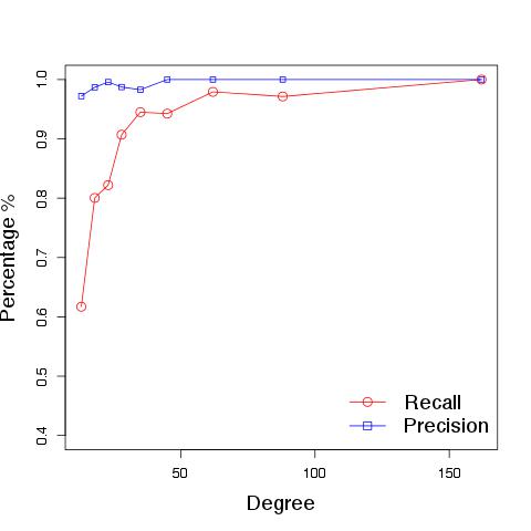
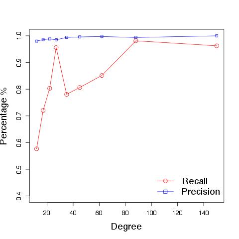
Figure 4: Precision and Recall vs. Degree Distribution for Gowala (left) and DBLP (right).

Robustness to attack: We now turn our attention to a very challenging question: what is the performance of our algorithm when the network is under attack? In order to answer this question, we again consider the Facebook network as the underlying social network, and from it we generate two realizations with edge probability $0.75$. Then, in order to simulate an attack, in each network for each node $v$ we create a malicious copy of it, $w$, and for each node $u$ connected to $v$ in the network (that is, $u\in N(v)$), we add the edge $(u,w)$ independently with probability $0.5$. Note that this is a very strong attack model (it assumes that users will accept a friend request from a ’fake’ friend with probability 0.5), and is designed to circumvent our matching algorithm. Nevertheless when we run our algorithm with seed link probability equal to $0.1$, and with threshold equal to $2$ we notice that we are still able to align a very large fraction of the two networks with just a few errors ($46955$ correct matches and $114$ wrong matches, out of $63731$ possible good matches).

Importance of degree bucketing, comparison with straightforward algorithm: We now consider our last question: How important is it to bucket nodes by degree? How big is the impact on the algorithm’s precision? How does our algorithm compare with a straightforward algorithm that just counts the number of common neighbors? To answer this question, we run a few experiments. First, we consider the Facebook graph with edge survival probability $0.5$ and seed link probability $5\%$, and we repeat the experiments again without using the degree bucketing and with threshold equal 1. In this case we observe that the number of bad matching increases by a factor of $50\%$ without any significant change in the number of good matchings.

Then we consider other two interesting scenarios: How does this simple algorithm perform on Facebook under attack? And how does it perform on matching Wikipedia pages? Those two experiments show two weaknesses of this simple algorithm. More precisely, in the first case the simple algorithm obtains $100\%$ precision but its recall is very low. It is indeed able to reconstruct less than half of the number of matches found by our algorithm (22346 vs 46955). On the other hand, the second setting shows that the precision of this simple algorithm can be very low. Specifically, the error rate of the algorithm is $27.87\%$, while our algorithm has error rate only $17.31\%$. In this second setting (for Wikipedia) the recall is also very low, less than $13.52\%$; there are 71854 correct matches, of which most (53174) are seed links, and 7216 wrong matches.

6 Conclusions

In this paper, we present the first provably good algorithm for social network reconciliation. We show that in well-studied models of social networks, we can identify almost the entire network, with no errors. Surprisingly, the perfect precision of our algorithm holds even experimentally in synthetic networks. For the more realistic data sets, we still identify a very large fraction of the nodes with very low error rates. Interesting directions for future work include extending our theoretical results to more network models and validating the algorithm on different and more realistic data sets.

Acknowledgements

We would like to thank Jon Kleinberg for useful discussions and Zoltán Gyöngyi for suggesting the problem.

References

- [1] Dblp. http://dblp.uni-trier.de/xml/.
- [2] Wikipedia dumps. http://dumps.wikimedia.org/.
- [3] F. Abel, N. Henze, E. Herder, and D. Krause. Interweaving public user profiles on the web. In UMAP 2010, pages 16–27.
- [4] L. Backstrom, C. Dwork, and J. Kleinberg. Wherefore art thou r3579x?: anonymized social networks, hidden patterns, and structural steganography. In WWW 2007, pages 181–190.
- [5] A.-L. Barabási and R. Albert. Emergence of scaling in random networks. Science, 286(5439):509–512, 1999.
- [6] B. Bollobás and O. Riordan. The diameter of a scale-free random graph. Combinatorica, 24(1):5–34, 2004.
- [7] D. Chakrabarti, Y. Zhan, and C. Faloutsos. R-mat: A recursive model for graph mining. In SDM 2004.
- [8] E. Cho, S. A. Myers, and J. Leskovec. Friendship and mobility: Friendship and mobility: User movement in location-based social networks. In KDD 2011, pages 1082–1090.
- [9] C. Cooper and A. Frieze. The cover time of the preferential attachment graph. Journal of Combinatorial Theory Series B, 97(2):269–290, 2007.
- [10] D. P. Dubhashi and A. Panconesi. Concentration of Measure for the Analysis of Randomized Algorithms. Cambridge University Press, 2009.
- [11] P. Erdős and A. Rényi. On Random Graphs I. Publ. Math. Debrecen, 6:290–297, 1959.
- [12] J. Goldenberg, B. Libai, and E. Muller. Talk of the network: Complex systems look at the underlying process of word-of-mouth. Marketing Letters 2001, pages 211–223.
- [13] M. Granovetter. The strength of weak ties: A network theory revisited. Sociological Theory, 1:201–233, 1983.
- [14] K. Henderson, B. Gallagher, L. Li, L. Akoglu, T. Eliassi-Rad, H. Tong, and C. Faloutsos. It’s who you know: graph mining using recursive structural features. In KDD 2011, pages 663–671.
- [15] J. Kleinberg. Navigation in a small world. Nature, 406(6798):845, 2000.
- [16] B. Klimmt and Y. Yang. Introducing the enron corpus. In CEAS conference 2004.
- [17] S. Labitzke, I. Taranu, and H. Hartenstein. What your friends tell others about you: Low cost linkability of social network profiles. In ACM Social Network Mining and Analysis 2011, pages 51–60.
- [18] S. Lattanzi. Algorithms and models for social networks. PhD thesis, Sapienza, 2011.
- [19] S. Lattanzi and D. Sivakumar. Affiliation networks. In STOC 2009, pages 427–434.
- [20] A. Malhotra, L. Totti, W. M. Jr., P. Kumaraguru, and V. Almeida. Studying user footprints in different online social networks. In CSOSN 2012, pages 1065–1070.
- [21] A. Műller and D. Stoyan. Comparison Methods for Stochastic Models and Risks. Wiley, 2002.
- [22] A. Mislove, B. Viswanath, P. K. Gummadi, and P. Druschel. You are who you know: inferring user profiles in online social networks. In WSDM 2010, pages 251–260.
- [23] A. Narayanan and V. Shmatikov. De-anonymizing social networks. In S&P (Oakland) 2009, pages 111–125.
- [24] J. Novak, P. Raghavan, and A. Tomkins. Anti-aliasing on the web. In WWW 2004, pages 30–39.
- [25] A. Nunes, P. Calado, and B. Martins. Resolving user identities over social networks through supervised learning and rich similarity features. In SAC 2012, pages 728–729.
- [26] P. Pedarsani and M. Grossglauser. On the privacy of anonymized networks. In KDD 2011, pages 1235–1243.
- [27] J. R. Rao and P. Rohatgi. Can pseudonymity really guarantee privacy? In USENIX 2000, pages 85–96.
- [28] M. Rowe and F. Ciravegna. Harnessing the social web: The science of identity disambiguation. In Web Science Conference 2010.
- [29] G. Schoenebeck. Potential networks, contagious communities, and understanding social network structure. In WWW 2013, pages 1123–1132.
- [30] B. Viswanath, A. Mislove, M. Cha, and K. P. Gummadi. On the evolution of user interaction in facebook. In WOSN 2009, pages 37–42.
- [31] L. Yartseva and M. Grossglauser. On the performance of percolation graph matching. In COSN 2013, pages 119–130.
- [32] H. Yu, M. Kaminsky, P. B. Gibbons, and A. D. Flaxman. Sybilguard: defending against sybil attacks via social networks. IEEE/ACM Trans. Netw. 16(3), pages 267–278.
- [33] R. Zafarani and H. Liu. Connecting corresponding identities across communities. In ICWSM 2009, pages 354–357.