New $\mathcal{N}=1$ dualities from orientifold transitions
— Part II: String Theory —

Abstract

We present a string theoretical description, given in terms of branes and orientifolds wrapping vanishing cycles, of the dual pairs of gauge theories analyzed in gauge . Based on the resulting construction we argue that the duality that we observe in field theory is inherited from S-duality of type IIB string theory. We analyze in detail the complex cone over the zeroth del Pezzo surface and discuss an infinite family of orbifolds of flat space. For the del Pezzo case we describe the system in terms of large volume objects, and show that in this language the duality can be understood from the strongly coupled behavior of the $O7^{+}$ plane, which we analyze using simple F-theory considerations. For all cases we also give a different argument based on the existence of appropriate torsional components of the 3-form flux lattice. Along the way we clarify some aspects of the description of orientifolds in the derived category of coherent sheaves, and in particular we discuss the important role played by exotic orientifolds — ordinary orientifolds composed with auto-equivalences of the category — when describing orientifolds of ordinary quiver gauge theories.

1 Introduction

In a companion paper gauge we have argued for existence of a duality between the following $\mathcal{N}=1$ field theories in four dimensions. The first theory is given by

$$\begin{array}[]{c|cc|ccc}&SO(N-4)&SU(N)&SU(3)&U(1)_{R}&\mathbb{Z}_{3}\\ \hline\cr A^{i}&\ydiagram{1}&\ydiagram{1}&\ydiagram{1}&\frac{2}{3}+\frac{2}{N}&\omega_{3N}\\ B^{i}&1&\overline{\ydiagram{1,1}}&\ydiagram{1}&\frac{2}{3}-\frac{4}{N}&\omega_{3N}^{-2}\end{array}$$ (4)

with $\omega_{n}\equiv e^{2\pi i/n}$ and the superpotential

$$W=\frac{1}{2}\epsilon_{ijk}\operatorname{Tr}A^{i}A^{j}B^{k}\,.$$ (5)

The second theory is given by

$$\begin{array}[]{c|cc|ccc}&U\!Sp(\tilde{N}+4)&SU(\tilde{N})&SU(3)&U(1)_{R}&\mathbb{Z}_{3}\\ \hline\cr\tilde{A}^{i}&\ydiagram{1}&\ydiagram{1}&\ydiagram{1}&\frac{2}{3}-\frac{2}{\tilde{N}}&\omega_{3\tilde{N}}\\ \tilde{B}^{i}&1&\overline{\ydiagram{2}}&\ydiagram{1}&\frac{2}{3}+\frac{4}{\tilde{N}}&\omega_{3\tilde{N}}^{-2}\end{array}$$ (9)

with the superpotential

$$\tilde{W}=\frac{1}{2}\epsilon_{ijk}\operatorname{Tr}\tilde{A}^{i}\tilde{A}^{j}\tilde{B}^{k}\,.$$ (10)

In gauge , we have argued that the $U\!Sp$ theory is dual to the $SO$ theory when $\tilde{N}=N-3$ for odd $N$, where in our conventions $\tilde{N}$ has to be even for $U\!Sp(\tilde{N}+4)$ to be defined. (In §2, we argue that the $SO$ theory is self-dual for even $N$.)

Although both theories describe the worldvolume gauge theory on D3 branes probing orientifolds of the $\mathbb{C}^{3}/\mathbb{Z}_{3}$ singularity, the arguments for the duality presented in gauge were formulated mainly in field theoretic terms, verifying the agreement of several protected quantities between the two theories. One may well wonder if a careful study of the corresponding branes in string theory could shed light on the physical origin and nature of the duality.

We show in this paper that this is indeed the case. In particular, we present two converging lines of argument leading to the main claim of our paper: the duality found in gauge is a strong/weak duality, directly inherited from S-duality in type IIB string theory. As such, its closest known analogues are the electromagnetic dualities relating $\mathcal{N}=4$ $SO$ and $U\!Sp$ gauge theories.

Our paper employs two complementary arguments to establish our main claim. The first approach, outlined in §2, focuses on topological aspects of the gravity dual. Following Witten:1998xy , we argue that there are four possible choices of NSNS and RR 2-form discrete torsion, splitting into a singlet and a triplet of $SL(2,\mathbb{Z})$. As in Witten:1998xy , the different torsion values naturally correspond to the different possible gauge theories. The action of $SL(2,\mathbb{Z})$ on the discrete torsion triplet reproduces the duality found in field theory; in particular, the dual theories are related by S-duality ($\tau\to-1/\tau$), and at most one can be weakly coupled for a given value of the string coupling, leading to a strong/weak duality which descends from ten-dimensional S-duality.

As a non-trivial check of this argument, in §3 we apply the same reasoning to other orbifold singularities and show that they admit the same choices of discrete torsion. We then write down the corresponding field theories and show that they have matching anomalies, as expected for S-dual theories. In particular, we carry out this program for an infinite family of orbifold singularities, resulting in an infinite family of new dualities with an increasing number of gauge group factors.

In the second line of argument, developed in §4 and §5, we reformulate the system in terms of large volume objects, i.e. $D7$ branes and $O7$ planes. We then connect the discussion in §2 to the large volume perspective, giving a direct brane interpretation of the different torsion assignments. We show that the behavior of the resulting brane system under S-duality of type IIB reproduces the duality structure found in field theory. Critical to this statement is the behavior of the $O7$ plane at strong coupling, which we analyze in §5.1. Along the way we discuss in detail some interesting points in the dictionary relating orientifolds at the quiver point and large volume which are important for our considerations.

Based on these arguments it seems natural to conjecture, as in gauge , that $\mathbb{C}^{3}/\mathbb{Z}_{3}$ is just the simplest member of an infinite class of toric geometries giving rise to $\mathcal{N}=1$ S-dual pairs, including but not limited to the infinite family of orbifolds discussed in §3. To illustrate how our ideas can be generalized to these other cases, we also discuss a Seiberg dual (non-toric) phase of $dP_{0}$ in §6. We defer consideration of non-orbifold examples, such as those introduced in gauge , to an upcoming work strings-all , where we also discuss an infinite family of dual gauge theories obtained from $D3$ branes probing orientifolds of the real cone over $Y^{2p,2p-1}$.

We close in §7 with our conclusions and a review of the main questions that our analysis does not address. In appendix A we discuss some aspects of the mirror to $\mathbb{C}^{3}/\mathbb{Z}_{3}$ that complement and clarify the analysis in §6.

While this paper was in preparation Bianchi:2013gka was published which has some overlap with §3.

2 Discrete torsion and S-duality

In this section we generalize the argument Witten:1998xy that $O3$ planes fall into $SL(2,\mathbb{Z})$ multiplets classified by their discrete torsion to the case of fractional $O7$ planes at an orbifold singularity.

We first review the argument for an $O3$ plane in a flat background, resulting in an $\mathcal{N}=4$ $SO$ or $U\!Sp$ gauge theory in the presence of $D3$ branes. The electromagnetic dualities which arise in these theories Goddard:1976qe ; Montonen:1977sn ; Osborn:1979tq can be understood by considering the action of the $SL(2,\mathbb{Z})$ self-duality of type IIB string theory on the $O3$ plane.

The gravity duals of the different possible gauge theories are distinguished by $B_{2}$ and $C_{2}$ discrete torsion on a cycle surrounding the point in $\mathbb{R}^{6}$ where the $O3$ is located Witten:1998xy . To explain the geometric origin of this discrete torsion, note that $B_{2}$ is not a globally-valued two-form, but a connection on a gerbe Hitchin:1999fh ; Kapustin:1999di . The underlying gerbe is classified by a cohomology class $[H]\in H^{3}(M,\mathbb{Z})$, where the de Rham cohomology class of the curvature three-form $H_{3}$ (locally $dB_{2}$) is the image of $[H]$ under the natural map $H^{3}(M,\mathbb{Z})\to H^{3}(M,\mathbb{R})$ which takes $\mathbb{Z}\to\mathbb{R}$ and $\mathbb{Z}_{n}\to 0$ for each factor of the cohomology group. The same considerations apply to $C_{2}$, the integral class $[F]$, and the curvature three-form $F_{3}$.

Before orientifolding the cycle surrounding the $D3$ branes is an $S^{5}$, which has $H^{3}(S^{5},\mathbb{Z})=0$ and thus does not admit a nontrivial gerbe. After orientifolding this becomes a $\mathbb{RP}^{5}$. Since $B_{2}$ and $C_{2}$ are odd under the worldsheet part of the orientifold projection the associated gerbes are classified by the twisted cohomology group $H^{3}(\mathbb{RP}^{5},\widetilde{\mathbb{Z}})=\mathbb{Z}_{2}$. Hence the $B_{2}$ gerbe is classified by the “discrete torsion” $\theta_{NSNS}\in\mathbb{Z}_{2}$, and likewise the $C_{2}$ gerbe by the discrete torsion $\theta_{RR}\in\mathbb{Z}_{2}$, for a total of four possible topologically distinct configurations. Denoting the trivial and nontrivial elements of $H^{3}(\mathbb{RP}^{5},\widetilde{\mathbb{Z}})$ as $\{0,\frac{1}{2}\}$ respectively, the four choices are $(\theta_{RR},\theta_{NSNS})=\left\{(0,0),(\frac{1}{2},0),(0,\frac{1}{2}),(\frac{1}{2},\frac{1}{2})\right\}$.

The action of $SL(2,\mathbb{Z})$ on these torsion classes follows directly from its action on NSNS and RR fluxes. In particular, the action of the generator $T\in SL(2,\mathbb{Z})$ is:

$$T\begin{pmatrix}\theta_{RR}\\ \theta_{NSNS}\end{pmatrix}=\begin{pmatrix}1&1\\ 0&1\end{pmatrix}\begin{pmatrix}\theta_{RR}\\ \theta_{NSNS}\end{pmatrix}=\begin{pmatrix}\theta_{RR}+\theta_{NSNS}\\ \theta_{NSNS}\end{pmatrix}\,.$$ (11)

whereas the action of the $S\in SL(2,\mathbb{Z})$ S-duality generator is

$$S\begin{pmatrix}\theta_{RR}\\ \theta_{NSNS}\end{pmatrix}=\begin{pmatrix}0&-1\\ 1&0\end{pmatrix}\begin{pmatrix}\theta_{RR}\\ \theta_{NSNS}\end{pmatrix}=\begin{pmatrix}\theta_{NSNS}\\ \theta_{RR}\end{pmatrix}\,,$$ (12)

where we have used the $\mathbb{Z}_{2}$ nature of the cohomology class to set $\theta_{NSNS}=-\theta_{NSNS}$. Combining the two generators, we conclude that $(\theta_{RR},\theta_{NSNS})=(0,0)$ is an $SL(2,\mathbb{Z})$ singlet whereas the three remaining choices with non-trivial torsion form an $SL(2,\mathbb{Z})$ triplet.

Vanishing discrete torsion must therefore correspond to the $\mathcal{N}=4$ $SO(N)$ gauge theory with even $N$, as this is the only case with a full $SL(2,\mathbb{Z})$ self-duality. Introducing discrete torsion for $B_{2}$ leads to an extra sign in the worldsheet path integral for unoriented worldsheets and changes the gauge group to $U\!Sp(\tilde{N})$. The case with both $B_{2}$ and $C_{2}$ discrete torsion is related to this one by a shift of $C_{0}$. Up to an overall normalization $C_{0}$ is the theta angle of the gauge theory, so this case corresponds to the same $U\!Sp(\tilde{N})$ gauge theory at a different theta angle. By a process of elimination, we conclude that the remaining choice with only $C_{2}$ discrete torsion must correspond to the $\mathcal{N}=4$ $SO(N)$ gauge theory with odd $N$, which is S-dual to the $U\!Sp(\tilde{N})$ gauge theory. $D3$ charge is $SL(2,\mathbb{Z})$ invariant, which implies that $\tilde{N}=N-1$ under this S-duality, as expected from the Montonen-Olive duality relating $SO(2k+1)$ with $U\!Sp(2k)$.

These identifications can be subjected to various consistency checks via the AdS/CFT correspondence Witten:1998xy . Here we confine our attention to $D3$ branes wrapping the torsion three-cycle generating $H_{3}(S^{5}/\mathbb{Z}_{2},\mathbb{Z})=\mathbb{Z}_{2}$, corresponding to a particle in four-dimensions. For $SO(N)$ with even $N$ the wrapped brane is dual to a single-trace operator: the Pfaffian of $N/2$ adjoint scalars, a “baryon” of $SO(N)$. The product of two Pfaffians can be rewritten as the product of $N/2$ mesons, but a single Pfaffian cannot be reduced to a product of mesons, since it is charged under the $\mathbb{Z}_{2}$ outer automorphism group of $SO(N)$, perfectly reproducing the $\mathbb{Z}_{2}$ stability of the wrapped $D3$ brane.

For the other gauge groups there is no corresponding Pfaffian operator. To understand this fact in the gravity dual, note that the existence of a $U(1)$ gauge bundle on a $D$-brane wrapping a cycle $\Sigma$ embedded via the map $i\colon\Sigma\hookrightarrow\mathbb{RP}^{5}$ imposes a restriction on the pullback of the $B_{2}$ gerbe Witten:1998xy :

$$i^{*}([H])=W$$ (13)

where $W\in H^{3}(\Sigma,\widetilde{\mathbb{Z}})$ is a torsion class equal in the absence of orientifolds to the third integral Stiefel-Whitney class Freed:1999vc . We follow the prescription of Witten:1998xy for computing $W$ in the presence of orientifolds; in particular, this implies that $W$ vanishes whenever $\Sigma$ admits a spin structure.

For the wrapped $D3$ brane considered above, $\Sigma$ has the topology of $\mathbb{R}\mathbb{P}^{3}$, which is spin (as is any orientable three-manifold). Therefore $W=0$ according to the prescription of Witten:1998xy and so a singly wrapped brane requires $\theta_{NSNS}=0$. For a $D3$ brane an analogous condition also restricts the $C_{2}$ gerbe $[F]$, so we must also require $\theta_{RR}=0$. Thus, topologically stable wrapped $D3$ branes only exist for the case of trivial discrete torsion, in perfect agreement with field theory expectations.

These arguments generalize readily to the case of $D3$ branes probing an orbifold singularity, for which the near-horizon geometry is given by $AdS_{5}\times X$ with $X$ a 5-dimensional lens space. Recall that the lens space $L_{n}(a_{1},a_{2},a_{3})$ is defined as the quotient of $S^{5}$ by the $\mathbb{Z}_{n}$ action

$$(z^{1},z^{2},z^{3})\to(\omega_{n}^{a_{1}}z^{1},\omega_{n}^{a_{2}}z^{2},\omega_{n}^{a_{3}}z^{3})\,,$$ (14)

where $\omega_{n}\equiv\exp(2\pi i/n)$ and we have taken the natural embedding of $S^{5}$ in $\mathbb{C}^{3}$, with $\mathbb{C}^{3}$ parameterized by $(z^{1},z^{2},z^{3})$. We confine our attention to the cases with unbroken supersymmetry and a smooth horizon, which requires $\sum_{i}a_{i}=0\bmod n$ and $\gcd(a_{i},n)=1$ respectively. For instance, the infinite family of orbifolds we study in §3.1 have horizons $L_{n}(1,1,n-2)$, which is supersymmetric and smooth for odd $n$ and reduces to the horizon of $\mathbb{C}^{3}/\mathbb{Z}_{3}$ for $n=3$. More generally smoothness and supersymmetry together require odd $n$.

We choose the orientifold involution

$$z^{i}\to-z^{i}$$ (15)

This involution acts freely on the horizon for odd $n$, and therefore corresponds to $O3$ planes or fractional $O7$ planes at the orbifold singularity $z^{i}=0$. In particular, since $\mathbb{Z}_{n}\times\mathbb{Z}_{2}\cong\mathbb{Z}_{2n}$ for odd $n$, the orientifolded horizon is the smooth lens space $L_{2n}(n+2a_{1},n+2a_{2},n+2a_{3})$, where $\gcd(n+2a_{i},2n)=1$ follows directly from $\gcd(a_{i},n)=1$ for odd $n$.

We denote the orientifold quotient of the horizon as $X=Y/\mathbb{Z}_{2}$. To classify discrete torsion in this geometry, we compute $H^{3}(X,\widetilde{\mathbb{Z}})$. Since $X$ is orientable, $H^{3}(X,\widetilde{\mathbb{Z}})\cong H_{2}(X,\widetilde{\mathbb{Z}})$ by Poincare duality, whereas the latter group is more easily computed. As we discuss below, $H_{2}(X,\widetilde{\mathbb{Z}})$ has a natural physical interpretation as the group classifying possible domain walls changing the rank and type of the orientifold theory.

The computation is facilitated by the existence of a long exact sequence relating the twisted homology groups to ordinary homology (see section 3.H in AT for a derivation):

$$\begin{gathered}\leavevmode\hbox to335.72pt{\vbox to45.07pt{\text{[drawing]}}}\end{gathered} {\ldots} {H_{i}(X,\widetilde{\mathbb{Z}})} {H_{i}(Y,\mathbb{Z})} {H_{i}(X,\mathbb{Z})} {H_{i-1}(X,\widetilde{\mathbb{Z}})} {H_{i-1}(Y,\mathbb{Z})} {H_{i-1}(X,\mathbb{Z})} {\ldots} p^{i}_{\ast} p^{i-1}_{\ast} {\ldots} {H_{i}(X,\widetilde{\mathbb{Z}})} {H_{i}(Y,\mathbb{Z})} {H_{i}(X,\mathbb{Z})} {H_{i-1}(X,\widetilde{\mathbb{Z}})} {H_{i-1}(Y,\mathbb{Z})} {H_{i-1}(X,\mathbb{Z})} {\ldots} p^{i}_{\ast} p^{i-1}_{\ast}$$ (16)

where the map $p^{i}_{\ast}$ is the induced map on homology coming from the double covering $p\colon Y\to X$. Since both $X$ and $Y$ are lens spaces their homology groups are well known (see for instance example 2.43 in AT ). For $L_{k}(a,b,c)$ the homology groups are $H_{\bullet}(L_{k}(a,b,c),\mathbb{Z})=\{\mathbb{Z},\mathbb{Z}_{k},0,\mathbb{Z}_{k},0,\mathbb{Z}\}$. The maps $p^{5}_{\ast}$ and $p^{0}_{\ast}$ take $\mathbb{Z}\to 2\mathbb{Z}$ and $\mathbb{Z}\to\mathbb{Z}$, respectively. The action of $p^{1}_{\ast}$ and $p^{3}_{\ast}$ can be deduced by considering representative one and three-cycles $z^{2}=z^{3}=0$ and $z^{3}=0$ respectively, which gives $\mathbb{Z}_{n}\to\mathbb{Z}_{n}\subset\mathbb{Z}_{2n}$ in both cases. The remaining cases are trivial, so $p^{i}_{\ast}$ is injective for all $i$ and the long exact sequence splits into short exact sequences:

$$0\longrightarrow H_{i}(Y,\mathbb{Z})\overset{p^{i}_{\ast}}{\longrightarrow}H_{i}(X,\mathbb{Z})\longrightarrow H_{i-1}(X,\widetilde{\mathbb{Z}})\longrightarrow 0$$ (17)

From this it is straightforward to compute $H_{\bullet}(X,\widetilde{\mathbb{Z}})=\{\mathbb{Z}_{2},0,\mathbb{Z}_{2},0,\mathbb{Z}_{2},0\}$, and in particular $H_{2}(X,\widetilde{\mathbb{Z}})=\mathbb{Z}_{2}$. The corresponding twisted two-cycle is an $\mathbb{RP}^{2}$ given by the orientifold quotient of the $S^{2}\subset S^{5}/\mathbb{Z}_{n}$ defined by $\operatorname{Im}(z^{i})=0$.

By analogy with the $\mathcal{N}=4$ examples, we expect three different gauge theories corresponding to the possible choices of NSNS and RR discrete torsion, where the two cases with NSNS discrete torsion give the same gauge theory at different theta angles. Indeed, for $\mathbb{C}^{3}/\mathbb{Z}_{3}$, there are three theories: the $SO(N-4)\times SU(N)$ theory (4) with even and odd $N$ as well as the $U\!Sp({\tilde{N}}+4)\times SU({\tilde{N}})$ theory (9), where ${\tilde{N}}$ is necessarily even. The field theory duality between the odd-$N$ $SO$ theory and the $U\!Sp$ established in gauge suggests that they form the expected $SL(2,\mathbb{Z})$ triplet of theories (which reduces to 2 perturbatively distinct theories, as in the $\mathcal{N}=4$ case) and the even-$N$ $SO$ theory corresponds to vanishing discrete torsion and has an $SL(2,\mathbb{Z})$ self-duality. As before, we expect that the introduction of NSNS torsion will change the sign of the orientifold projection, and therefore the cases with NSNS torsion should correspond to the $U\!Sp$ theory, whereas the case with only RR discrete torsion should correspond to the $SO$ theory with odd $N$. We thus find that at the level of discrete torsion the duality structure is compatible with the action of S-duality in IIB.

As a further check that we have identified the correct field theory duals of the different possible choices of discrete torsion, we consider D3 branes wrapping a torsion three-cycle, as above. For $\mathbb{C}^{3}/\mathbb{Z}_{3}$, these correspond to “baryons” charged under a $\mathbb{Z}_{6}$ discrete symmetry. Indeed, for the $SO$ theory with even $N$, there is a candidate $\mathbb{Z}_{6}$ discrete symmetry as follows:

$$\begin{array}[]{c|cc|ccc}&SO(N-4)&SU(N)&SU(3)&U(1)_{R}&\mathcal{C}\mathbb{Z}_{6}\\ \hline\cr A^{i}&\ydiagram{1}&\ydiagram{1}&\ydiagram{1}&\frac{2}{3}+\frac{2}{N}&\omega_{6N}\\ B^{i}&1&\overline{\ydiagram{1,1}}&\ydiagram{1}&\frac{2}{3}-\frac{4}{N}&\omega_{6N}^{-2}\end{array}$$ (21)

where $\mathcal{C}$ denotes the generator of the $\mathbb{Z}_{2}$ outer automorphism group of $SO(N-4)$, so that $\mathcal{C}\mathbb{Z}_{6}$ is an (anomalous) flavor symmetry, whereas $\mathbb{Z}_{6}$ is anomaly-free but does not commute with $SO(N-4)$. The corresponding minimal baryon is the Pfaffian of $B$, which in close analogy with the $\mathcal{N}=4$ case we conjecture to be dual to the wrapped D3 brane.

For odd $N$ and for the $U\!Sp$ theory, there is no $\mathbb{Z}_{6}$ discrete symmetry, but only a $\mathbb{Z}_{3}$ discrete symmetry as in (4, 9), with corresponding minimal baryons $B^{N}$ and $\tilde{A}^{\tilde{N}}$ respectively. As before, this is explained in the gravity dual by the topological condition (13), which requires a D3 brane to wrap the torsion three-cycle an even number of times in the presence of discrete torsion.

As in Witten:1998xy (see also Hyakutake:2000mr ), we can relate the different possible choices of discrete torsion with domain walls in $AdS_{5}$. We briefly review how the argument can be generalized to $\mathbb{C}^{3}/\mathbb{Z}_{3}$ and other orbifolds, as this result will be needed in §4.4.

Domain walls in $AdS_{5}$ are three-branes, and can arise both from $D3$ branes at a point on $S^{5}/\mathbb{Z}_{6}$ and from $D5$ or $NS5$ branes wrapping the torsion cycle $\mathbb{R}\mathbb{P}^{2}$ found above, where the dual gauge theory will in general change when crossing the wall. For unwrapped $D3$ branes, it is easy to see that the domain wall changes the $D3$ charge by one unit, and hence takes $N\to N+2$ without altering the discrete torsion. We now argue that domain walls coming from wrapped five-branes will change the discrete torsion.

To do so, consider the torsion cycles $S^{3}/\mathbb{Z}_{2n}\subset X$ defined by $z^{3}=0$ and $\mathbb{RP}^{2}\subset X$ defined by $\operatorname{Im}(z^{1,2})=0$ and $\operatorname{Im}(z^{3}+iz^{1})=0$. The latter is Poincare dual to the nontrivial element of $H^{3}(X,\tilde{\mathbb{Z}})$, whereas it intersects the $S^{3}/\mathbb{Z}_{2n}$ transversely at a point, itself Poincare dual on $S^{3}/\mathbb{Z}_{2n}$ to the nontrivial element of $H^{3}(S^{3}/\mathbb{Z}_{2n},\tilde{\mathbb{Z}})$. We conclude that the pullback of the $B_{2}$ gerbe is trivial on $S^{3}/\mathbb{Z}_{2n}$ if and only if it is trivial on $X=S^{5}/\mathbb{Z}_{2n}$ and likewise for the $C_{2}$ gerbe.

We now consider a $D5$ brane wrapping the $\mathbb{R}\mathbb{P}^{2}$ at a radial distance $r_{0}$ from the orbifold singularity. We construct a four-chain $\Sigma$ given by $S^{3}/\mathbb{Z}_{2n}$ times the interval $r\in[r_{-},r_{+}]$ for $r_{-}<r_{0}<r_{+}$, which therefore intersects the $D5$ brane transerversely at a point. Cutting out a small ball $B$ surrounding the point of intersection, the $C_{2}$ gerbe is well-defined on the remainder $\Sigma-B$, where $\partial(\Sigma-B)$ is given by two copies of $S^{3}/\mathbb{Z}_{2n}$ at $r_{+}$ and $r_{-}$ as well as $\partial B\cong S^{3}$. We now wish to relate $[F]$ on the three boundaries using the fact that the gerbe is well-defined in the interior of $\Sigma-B$.

We start by solving a simpler problem: suppose that $\omega$ is a closed three-form defined globally on a four-manifold $M$ with boundary $\partial M$. Stokes’ theorem implies that the pullback of $\omega$ is trivial in $H^{3}(\partial M,\mathbb{R})$. Using the long exact sequence $\ldots\longrightarrow H^{3}(M,\mathbb{R})\overset{\times 2^{\ast}}{\longrightarrow}H^{3}(M,\mathbb{R})\longrightarrow H^{3}(M,\mathbb{Z}_{2})\longrightarrow 0$ associated to the short exact sequence $\mathbb{R}\overset{\times 2}{\longrightarrow}\mathbb{R}\longrightarrow\mathbb{Z}_{2}$, we obtain a surjective map $H^{3}(M,\mathbb{R})\longrightarrow H^{3}(M,\mathbb{Z}_{2})$ which commutes with the pullback map. Thus, we conclude that if $[\omega]$ is an element of $H^{3}(M,\mathbb{Z}_{2})$, then its pullback is trivial within $H^{3}(\partial M,\mathbb{Z}_{2})$.

However, the long exact sequence associated to the short exact sequence $\tilde{\mathbb{Z}}\overset{\times 2}{\longrightarrow}\tilde{\mathbb{Z}}\longrightarrow\mathbb{Z}_{2}$ also induces a surjective map $f:H^{3}(M,\tilde{\mathbb{Z}})\longrightarrow H^{3}(M,\mathbb{Z}_{2})$ which once again commutes with the pullback map. For $S^{3}/\mathbb{Z}_{2n}$ $f$ is an isomorphism, whereas for $\partial B\cong S^{3}$, $f$ maps $\mathbb{Z}\to\mathbb{Z}/2\mathbb{Z}\cong\mathbb{Z}_{2}$. Since $f([F])$ is well-defined on $\Sigma-B$, we conclude that the product of the classes of $f([F])$ pulled back to the three boundaries is trivial. Thus, for a single $D5$ brane (or any odd number) wrapping the $\mathbb{R}\mathbb{P}^{2}$, the $C_{2}$ discrete torsion jumps upon crossing the domain wall between $r_{+}$ and $r_{-}$. The same argument applies to wrapped $N\!S5$ branes and by extension to wrapped $(p,q)$ five branes. We summarize the situation in figure 1.

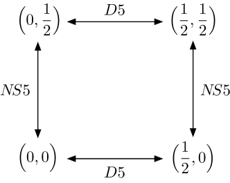
Figure 1: The effect of wrapped five-brane domain walls on discrete torsion.

The geometric arguments presented in this section apply to other isolated orbifold singularities besides $\mathbb{C}^{3}/\mathbb{Z}_{3}$, suggesting that in each case there should be three different gauge theories corresponding to the different choices of discrete torsion. Heuristically, since $n$ is odd the parent quiver theory has an odd number of nodes, and applying the rules outlined in appendix A of gauge will lead to (at least) one $SO$ or $U\!Sp$ gauge group factor. Thus, the pattern of discrete torsion can plausibly be explained in a manner closely analogous to the examples already discussed. Less trivially, we expect new gauge theory dualities relating the $SO$ and $U\!Sp$ theories. The appearance of these dualities is a highly nontrivial check on the discrete torsion classification presented above, and is the subject of the next section.

3 An infinite family of dual gauge theories

In this section we discuss the gauge theory dualities which arise from orientifolds of other $\mathcal{N}=1$ orbifold singularities. In particular, based on the arguments given in the previous section, we expect a dual pair of gauge theories and a self-dual gauge theory for every isolated orbifold singularity. As a nontrivial check of this conjecture, we write down the possible gauge theories for the orientifolds of an infinite family of orbifold singularities and show that two of three possibilities have matching anomalies, consistent with an S-duality relating these theories.

We focus our attention on the $z^{i}\to-z^{i}$ orientifolds of the orbifolds $\mathbb{C}^{3}/\mathbb{Z}_{n=2k+1}$ with the $\mathbb{Z}_{n}$ action

$$z^{1,2}\rightarrow\omega_{n}z^{1,2}\;\;,\;\;z^{3}\rightarrow\omega_{n}^{-2}z^{3}\,,$$ (22)

where $\omega_{n}\equiv\exp(2\pi i/n)$. The resulting geometry is toric, where the $U(1)^{3}$ toric isometry group is enhanced to $SU(2)\times U(1)\times U(1)_{R}$ with $SU(2)$ acting on the doublet $(z^{1},z^{2})$, except that in the special case of $\mathbb{C}^{3}/\mathbb{Z}_{3}$ (studied in gauge ) the isometry group is further enhanced to $SU(3)\times U(1)_{R}$ with $SU(3)$ acting on the triplet $(z^{1},z^{2},z^{3})$.

The toric diagram corresponding to this singularity is shown in figure 2(a).

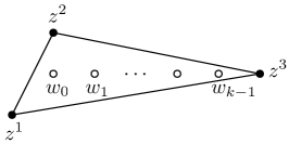
(a) Toric diagram with points labeled.

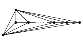
(b) Triangulated toric diagram.

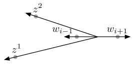
(c) Fan for the exceptional divisor $w_{i}=0$.

Figure 2: 2(a) The toric diagram for the $\mathbb{C}^{3}/\mathbb{Z}_{2k+1}$ orbifold discussed in the text. The black vertices $z^{1},z^{2},z^{3}$ are fields in the corresponding gauged linear sigma model (GLSM) (see e.g. Cox:1993fz ; Kennaway:2007tq ), whereas each internal point corresponds to an exceptional divisor. 2(b) Triangulating the toric diagram corresponds to fully resolving the geometry, where each internal point $w_{j}$ is now a GLSM field. 2(c) The fan for the exceptional divisor $w_{j}=0$, with a ray for each edge connected to $w_{j}$ in the triangulated toric diagram. For $j>0$, this is the fan for the Hirzebruch surface $\mathbb{F}_{2j+1}$, whereas for $j=0$ the left-facing ray is absent, and we obtain the fan for $\mathbb{P}^{2}$.

Fully resolving the singularity corresponds to triangulating the toric diagram, as in figure 2(b), giving a GLSM description with fields $z^{i}$ and $w_{j}$, $0\leq j<k$. Acting on the resolved geometry, one can show that the involution $z^{i}\to-z^{i}$ has fixed planes $w_{j}=0$ for $k-j$ odd, as well as a separate fixed point $z^{1}=z^{2}=w_{0}=0$ for even $k$. Thus, for odd $k$ there are $\frac{k+1}{2}$ $O7$ planes wrapping exceptional divisors $\mathbb{P}^{2}$ and $\mathbb{F}_{2j+1}$ for $0<j<k$ even (see figure 2(c)) where $\mathbb{F}_{m}$ denotes the $m$th Hirzebruch surface, whereas for even $k$ there are $k/2$ $O7$ planes wrapping exceptional divisors $\mathbb{F}_{2j+1}$ for $0<j<k$ odd as well as an $O3$ plane at a point on the $\mathbb{P}^{2}$.

To obtain the worldvolume gauge theory of $D3$ branes probing these orientifolds, we work within the framework of dimer models Hanany:2005ve ; Franco:2005rj . We refer the reader to Franco:2007ii for the state of the art on orientifolds of generic dimer models, and Franco:2010jv for a treatment in a dimer model language of a family of orientifolds similar to the one considered here and in strings-all . Brane/orientifold systems very similar to some of the ones we consider here have appeared in the literature many times before, most often studied in the CFT language. See for example Bianchi:1991eu ; Gimon:1996rq ; Berkooz:1996iz ; Angelantonj:1996uy ; Aldazabal:1997wi ; Antoniadis:1998ep ; Camara:2007dy ; Bianchi:2009bg for some relevant work on orientifolds and in particular orientifolds of orbifolds.

3.1 An infinite family S-dual gauge theories

In this subsection we derive the worldvolume gauge theories for $D3$ branes probing the infinite family of orientifold singularities considered above. As anticipated in §2, for each singularity we obtain three different gauge theories, two of which are expected to be S-dual. We demonstrate that the prospective S-dual gauge theories have matching anomalies. Other orbifold singularities not belonging to this infinite family are briefly considered in §3.2.

The brane tiling corresponding to the $\mathbb{C}^{3}/\mathbb{Z}_{n}$ orbifold singularity described above is shown in figure 3.

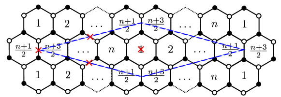
Figure 3: The brane tiling for the $\mathbb{C}^{3}/\mathbb{Z}_{n}$ orbifold singularity described in the text. The red crosses indicate the orientifold fixed points and the dashed blue line outlines the unit cell.

The tiling is invariant under reflection about a horizontal line through the middle row, which gives rise to a global $SU(2)$ symmetry in the corresponding gauge theory.

We focus on involutions of the dimer with isolated fixed points, since only these involutions can leave the global symmetries completely unbroken strings-all . Since there are $2n$ nodes in the unit cell and $n=2k+1$ is odd, the sign rule in Franco:2007ii requires the product of the four signs associated to the four orientifold fixed points to be odd. Due to the reflection symmetry there are six inequivalent choices. Labelling the fixed point signs counter-clockwise from the leftmost fixed point in figure 3, these are $(\mp,\pm,\pm,\pm)$, $(\pm,\mp,\pm,\pm)$, and $(\pm,\pm,\mp,\pm)$. Following the meson sign rules given in Franco:2007ii , we find the corresponding geometric involutions $z^{3}\to-z^{3}$, $z^{1}\to-z^{1}$ and $z^{i}\to-z^{i}$, respectively. Thus, the cases $(\mp,\pm,\pm,\pm)$, $(\pm,\mp,\pm,\pm)$ correspond to non-compact $O7$ planes, and lead to field theories with gauge anomalies in the absence of flavor branes.

The remaining two cases $(\pm,\pm,\mp,\pm)$ correspond to the desired $z^{i}\to-z^{i}$ involution, and lead to anomaly-free gauge theories for certain choices of the gauge group ranks. For $(-,-,+,-)$, we obtain the gauge group $\prod_{a=1}^{k}SU(N_{a})\times SO(N_{k+1})$ with the ranks fixed by anomaly cancellation to be $N_{a}=N-4\lfloor\tfrac{a}{2}\rfloor$ for some $N$. The charge table for this theory is

	$SU(N_{1})$	$SU(N_{2})$	$SU(N_{3})$	…	$SU(N_{k-1})$	$SU(N_{k})$	$SO(N_{k+1})$	$SU(2)$
$X^{i}$	$\overline{\ydiagram{1,1}}$	1	1	…	1	1	1	$\ydiagram{1}$
$Y$	$\ydiagram{1}$	$\ydiagram{1}$	1	…	1	1	1	1
$A^{i}_{(1)}$	$\ydiagram{1}$	$\overline{\ydiagram{1}}$	1	…	1	1	1	$\ydiagram{1}$
$B_{(1)}$	$\overline{\ydiagram{1}}$	1	$\ydiagram{1}$	…	1	1	1	1
$A^{i}_{(2)}$	1	$\ydiagram{1}$	$\overline{\ydiagram{1}}$	…	1	1	1	$\ydiagram{1}$
⋮	⋮	⋮	⋮	⋮	⋮	⋮	⋮	⋮
$A^{i}_{(k-1)}$	1	1	1	…	$\ydiagram{1}$	$\overline{\ydiagram{1}}$	1	$\ydiagram{1}$
$B_{(k-1)}$	1	1	1	…	$\overline{\ydiagram{1}}$	1	$\ydiagram{1}$	1
$A^{i}_{(k)}$	1	1	1	…	1	$\ydiagram{1}$	$\ydiagram{1}$	$\ydiagram{1}$
$Z$	1	1	1	…	1	$\overline{\ydiagram{1,1}}$	1	1

where we have omitted the abelian global symmetries, which are discussed below.

The remaining choice $(+,+,-,+)$ is related to the $SO$ theory described above by the negative rank duality discussed in appendix B of gauge . Therefore this theory has gauge group $\prod_{a=1}^{k}SU(\tilde{N}_{a})\times U\!Sp(\tilde{N}_{k+1})$ with $\tilde{N}_{a}=\tilde{N}+4\lfloor\tfrac{a}{2}\rfloor$ and charge table

	$SU(\tilde{N}_{1})$	$SU(\tilde{N}_{2})$	$SU(\tilde{N}_{3})$	…	$SU(\tilde{N}_{k-1})$	$SU(\tilde{N}_{k})$	$U\!Sp(\tilde{N}_{k+1})$	$SU(2)$
$\tilde{X}^{i}$	$\overline{\ydiagram{2}}$	1	1	…	1	1	1	$\ydiagram{1}$
$\tilde{Y}$	$\ydiagram{1}$	$\ydiagram{1}$	1	…	1	1	1	1
$\tilde{A}^{i}_{(1)}$	$\ydiagram{1}$	$\overline{\ydiagram{1}}$	1	…	1	1	1	$\ydiagram{1}$
$\tilde{B}_{(1)}$	$\overline{\ydiagram{1}}$	1	$\ydiagram{1}$	…	1	1	1	1
$\tilde{A}^{i}_{(2)}$	1	$\ydiagram{1}$	$\overline{\ydiagram{1}}$	…	1	1	1	$\ydiagram{1}$
⋮	⋮	⋮	⋮	⋮	⋮	⋮	⋮	⋮
$\tilde{A}^{i}_{(k-1)}$	1	1	1	…	$\ydiagram{1}$	$\overline{\ydiagram{1}}$	1	$\ydiagram{1}$
$\tilde{B}_{(k-1)}$	1	1	1	…	$\overline{\ydiagram{1}}$	1	$\ydiagram{1}$	1
$\tilde{A}^{i}_{(k)}$	1	1	1	…	1	$\ydiagram{1}$	$\ydiagram{1}$	$\ydiagram{1}$
$\tilde{Z}$	1	1	1	…	1	$\overline{\ydiagram{2}}$	1	1

where we once more omit the abelian global symmetries.

The superpotential for the $SO$ theory is

$$W=\epsilon_{ij}\operatorname{Tr}\left(X^{i}A^{j}_{(1)}Y+\sum_{a=1}^{k-1}A^{i}_{(a)}A^{j}_{(a+1)}B_{(a)}+A^{i}_{(k)}A^{j}_{(k)}Z\right)\,,$$ (23)

and for the $U\!Sp$ theory one has similarly

$$\tilde{W}=\epsilon_{ij}\operatorname{Tr}\left(\tilde{X}^{i}\tilde{A}^{j}_{(1)}\tilde{Y}+\sum_{a=1}^{k-1}\tilde{A}^{i}_{(a)}\tilde{A}^{j}_{(a+1)}\tilde{B}_{(a)}+\tilde{A}^{i}_{(k)}\tilde{A}^{j}_{(k)}\tilde{Z}\right)\,.$$ (24)

The quiver diagrams for the two gauge theories are shown in figure 4.

Figure 4: The quivers for the two gauge theories arising from orientifolding $D3$-branes probing the $\mathbb{C}^{3}/\mathbb{Z}_{n=2k+1}$ singularity. There are $k$ $SU$ factors. The $X^{i}$ and $Z$ matter fields of the $SO$ theory transform as $\overline{\ydiagram{1,1}}$ while the matter fields $\tilde{X}^{i}$ and $\tilde{Z}$ of the $U\!Sp$ model transform as $\overline{\ydiagram{2}}$.

In addition to the continuous $SU(2)\times U(1)\times U(1)_{R}$ global symmetry group, there are sometimes additional discrete symmetries. In particular, an extra $\mathbb{Z}_{n}$ symmetry appears whenever $N$ or $\tilde{N}$ is a multiple of $n$, whereas an extra $\mathbb{Z}_{2}$ symmetry is present in the $SO$ theory for even $N$. The latter arises from a combination of the $\mathbb{Z}_{2}$ outer automorphism group of $SO(2m)$ with a discrete flavor symmetry. Thus, a duality (if it exists) must relate the $U\!Sp$ theory and the odd-$N$ $SO$ theory with $N-\tilde{N}$ an odd multiple of $n$.

The fields carry the following charges under the $U(1)\times U(1)_{R}\times\mathbb{Z}_{n}$ symmetries  

	$X^{i}$	$Y$	$A^{i}_{(a)}$, $a$ odd
$U(1)$	$1$	$-2+\frac{2(n-3)}{N-4}$	$1+\frac{(n-2a+1)(a-1)}{N-2(a-1)}-\frac{(n-2a-1)(a+1)}{N-2(a+1)}$
$U(1)_{R}$	$\frac{2}{3}-\frac{n\mp 1}{N}$	$\frac{2}{3}+\frac{n\mp 1}{2N}+\frac{(n-3)5+3\pm 3}{6(N-4)}$	$\frac{2}{3}+\frac{(n-2a+1)(4a-1)+3\mp 3}{6(N-2(a-1))}-\frac{(n-2a-1)(4a+1)+3\pm 3}{6(N-2(a+1))}$
$\mathbb{Z}_{n}$	$\omega_{nN}^{-2}$	$\omega_{nN}\cdot\omega_{n(N-4)}^{3}$	$\omega_{n(N-2(a-1))}^{2a-1}\cdot\left[\omega_{n(N-2(a+1))}^{-2a-1}\right]^{1-\delta_{a,k}}$

	$B_{(a)}$, $a$ odd	$A^{i}_{(a)}$, $a$ even
$U(1)$	$-2-\frac{(n-2a+1)(a-1)}{N-2(a-1)}+\frac{(n-2a-3)(a+1)}{N-2(a+1)}$	$1+\frac{2a}{N-2a}$
$U(1)_{R}$	$\frac{2}{3}-\frac{(n-2a+1)(4a-1)+3\mp 3}{6(N-2(a-1))}+\frac{(n-2a-3)(4a+7)+3\mp 3}{6(N-2(a+1))}$	$\frac{2}{3}+\frac{10a-3(n\mp 1)}{3(N-2a)}$
$\mathbb{Z}_{n}$	$\omega_{n(N-2(a-1))}^{1-2a}\cdot\left[\omega_{n(N-2(a+1))}^{2a+3}\right]^{1-\delta_{a,k-1}}$	$\omega_{n(N-2a)}^{2a-1}\cdot\left[\omega_{n(N-2a)}^{-2a-1}\right]^{1-\delta_{a,k}}$

	$B_{(a)}$, $a$ even	$Z$
$U(1)$	$-2-\frac{(n-2a+1)a}{N-2a}+\frac{(n-2a-3)(a+2)}{N-2(a+2)}$	$-2-\frac{2(n-2\pm 1)}{N-n+2\mp 1}$
$U(1)_{R}$	$\frac{2}{3}-\frac{(n-2a+1)(4a-3)+3\pm 3}{6(N-2a)}+\frac{(n-2a-3)(4a+5)+3\pm 3}{6(N-2(a+2))}$	$\frac{2}{3}-\frac{2(2n-1\mp 1)}{3(N-n+2\mp 1)}$
$\mathbb{Z}_{n}$	$\omega_{n(N-2a)}^{1-2a}\cdot\left[\omega_{n(N-2(a+2))}^{2a+3}\right]^{1-\delta_{a,k-1}}$	$\omega_{n(N-n+2\mp 1)}^{-2(n-2)}$

where $\omega_{m}\equiv e^{2\pi i/m}$ and the upper/lower sign is for $k=(n-1)/2$ even/odd. The $U(1)\times U(1)_{R}\times\mathbb{Z}_{n}$ charges for the $U\!Sp$ theory are obtained by replacing $N\rightarrow-\tilde{N}$, as dictated by the negative rank duality relating the two theories.

Calculating the global anomalies that are relevant for anomaly matching in dual theories Csaki:1997aw one finds that the $SU(2)^{2}\,\mathbb{Z}_{n}$ anomaly as well as the gravitational $\mathbb{Z}_{n}$ and $U(1)$ anomalies vanish and the other anomalies are given by

	$SO$ theory	$U\!Sp$ theory
$SU(2)^{3}$	$\frac{1}{2}N(N-n)$ mod 2	$\frac{1}{2}\tilde{N}(\tilde{N}+n)$ mod 2
$SU(2)^{2}\,U(1)$	$\frac{1}{2}nN(N-n)$	$\frac{1}{2}n\tilde{N}(\tilde{N}+n)$
$SU(2)^{2}\,U(1)_{R}$	$\frac{1}{6}(\pm 3-n(2+n^{2}+N(N-n)))$	$\frac{1}{6}(\pm 3-n(2+n^{2}+\tilde{N}(\tilde{N}+n)))$
$U(1)^{3}$	$-3nN(N-n)$	$-3n\tilde{N}(\tilde{N}+n)$
$U(1)^{2}\,U(1)_{R}$	$-n(n^{2}\mp n+N(N-n))$	$-n(n^{2}\mp n+\tilde{N}(\tilde{N}+n))$
$U(1)\,U(1)_{R}^{2}$	$-\frac{1}{3}(n\pm 3)n(n\mp 1)$	$-\frac{1}{3}(n\pm 3)n(n\mp 1)$
$U(1)_{R}^{3}$	$\begin{array}[]{c}\frac{1}{18}(9\pm 90-n(99+6n(n\mp 1)\\ -8N(N-n)))\end{array}$	$\begin{array}[]{c}\frac{1}{18}(9\pm 90-n(99+6n(n\mp 1)\\ -8\tilde{N}(\tilde{N}+n)))\end{array}$
$U(1)_{R}$	$-\frac{1}{2}\left(5n-1\mp 4\right)$	$-\frac{1}{2}\left(5n-1\mp 4\right)$

where again the upper/lower sign is for $k$ even/odd. We conclude that the two theories have matching anomalies for $\tilde{N}=N-n$. This is a highly non-trivial check of our previous assertion that these theories should be S-dual, and is in perfect agreement with the arguments given in §2.

As an aside we note that the two dual theories have the same number of chiral multiplets and vector multiplets. In particular for $\tilde{N}=N-n$ we find for the $U\!Sp$ theory

number of vector multiplets: $$\frac{1}{6}(3\mp 9+n(n^{2}+5+3N(N-n))$$ (25)

number of chiral multiplets: $$\frac{1}{2}\left(6\pm 3+n\left(n^{2}-10+3N(N-n)\right)\right)$$ (26)

which agrees with the $SO$ theory where as usual the upper/lower sign is for $k$ even/odd. There is no obvious reason for the dual theories to be related in this fashion, and indeed the relation does not persist for nonorbifold singularities gauge ; strings-all .

For completeness, we describe $a$-maximization for these theories. To find the superconformal R-charge we define a trial R-symmetry under which the fields carry the charge $q_{R}+b\,q_{U(1)}$, where $q_{R}$ and $q_{U(1)}$ are the charges given above. Since the gravitational anomaly for the $U(1)$ flavor symmetry vanishes, $a$-maximization Intriligator:2003jj reduces to maximization with respect to $b$ of the $U(1)_{R}^{3}$ anomaly for the trial R-symmetry. We find for the $SO$ theory

$$b=-\frac{n(n\mp 1)+\!N(N-n)-\sqrt{n^{2}(n\mp 1)^{2}+\!N(N-n)(n\mp 3)(n\mp 1)+\!N^{2}(N-n)^{2}}}{3N(N-n)}\,,$$ (27)

where again the upper/lower signs are for $k=(n-1)/2$ even/odd. For the $U\!Sp$ theory $b$ is given by replacing $N\rightarrow-\tilde{N}$. Note that the vanishing of the gravitational $U(1)$ anomaly implies that the $U(1)_{R}^{2}\,U(1)$ anomaly vanishes after $a$-maximization. Using the above formula, the central charge and other anomalies involving the R-symmetry can easily be obtained. The results are rather lengthy, so we refrain from spelling them out explicitly.

3.2 Generalization to other orbifolds

A general supersymmetric $\mathbb{C}^{3}/\mathbb{Z}_{n}$ orbifold with an isolated singularity takes the form

$$z^{j}\rightarrow e^{\frac{2\pi ia_{j}}{n}}z^{j}$$ (28)

where $\sum a_{i}=0\bmod n$ and $\gcd(a_{i},n)=1$, so that $(a_{1},a_{2},a_{3})=(1,\ell,-\ell-1)$ for $\gcd(\ell,n)=\gcd(\ell+1,n)=1$. The first nontrivial example not belonging to the infinite family discussed above is the $\mathbb{Z}_{7}$ orbifold $(1,2,4)$. Choosing the same $z^{i}\to-z^{i}$ involution one obtains the gauge theories found in Kakushadze:1998tr . The gauge groups are $SO(N+4)\times SU(N)^{3}$ and $U\!Sp({\tilde{N}}-4)\times SU({\tilde{N}})^{3}$, where the explicit charge table is given in Table III of Kakushadze:1998tr . Both theories have a global $U(1)^{2}\times U(1)_{R}$ symmetry, and their anomalies match for ${\tilde{N}}=N+1$, as expected based on our arguments in §2.

We leave it to the interested reader to work out the details of other $\mathbb{Z}_{n}$ orbifolds with isolated singularities, which are expected to behave similarly to the cases studied here. For simplicity, we omit discussion of non-isolated singularities — such as for $\mathbb{Z}_{n}$ orbifolds with even $n$, $\mathbb{Z}_{m}\times\mathbb{Z}_{n}$ orbifolds with $\gcd(m,n)>1$, and nonabelian orbifolds — and proceed to discuss a different physical viewpoint on the duality.

4 The large volume picture

While the arguments presented in §2 provide a clear link between the duality relating the $\mathbb{C}^{3}/\mathbb{Z}_{3}$ $SO$ and $U\!Sp$ gauge theories and ten-dimensional S-duality, the interpretation of the duality in terms of branes is initially less obvious. Whereas the $\mathcal{N}=4$ case involved $O3$ planes, which transform into each other under $SL(2,\mathbb{Z})$, the $\mathbb{C}^{3}/\mathbb{Z}_{3}$ orientifold we consider corresponds to an $O7$ plane wrapping the $\mathbb{P}^{2}$ exceptional divisor. Since $O7$ planes do not transform simply under $SL(2,\mathbb{Z})$ (in particular, the S-dual of an $O7$ plane is not an $O7$ plane), the $\mathcal{N}=4$ story requires substantial modification to correctly describe the “microscopics” of how the duality acts on the fractional branes. The primary goal of the following sections is to develop this story. Along the way, we will also provide an explanation for the rank relation ${\tilde{N}}=N-3$ in terms of $D3$ charge conservation.

In order to systematically study D-branes in type IIB string theory, it is convenient to work in the framework of the derived category of coherent sheaves (we refer the reader to workingMath ; Sharpe:1999qz ; Douglas:2000gi ; Sharpe:2003dr ; Aspinwall:2004jr for excellent reviews and some of the original works on this topic in the physics literature). For completeness we review certain parts of this description below, highlighting those aspects that will be most important in our analysis. Much of the following formalism is well understood in the absence of orientifolds, see for example Douglas:2000qw ; Cachazo:2001sg ; Wijnholt:2002qz ; Herzog:2003dj ; Aspinwall:2004vm ; Wijnholt:2005mp ; Hanany:2006nm for some early works. The action of orientifolds on the derived category of coherent sheaves has been discussed in Diaconescu:2006id ; we follow the formalism and notation in that paper, extending it to include non-trivial $B_{2}$ fields and auto-equivalences of the category.

4.1 Preliminaries on derived categories and orientifolds

In the language of the derived category, branes are described by a complex of sheaves $\mathfrak{E}$ in an ambient space $X$. We will be interested in branes wrapping a complex surface $\mathcal{S}$ in a Calabi-Yau manifold $X$, with embedding map $i:\mathcal{S}\hookrightarrow X$, and supporting a sheaf $\mathscr{E}$, possibly with some non-trivial integer shift in the grading. In other words, we do not need to deal with general complexes, but only objects of the form $\mathfrak{E}=i_{*}\mathscr{E}[k]$, with $\mathscr{E}$ an ordinary sheaf on $\mathcal{S}$ and $k$ the position of $\mathscr{E}$ in the complex.

The branes $\mathscr{E}$ corresponding to the fractional branes at the singularity can be constructed by (left) mutation of a basic set of projective objects $\mathsf{P}_{i}$ BondalHelixes ; Cachazo:2001sg ; Feng:2002kk ; Herzog:2003dj ; Aspinwall:2004vm . On a del Pezzo surface $\mathcal{S}$ the $\mathsf{P}_{i}$ objects can be easily constructed as line bundles on $\mathcal{S}$, and there are systematic algorithms for finding such a collection Hanany:2006nm . We will give various examples below. The left mutation of a brane $\mathscr{F}_{i}$ through $\mathscr{F}_{j}$, denoted $\mathsf{L}_{\mathscr{F}_{j}}(\mathscr{F}_{i})$, is defined as Aspinwall:2004vm :

$$\mathsf{L}_{\mathscr{F}_{j}}(\mathscr{F}_{i})=\operatorname{Cone}\bigl{(}\operatorname{Hom}(\mathscr{F}_{j},\mathscr{F}_{i})\otimes\mathscr{F}_{j}\to\mathscr{F}_{i}\bigr{)}[-1]\,.$$ (29)

We refer the reader to Aspinwall:2004jr for a review of the cone construction. If one is only interested in the Chern characters of the branes, then (29) simplifies to:

$$\operatorname{ch}(\mathsf{L}_{\mathscr{F}_{j}}(\mathscr{F}_{i}))=\operatorname{ch}(\mathscr{F}_{i})-\chi(\mathscr{F}_{j},\mathscr{F}_{i})\operatorname{ch}(\mathscr{F}_{j})\,,$$ (30)

with

$$\chi(\mathscr{F}_{j},\mathscr{F}_{i})=\int_{\mathcal{S}}\operatorname{ch}(\mathscr{F}_{j}^{\vee})\wedge\operatorname{ch}(\mathscr{F}_{i})\wedge\operatorname{Td}(T_{\mathcal{S}})\,.$$ (31)

Using these definitions, a basis of fractional branes can be constructed by taking:

$$\begin{split}\mathscr{E}_{1}&=\mathsf{P}_{1}\,,\\ \mathscr{E}_{2}&=\mathsf{L}_{\mathsf{P}_{1}}\mathsf{P}_{2}\,,\\ &\cdots\\ \mathscr{E}_{n-1}&=\mathsf{L}_{\mathsf{P}_{1}}\mathsf{L}_{\mathsf{P}_{2}}\cdots\mathsf{L}_{\mathsf{P}_{n-2}}\mathsf{P}_{n-1}\,,\\ \mathscr{E}_{n}&=\mathsf{L}_{\mathsf{P}_{1}}\mathsf{L}_{\mathsf{P}_{2}}\cdots\mathsf{L}_{\mathsf{P}_{n-1}}\mathsf{P}_{n}\,.\end{split}$$ (32)

Now that we know how to construct the fractional branes at the singularity in terms of geometric objects, we want to define a suitable orientifold action. Consider first the case with vanishing $B_{2}$ field. In the case that the orientifold wraps $\mathcal{S}$ itself, the action on the fractional branes is given by Diaconescu:2006id

$$i_{*}\mathscr{E}[k]\longrightarrow i_{*}(\mathscr{E}^{\vee}\otimes K_{\mathcal{S}})[2-k]\,,$$ (33)

with $K_{\mathcal{S}}$ the anti-canonical class of $\mathcal{S}$. This agrees with the usual large volume action on $D7$s, which is generally considered only at the level of Chern classes. In this case (33) maps $D7$s to $D7s$ and $\overline{D7}$s to $\overline{D7}$s. Furthermore, the worldvolume flux $F$ on the brane is related to $\mathscr{E}$ by $F=\mathscr{E}\otimes K_{\mathcal{S}}^{-1/2}$ Katz:2002gh . Acting on $F$, (33) then gives $F\to F^{\vee}$, in agreement with the usual prescription.

Incorporating a $B_{2}$ field in $H^{2}(\mathcal{S},\mathbb{R})$ is relatively straightforward. Usually one introduces a quantity $\mathcal{F}=c_{1}(\mathscr{F})-B_{2}$, with $c_{1}(\mathscr{F})$ the field strength for the connection in the bundle $\mathscr{F}$, in terms of which the orientifold acts as $\mathcal{F}\to-\mathcal{F}$.

However, there is an equivalent alternative viewpoint that fits better with the derived-category description of branes. Notice that since orientifolds map $B_{2}\to-B_{2}$, only half-integrally quantized $B_{2}$ fields are allowed, and we can view $2B_{2}$ as the field strength of a line bundle $\mathcal{L}_{2B_{2}}$. The orientifold therefore has a double effect: it acts on the D-branes as in (33) while also reflecting the real part of the Kähler moduli space. We can trivially undo the action on Kähler moduli space (so we can compare branes and their images at the same point in moduli space) by shifting $-B_{2}\to-B_{2}+2B_{2}=B_{2}$. Due to the invariance of the theory under joint integral shifts of $B_{2}$ and the bundles on the branes, this is equivalent to tensoring the sheaf $\mathscr{E}$ on the brane by $\mathcal{L}_{2B_{2}}$. Thus, in the presence of $B_{2}\in H^{2}(\mathcal{S},\mathbb{R})$, (33) gets amended to

$$i_{*}\mathscr{E}[k]\longrightarrow i_{*}(\mathscr{E}^{\vee}\otimes K_{\mathcal{S}}\otimes\mathcal{L}_{2B_{2}})[2-k]\,.$$ (34)

This action can also be understood purely in terms of the derived category, forgetting about the physical origin of $\mathcal{L}_{2B_{2}}$. From this viewpoint, (34) generalizes the ordinary action of the orientifold by twisting the elements of the category with a line bundle. Twisting all the elements of the category by the same line bundle is an autoequivalence of the category, so we have our first example of an orientifold that combines the ordinary large-volume orientifold action with an auto-equivalence of the derived category. We discuss a variation of this idea below, which turns out to be useful in understanding the orientifolds of various quiver configurations.

While the description of the branes in terms of the derived category of coherent sheaves is relatively simple (at least in comparison with the objects in the mirror description, the Fukaya category, see Aspinwall:2004jr for a review), there is an important complication: as we move in Kähler moduli space the supersymmetry preserved by the D-branes changes, in a way highly influenced by world-sheet instanton corrections. The most convenient way to deal with this issue is by considering the central charge $Z(\mathscr{E},t)$, with $\mathscr{E}$ our brane of interest and $t=B_{2}+iJ$ our position in complexified Kähler moduli space. At large volume, where we can ignore $\alpha^{\prime}$ corrections, a brane $\mathscr{E}$ wrapping $\mathcal{S}$ has central charge

$$Z(\mathscr{E}[k],t)=(-1)^{k}\int_{\mathcal{S}}e^{-t}\operatorname{ch}(\mathscr{E})\sqrt{\frac{\operatorname{Td}(T_{\mathcal{S}})}{\operatorname{Td}(N_{\mathcal{S}})}}\,.$$ (35)

It will be convenient to introduce a charge vector for the brane given by:

$$\Gamma(\mathscr{E}[k])=(-1)^{k}[S]\,\operatorname{ch}(\mathscr{E})\sqrt{\frac{\operatorname{Td}(T_{\mathcal{S}})}{\operatorname{Td}(N_{\mathcal{S}})}}$$ (36)

in terms of which the large volume central charge is given by:

$$Z(\mathscr{E}[k],t)=\int_{X}e^{-t}\,\Gamma(\mathscr{E}[k])\,.$$ (37)

One can incorporate $\alpha^{\prime}$ corrections to the central charge by going to the mirror of the configuration in question. In what follows, we quote the relevant results as needed, referring the interested reader to Cox:2000vi ; Hori:2003ic ; Aspinwall:2004jr for surveys of the techniques required to derive these results and further references.

Once we have the set of branes and the orientifold action we can compute the spectrum of light states. The precise calculation requires computation of $\operatorname{Ext}$ groups Katz:2002gh . In the particular case that we will be considering — $\operatorname{Ext}$ groups between sheaves $A$, $B$ supported on a surface $\mathcal{S}$ in the Calabi-Yau $X$ — there is a one-term spectral sequence SeidelThomas ; Katz:2002gh giving the $\operatorname{Ext}$ groups in $X$ in terms of $\operatorname{Ext}$ groups in $\mathcal{S}$:

$$\begin{split}\operatorname{Ext}^{k}_{X}(i_{*}A,i_{*}B)&=\sum_{p+q=k}\operatorname{Ext}^{p}_{\mathcal{S}}(A,B\wedge N_{\mathcal{S}}^{q})\\ &=\operatorname{Ext}^{k}_{\mathcal{S}}(A,B)\oplus\operatorname{Ext}^{k-1}_{\mathcal{S}}(A,B\otimes K_{\mathcal{S}})\,,\end{split}$$ (38)

where in the second line we have used the fact that $\mathcal{S}$ is a divisor in a Calabi-Yau, so $N_{\mathcal{S}}=K_{\mathcal{S}}$. Using Serre duality on $\mathcal{S}$ we can rewrite the final expression as:

$$\operatorname{Ext}^{k}_{X}(i_{*}A,i_{*}B)=\operatorname{Ext}_{\mathcal{S}}^{k}(A,B)\oplus\operatorname{Ext}_{\mathcal{S}}^{3-k}(B,A)^{\vee}\,.$$ (39)

If one were interested only in the dimensions of the $\operatorname{Ext}$ groups the dual sign in the second term could be ignored, but we will keep it as it nicely encodes some of the flavor structure of the quiver, as demonstrated in some of the examples below.

For our purposes it is usually sufficient to compute only the chiral index of states between the branes. This is defined as:

$$\bigl{\langle}\mathscr{E}_{i},\mathscr{E}_{j}\bigr{\rangle}=\sum(-1)^{k}\operatorname{Ext}^{k}_{X}(\mathscr{E}_{i},\mathscr{E}_{j})\,,$$ (40)

with $X$ the Calabi-Yau threefold. As is often the case with an index, this expression can be expressed as an integral of forms on $X$. In particular, it is given by the Dirac-Schwinger-Zwanziger (DSZ) product of the corresponding charge vectors:

$$\bigl{\langle}\mathscr{E}_{i},\mathscr{E}_{j}\bigr{\rangle}=\sum_{k}(-1)^{k}\int_{X}\Gamma^{(2k)}(\mathscr{E}_{i})\,\,\wedge\,\,\Gamma^{(6-2k)}(\mathscr{E}_{j})\,,$$ (41)

with $\Gamma^{(m)}$ denoting the part of $\Gamma$ of degree m. This product is clearly antisymmetric, and in fact it is the mirror to the usual intersection product in IIA. Since we have branes wrapping a complex surface $\mathcal{S}$, the charge vector takes the form:

$$\Gamma(\mathscr{E}_{i})=[\mathcal{S}]\wedge\left(\omega^{(i)}_{0}+\omega^{(i)}_{2}+\omega^{(i)}_{4}\right)\,,$$ (42)

with $\omega_{n}\in H^{n}(\mathcal{S},\mathbb{R})$. Eq. (41) then simplifies to:

$$\bigl{\langle}\mathscr{E}_{i},\mathscr{E}_{j}\bigr{\rangle}=\int_{\mathcal{S}}c_{1}(T_{\mathcal{S}})\wedge\left(\omega_{0}^{(i)}\wedge\omega_{2}^{(j)}-\omega_{0}^{(j)}\wedge\omega_{2}^{(i)}\right)\,,$$ (43)

where we have used adjunction: $c_{1}([\mathcal{S}]|_{\mathcal{S}})=c_{1}(N_{\mathcal{S}})=-c_{1}(T_{\mathcal{S}})$, since $X$ is a Calabi-Yau manifold.

Number of chiral multiplets	Representation
$\bigl{\langle}\mathscr{E}_{i},\mathscr{E}_{j}\bigr{\rangle}$	$(\ydiagram{1}_{i},\overline{\ydiagram}{1}_{j})$
$\bigl{\langle}\mathscr{E}_{i},\mathscr{E}_{j}^{\prime}\bigr{\rangle}$	$(\ydiagram{1}_{i},\ydiagram{1}_{j})$
$\frac{1}{2}\bigl{\langle}\mathscr{E}_{i},\mathscr{E}_{i}^{\prime}\bigr{\rangle}+\frac{1}{8}\bigl{\langle}e^{-B_{2}}\mathscr{E}_{i},O7^{\pm}\bigr{\rangle}$	$\ydiagram{2}_{\,i}$
$\frac{1}{2}\bigl{\langle}\mathscr{E}_{i},\mathscr{E}_{i}^{\prime}\bigr{\rangle}-\frac{1}{8}\bigl{\langle}e^{-B_{2}}\mathscr{E}_{i},O7^{\pm}\bigr{\rangle}$	$\ydiagram{1,1}_{\,i}$

Table 1: Spectrum of chiral multiplets charged under brane $\mathscr{E}_{i}$ in the presence of a $O7^{\pm}$ plane. $\mathscr{E}_{j}$ denotes a generic brane intersecting $\mathscr{E}_{i}$, and primes denote image branes. Any resulting negative signs should be interpreted as conjugate representations. Notice that $\mathscr{E}_{i}$ refers to the basic fractional branes, we count multiplicities separately.

Orientifold planes will also contribute to the D-brane charges. The charge vector for an $O7$ plane is given by:

$$\Gamma(O7^{\pm})=\pm 8[\mathcal{S}]\wedge\sqrt{\frac{\hat{L}(T_{\mathcal{S}}/4)}{\hat{L}(N_{\mathcal{S}}/4)}}=\pm[\mathcal{S}]\wedge\left(8-\frac{1}{6}c_{2}(T_{\mathcal{S}})\right)\,,$$ (44)

with $\hat{L}$ the Hirzebruch genus $\hat{L}(E)=1+\frac{1}{3}(c_{1}^{2}(E)-2c_{2}(E))+\ldots$, where we have omitted terms of degree 6 or higher, since they vanish on $\mathcal{S}$. In the presence of such an orientifold, the spectrum gets truncated to invariant states, given by bifundamentals and (anti-)symmetric representations. The precise matter content in the presence of the orientifold plane can be read off from the mirror formulas in IIA Blumenhagen:2000wh ; Ibanez:2001nd ; Cvetic:2001tj ; Cvetic:2001nr ; Marchesano:2007de . Given branes $\mathscr{E}_{i},\mathscr{E}_{j}$ with orientifold images $\mathscr{E}_{i}^{\prime},\mathscr{E}_{j}^{\prime}$ respectively, one obtains the spectrum in table 1.

As in Cvetic:2001nr , this spectrum can essentially be derived from tadpole/anomaly cancellation and linearity of the DSZ product. Tadpole cancellation requires that the 4-form and 2-form parts of the charge vectors satisfy:

$$\Gamma(O7^{\pm})+\sum e^{-B_{2}}\Gamma(\mathscr{E}_{i})=0\,,$$ (45)

where the sum is over all branes in our configuration, including images under the orientifold involution and multiplicities for non-abelian stacks. We have added the $B_{2}$ field explicitly, since we did not include it in our definition of the charge vector (36), but it enters in the definition of the Chern-Simons charge. Consider now a fractional brane $\mathscr{E}_{i}$ not invariant under the orientifold involution, and let us put a stack of $N_{i}(\mathscr{E}_{i}+\mathscr{E}_{i}^{\prime})$ branes on our singularity, with gauge group $U(N_{i})$. Taking the DSZ product of (45) with $e^{-B_{2}}\Gamma(\mathscr{E}_{i})$ one gets (with a slight abuse of notation):

$$\sum_{j\neq i,i^{\prime}}\bigl{\langle}\mathscr{E}_{i},\mathscr{E}_{j}\bigr{\rangle}+\bigl{\langle}\mathscr{E}_{i},N_{i}\mathscr{E}_{i}^{\prime}\bigr{\rangle}+\bigl{\langle}e^{-B_{2}}\mathscr{E}_{i},O7^{\pm}\bigr{\rangle}=0\,,$$ (46)

where we have used the fact that the DSZ product is an index, so it does not change by deforming both sides by the same $B_{2}$ field, and in particular the $B_{2}$ field can be ignored if it appears in both sides of the DSZ product. (The 6-form part of the charges (i.e. the $D3$ charge) was not constrained by (45), but since we have no Calabi-Yau filling branes in our background the $D9$-$D3$ contribution drops out of (46) anyway.) Notice that the first term in (46) is just the field theory anomaly coming from the chiral fields in the fundamental representation of $U(N_{i})$, in conventions where each chiral fundamental field contributes 1 unit to the anomaly. The second and third terms must then equal the net anomaly coming from two-index tensors:

$$n_{\scalebox{0.7}{$\ydiagram{2}$}}(N_{i}+4)+n_{\scalebox{0.7}{$\ydiagram{1,1}$}}(N_{i}-4)=N_{i}\bigl{\langle}\mathscr{E}_{i},\mathscr{E}_{i}^{\prime}\bigr{\rangle}+\bigl{\langle}e^{-B_{2}}\mathscr{E}_{i},O7\bigr{\rangle}\,.$$ (47)

Imposing that the relation is satisfied for any $N_{i}$ we obtain the relations in table 1.

Finally, given a generic brane $\mathscr{E}_{i}$, one has $\operatorname{Ext}^{0}(\mathscr{E}_{i},\mathscr{E}_{i})$ gauge bosons from the brane to itself. In the absence of orientifolds, this gives rise to a $U(N_{i})$ gauge stack, with $N_{i}^{2}=\dim\operatorname{Ext}^{0}(\mathscr{E}_{i},\mathscr{E}_{i})$. If the brane is invariant under the orientifold projection, the involution projects $U(N_{i})$ to either $U\!Sp(N_{i})$ or $SO(N_{i})$. If the brane is not invariant, but is mapped to an image brane instead, then the original $U(N_{i})\times U(N_{i})$ gauge group gets projected down to $U(N_{i})$.

4.2 Large volume description of the orientifolded $\mathbb{C}^{3}/\mathbb{Z}_{3}$ quiver

Let us put what we just described into practice. The theory for branes at a $\mathbb{C}^{3}/\mathbb{Z}_{3}$ is conventionally described by the exceptional collection

$$\mathcal{C}=\{\mathcal{O}[0],\Omega(1)[1],\mathcal{O}(-1)[2]\}$$ (48)

with $\Omega$ the cotangent bundle on $\mathbb{P}^{2}$. This collection can be obtained by mutation of the basic set of projective objects:

$$\mathsf{P}=\{\mathcal{O},\mathcal{O}(1),\mathcal{O}(2)\}\,.$$ (49)

In our case it will be convenient to tensor all the elements in the collection with $\mathcal{O}(-1)$, and thus we will be dealing with the following collection instead:

$$\mathcal{C}=\{\mathcal{O}(-1)[0],\Omega[1],\mathcal{O}(-2)[2]\}\,.$$ (50)

The reason for tensoring with $\mathcal{O}(-1)$ is simple: since we want to orientifold, the branes that we identify under the involution should have the same mass, but it is not hard to see using the explicit expressions for the central charge given below that the elements of (48) have different central charges, and thus different masses. Tensoring the whole basis by a line bundle does not change the quiver structure, but it changes the central charge and hence fixes the problem. To wit, if we have a $D7$ brane wrapping $\mathcal{S}$ with charge vector

$$\Gamma(D7)=[\mathcal{S}]\wedge(Q_{0}+Q_{2}\ell+Q_{4}\ell^{2})$$ (51)

with $\ell$ the hyperplane in $\mathcal{S}=\mathbb{P}^{2}$, then its exact central charge is given by Aspinwall:2004jr

$$Z(D7)=\left(\frac{Q_{0}}{2}-Q_{2}\right)\Phi_{1}+\left(\frac{1}{2}Q_{0}\right)\Phi_{2}+\frac{1}{12}Q_{0}+Q_{4}\,,$$ (52)

where $\Phi_{i}$ are the quantum periods. We will discuss these periods in more detail in section 6, but for our current purposes we will only need the fact that they vanish at the quiver point, where

$$Z^{\bullet}(D7)=\frac{1}{12}Q_{0}+Q_{4}\,.$$ (53)

This implies in particular that:

$$\begin{split}Z^{\bullet}(\mathcal{O}(n))&=\frac{1}{12}+\left(\frac{1}{2}n^{2}+\frac{3}{2}n+\frac{5}{4}\right)\\ Z^{\bullet}(\mathcal{O}(n-1))&=\frac{1}{12}+\left(\frac{1}{2}n^{2}+\frac{1}{2}n+\frac{1}{4}\right)\,.\end{split}$$ (54)

Imposing that both central charges are equal gives $n=-1$, as claimed. Tensoring the collection by $\mathcal{O}(-1)$ can also be achieved by a change in conventions, see Aspinwall:2004jr for an example.

The charge vectors for the fractional branes in (50) are given by:

$$\begin{split}\Gamma(\mathcal{O}(-1)[0])=[\mathcal{S}]\wedge\operatorname{ch}(\mathcal{O}(-1))\sqrt{\frac{\operatorname{Td}(T_{\mathcal{S}})}{\operatorname{Td}(N_{\mathcal{S}})}}&=[\mathcal{S}]\wedge\left(1+\frac{1}{2}\ell+\frac{1}{4}\ell^{2}\right)\\ \Gamma(\Omega[1])=-[\mathcal{S}]\wedge\operatorname{ch}(\Omega)\sqrt{\frac{\operatorname{Td}(T_{\mathcal{S}})}{\operatorname{Td}(N_{\mathcal{S}})}}&=[\mathcal{S}]\wedge\left(-2+\frac{1}{2}\ell^{2}\right)\\ \Gamma(\mathcal{O}(-2)[2])=[\mathcal{S}]\wedge\operatorname{ch}(\mathcal{O}(-2))\sqrt{\frac{\operatorname{Td}(T_{\mathcal{S}})}{\operatorname{Td}(N_{\mathcal{S}})}}&=[\mathcal{S}]\wedge\left(1-\frac{1}{2}\ell+\frac{1}{4}\ell^{2}\right)\,.\end{split}$$ (55)

Plugging these expressions in (53) we easily see that

$$Z^{\bullet}(\mathcal{O}(-1)[-1])=Z^{\bullet}(\Omega[0])=Z^{\bullet}(\mathcal{O}(-2)[1])=\frac{1}{3}\,,$$ (56)

which is what one expects from the $\mathbb{Z}_{3}$ symmetry permuting the fractional branes. For illustration we show the behavior of the central charges as we go to large volume in figure 5, where we have used the explicit form (98) of the periods $\Phi_{i}$ and the mirror map Cox:2000vi , which in our case is just $B_{2}+iJ=\Phi_{1}(z)$.

Figure 5: Phase of the central charges for the $\mathbb{C}^{3}/\mathbb{Z}_{3}$ fractional branes as we go from the quiver point at $J=B_{2}=0$ towards large volume ($J=+\infty$) along the $B_{2}=0$ line. The central charge of $\Omega[1]$ stays real and positive, so we do not show it. The phases of $\mathcal{O}(-2)[2]$ and $\mathcal{O}(-1)[0]$ asymptote to $\pm\pi$.

Using (33) it is straightforward to check that (50) maps to itself under the orientifold involution. In the case of the line bundles this is easy to see:

$$i_{*}\mathcal{O}(-1)[0]\longrightarrow i_{*}(\mathcal{O}(-1)^{\vee}\wedge K_{\mathcal{S}})[2]=i_{*}(\mathcal{O}(1)\wedge\mathcal{O}(-3))[2]=i_{*}\mathcal{O}(-2)[2]\,.$$ (57)

The case of $\Omega[1]$ is slightly more complicated, but follows from the fact that $\Omega^{\vee}\otimes K_{\mathcal{S}}=\Omega$, so the brane maps to itself:

$$i_{*}\Omega[1]\longrightarrow i_{*}(\Omega^{\vee}\otimes K_{\mathcal{S}})[2-1]=i_{*}\Omega[1]\,.$$ (58)

We can in fact derive the quiver in full detail. By (55), we know that $\Omega[1]$ has $D7$ charge equal to $-2$, so we can cancel the $D7$ brane tadpole by adding 4 $\Omega[1]$ branes. Since $\Omega[1]$ maps to itself, and it has $\dim\operatorname{Ext}^{0}(\Omega[1],\Omega[1])=1$, we see that under the $O7^{+}$ action the resulting stack is $U\!Sp(4)$. We can add $k$ pairs of regular $D3$ branes, and thus enhance the symmetry to $U\!Sp(2k+4)\times U(2k)$. The intersection products are easily computed using (55), (43) and the fact that $c_{1}(T_{\mathcal{S}})=c_{1}(\mathcal{O}(3))=3\ell$:

$$\begin{split}\bigl{\langle}\Omega[1],\mathcal{O}(-1)[0]\bigr{\rangle}&=\int_{\mathbb{P}^{2}}(3\ell)\wedge\left(-2\cdot\frac{1}{2}\ell\right)=-3\\ \bigl{\langle}\mathcal{O}(-1)[0],\mathcal{O}(-2)[2]\bigr{\rangle}&=-3\\ \bigl{\langle}\mathcal{O}(-1)[0],O7^{+}\bigr{\rangle}&=-12\,.\end{split}$$ (59)

By applying the rules in table 1 we thus find the following matter content:

$$\begin{array}[]{cc|c}U\!Sp(2k+4)&U(2k)&SU(3)\\ \hline\cr\overline{\ydiagram}{1}&\ydiagram{1}&\ydiagram{1}\\ 1&\overline{\ydiagram}{2}&\ydiagram{1}\end{array}$$ (63)

with the $SU(3)$ being a global symmetry, which at this level simply encodes the multiplicity of the matter fields. We will see in some simpler examples below how this group of global symmetries can also be understood geometrically, but we avoid the discussion of this particular case since it is slightly more technical.

Central charge for the orientifold.

Let us assume that the mass of the orientifold can be computed exactly (including all $\alpha^{\prime}$ corrections) in a manner similar to that of a $D7$ brane. We will analyze the $O7^{+}$ plane, and assume that it has the same argument for the central charge as the $O7^{-}$ plane (i.e. they preserve the same supersymmetries). Using the same notation as above, we have from (44) that $Q_{0}=8$, $Q_{2}=0$, $Q_{4}=-\chi(\mathbb{P}^{2})/6=-\frac{1}{2}$. The central charge at the quiver point is thus:

$$Z^{\bullet}(O7^{+})=\frac{8}{12}-\frac{1}{2}=\frac{1}{6}>0\,.$$ (64)

The central charge at large volume, on the other hand, is given by:

$$\begin{split}Z^{lv}(O7^{+})&=8\int_{S}e^{-B_{2}-iJ}\sqrt{\frac{\hat{L}(TS/4)}{\hat{L}(NS/4)}}\\ &\xrightarrow{vol(S)\to\infty}-8\int_{S}J^{2}<0\,.\end{split}$$ (65)

As it is clear, the central charge of the orientifold changes sign in going from large to small volume, and in particular, since it is a real quantity, it passes through 0 (the vanishing point is located at $J\approx 0.0694$). Close to the quiver point, the orientifold has a phase of the central charge opposite to the one at large volume. So we learn that the supersymmetry preserved by the $O7^{\pm}$ orientifold at the quiver point is opposite to the one preserved at large volume, and furthermore it is the same supersymmetry preserved by the fractional branes (50).

4.3 Quantum symmetries and ærientifolds

As we have just seen, the orientifold action (33) left the fractional brane $\Omega[1]$ invariant, while it exchanged $\mathcal{O}(-1)[0]$ and $\mathcal{O}(-2)[2]$. This beautifully reproduces the quiver structure obtained via CFT or orientifolded dimer model techniques. However, a longer look to the quiver may leave one puzzled: from the point of view of the quiver gauge theory there is nothing special about the node associated with the $\Omega[1]$ brane, one could have taken an involution of the quiver leaving invariant any of the other two nodes. This is in fact true in the full string theoretic description, and in the present language follows from the fact that the derived category has auto-equivalences, as we now explore.

We will not go into details of the mathematical meaning of auto-equivalences (we refer the reader to Aspinwall:2004jr for a detailed review), but we can think of an auto-equivalence of the derived category as a re-labeling of the D-branes in such a way that the physics is unaffected. We have already encountered a simple auto-equivalence of the derived category in section 4.1, where we discussed integer shifts of the $B_{2}$ field. Another familiar context in which this phenomenon arises is that of monodromy around a conifold point. Consider for example a point in moduli space where a brane $\mathscr{F}$ becomes massless. As we circle once around this point in moduli space the charges of the branes shift as Candelas:1990rm ; Hori:2000ck :

$$\Gamma(\mathscr{E})\to\Gamma(\mathscr{E})-\bigl{\langle}\mathscr{E},\mathscr{F}\bigr{\rangle}\Gamma(\mathscr{F})\,.$$ (66)

As we see, the charges of most branes will change, but this cannot induce a change in the physics of the background or the set of stable branes, since we end up at the same point in moduli space. The operation must then amount to a relabeling of the D-brane charges.

In our particular context the conifold points in moduli space are precisely those where the fractional branes in the quiver point become massless. In particular, we will present the moduli space in such a way that it is $\mathcal{O}(-1)[0]$ that becomes massless. The induced action on the charge vectors as we go around the point where $\mathcal{O}(-1)[0]$ becomes massless is:

$$\Gamma(\mathscr{E})\to\Gamma(\mathscr{E})-\bigl{\langle}\mathscr{E},\mathcal{O}(-1)\bigr{\rangle}\Gamma(\mathcal{O}(-1))\,.$$ (67)

Since this is a linear transformation, it is convenient to rewrite this as a matrix action on the charge vector:

$$\begin{pmatrix}\Gamma^{(2)}\\ \Gamma^{(4)}\\ \Gamma^{(6)}\end{pmatrix}\to\begin{pmatrix}-\frac{1}{2}&3&0\\ -\frac{3}{4}&\frac{5}{2}&0\\ -\frac{3}{8}&\frac{3}{4}&1\end{pmatrix}\begin{pmatrix}\Gamma^{(2)}\\ \Gamma^{(4)}\\ \Gamma^{(6)}\end{pmatrix}\equiv\mathcal{M}_{C}\begin{pmatrix}\Gamma^{(2)}\\ \Gamma^{(4)}\\ \Gamma^{(6)}\end{pmatrix}$$ (68)

where as usual $\Gamma^{(2i)}$ denotes the $2i$-form part of $\Gamma$.

A similar phenomenon that appears in our context is monodromy around the large volume point, which shifts the $B_{2}$ field by one unit, or equivalently it acts on the charges as:

$$\Gamma(\mathscr{E})\to\Gamma(\mathscr{E})\wedge\operatorname{ch}(\mathcal{O}(-1))\,.$$ (69)

Again writing this monodromy in matrix form, we have:

$$\begin{pmatrix}\Gamma^{(2)}\\ \Gamma^{(4)}\\ \Gamma^{(6)}\end{pmatrix}\to\begin{pmatrix}1&0&0\\ -1&1&0\\ \frac{1}{2}&-1&1\end{pmatrix}\begin{pmatrix}\Gamma^{(2)}\\ \Gamma^{(4)}\\ \Gamma^{(6)}\end{pmatrix}\equiv\mathcal{M}_{LV}\begin{pmatrix}\Gamma^{(2)}\\ \Gamma^{(4)}\\ \Gamma^{(6)}\end{pmatrix}\,.$$ (70)

The moduli space of $\mathbb{C}_{3}/\mathbb{Z}_{3}$ is a $\mathbb{P}^{1}$ with three marked points around which monodromy occurs: the large volume point, the conifold point, and the quiver point. The total monodromy around all three points must then vanish, and in this way we can easily obtain the monodromy around the quiver point:

$$\mathcal{M}_{Q}=\bigl{(}\mathcal{M}_{LV}\mathcal{M}_{C}\bigr{)}^{-1}=\begin{pmatrix}-\frac{1}{2}&-3&0\\ \frac{1}{4}&-\frac{1}{2}&0\\ \frac{1}{8}&\frac{1}{4}&1\end{pmatrix}\,.$$ (71)

It is straightforward to show that $\mathcal{M}_{Q}^{3}=1$, and furthermore, from the charges (55):

$$\begin{split}\mathcal{M}_{Q}\Gamma(\mathcal{O}(-1)[0])&=\Gamma(\Omega[1])\,,\\ \mathcal{M}_{Q}\Gamma(\Omega[1])&=\Gamma(\mathcal{O}(-2)[2])\,,\\ \mathcal{M}_{Q}\Gamma(\mathcal{O}(-2)[2])&=\Gamma(\mathcal{O}(-1)[0])\,.\end{split}$$ (72)

We therefore identify $\mathcal{M}_{Q}$ with the quantum symmetry rotating the quiver.

We are now in a position to resolve the issue that we presented at the beginning of this section. Denoting the ordinary orientifold involution (33) by $\mathcal{P}$ (which acts on the charges as $\operatorname{diag}(1,-1,1)$), one can construct a new class of orientifolds by composing with the auto-equivalences of the category just described. We call the resulting object an ærientifold, in order to distinguish it from the ordinary large volume orientifold given by $\mathcal{P}$, although we emphasize that ærientifolds are just as natural from the quiver point of view. For example, the ærientifold leaving the $\mathcal{O}(-1)[0]$ node invariant would be defined by $\mathcal{P}^{\prime}=\mathcal{M}_{Q}^{-1}\mathcal{P}\mathcal{M}_{Q}$, and the one leaving $\mathcal{O}(-2)[2]$ invariant would be $\mathcal{P}^{\prime\prime}=\mathcal{M}_{Q}\mathcal{P}\mathcal{M}_{Q}^{-1}$. At the level of charges we have that:

$$\mathcal{P}^{\prime}=\begin{pmatrix}-\frac{1}{2}&3&0\\ \frac{1}{4}&\frac{1}{2}&0\\ \frac{1}{8}&-\frac{1}{4}&1\end{pmatrix}\,.$$ (73)

We see that from the quiver point of view it is very natural to dress the ordinary large volume action of the orientifold with auto-equivalences of the category, and such dressings appear very naturally when orbifolding the quiver for certain singularities.

4.4 Microscopic description of the discrete torsion

We now connect the classification of the different orientifolds based on discrete torsion advocated in section 2 with the large volume picture discussed in this section. To do so, we make use of the fact (explained in §2) that a $D5$ brane wrapped on $\mathbb{R}\mathbb{P}^{2}\subset S^{5}/\mathbb{Z}_{6}$ induces a change in the $C_{2}$ discrete torsion when crossing the brane. Thus, allowing the wrapped $D5$ brane to collapse onto the singularity (restoring supersymmetry) should alter the configuration of fractional branes in a way which corresponds to changing the $C_{2}$ discrete torsion.

Consider the resolved geometry, i.e. $\mathcal{O}(-3)\hookrightarrow\mathbb{P}^{2}$. Contracting the $D5$ brane onto $\mathbb{P}^{2}$ should induce some brane charge which is visible in the large volume description. This charge should be $\mathbb{Z}_{2}$ valued, stable only in the presence of an orientifold, and associated with a 5-brane. There is a natural candidate fulfilling these conditions, given by a generalization of the non-BPS $D7$ brane of type I string theory, which we now briefly review.

It is well known that the stable states in type I string theory are classified by elements of $KO(X)$, where $X$ is the spacetime manifold Minasian:1997mm ; Sen:1998rg ; Sen:1998ii ; Sen:1998sm ; Bergman:1998xv ; Sen:1998tt ; Srednicki:1998mq ; Witten:1998cd (see also Sen:1999mg ; Schwarz:1999vu ; Olsen:1999xx ; Evslin:2006cj for nice reviews). For $X=\mathbb{R}^{10}$, the classification of branes reduces to computing the non-trivial homotopy groups $\pi_{i}(O(32))$. In particular, due to the fact that $\pi_{1}(O(32))=\mathbb{Z}_{2}$ there is a topologically stable 7-brane in type I with $\mathbb{Z}_{2}$-valued charge. This object is non-BPS in type I, and it has some tachyonic modes with respect to the background $D9$ branes Frau:1999qs . Of most interest to us is that this brane admits an alternative description in terms of a $D7$-$\overline{D7}$ pair in a type IIB orientifold description. The orientifold involution $\Omega$ of type I removes the tachyon between the $D7$ and the $\overline{D7}$ Witten:1998cd ; Frau:1999qs , and renders the object stable (modulo the tachyon with respect to the background $D9$ branes).

A first principles computation for the case at hand would require a generalization of the $KO$ group to the wrapped orientifold, which seems to be an involved technical problem. (We refer the reader to Distler:2009ri ; Gao:2010ava ; Distler:2010an for some recent work on the definition of the proper K-theory in the contexts of interest to us.) Luckily, the observation in Witten:1998cd ; Frau:1999qs that the non-BPS $D7$ can be constructed from a $D7$-$\overline{D7}$ pair identified by the orientifold involution generalizes much more easily, if somewhat more heuristically.

For the $\mathbb{C}^{3}/\mathbb{Z}_{3}$ $SO$ theories there is an $O7^{-}$ plane wrapping the $\mathbb{P}^{2}$ rather than the space-filling $O9^{-}$ plane of type I, so a natural (in some sense T-dual) generalization of the $\mathbb{Z}_{2}$-stable $D7$ brane of type I would be a $\mathbb{Z}_{2}$-stable $D5$ brane wrapping a divisor of the $\mathbb{P}^{2}$. Recall that at the quiver locus a single $D3$ (in covering space conventions) decomposes into a $\Omega[1]+\mathcal{O}(-1)+\mathcal{O}(-2)[2]$ system. In particular, the $\Omega[1]$ has no induced $D5$ charge, so we will ignore it in what follows. The other two branes have charge vectors given by (55), reproduced below for convenience:

$$\begin{split}\Gamma(\mathcal{O}(-1)[0])&=[\mathcal{S}]\wedge\left(1+\frac{1}{2}\ell+\frac{1}{4}\ell^{2}\right)\\ \Gamma(\mathcal{O}(-2)[2])&=[\mathcal{S}]\wedge\left(1-\frac{1}{2}\ell+\frac{1}{4}\ell^{2}\right)\,.\end{split}$$

Notice the appearance (at the level of the charges) of the $D5$-$\overline{D5}$ pair that we expected would generalize the $D7$-$\overline{D7}$ stable object of type I. It is therefore natural to conjecture that a discrete $\mathbb{Z}_{2}$ charge remains in the system after tachyon condensation. Since adding a single stuck $D3$ in the covering space is precisely the change that one would associate with wrapping a $D5$ on $\mathbb{R}\mathbb{P}^{2}$ (i.e. introducing some discrete torsion for $C_{2}$), it must be the case that retracting the $D5$ wrapping $\mathbb{R}\mathbb{P}^{2}$ to the exceptional locus $\mathbb{P}^{2}$ induces this stable $\mathbb{Z}_{2}$-valued $D5$ charge.

For the $U\!Sp$ theory, we have an $O7^{+}$ plane wrapping the $\mathbb{P}^{2}$ instead. Since there is no charge in $KSp(\mathbb{R}^{10})$ that supports a $D7$ charge, we expect by analogy that there is no stable $D5$-$\overline{D5}$ pair, and thus wrapping a $D5$ brane on $\mathbb{R}\mathbb{P}^{2}$ does not change the gauge group, in agreement with the arguments of §2. Nonetheless, we expect a change in the theta angle of the gauge theory, though the mechanism for this change is not clear in the K-theory picture.

Finally, by allowing a wrapped $N\!S5$ brane to collapse onto the $\mathbb{P}^{2}$, we expect the $O7^{-}$ plane to change into an $O7^{+}$ plane and vice versa. This is reminiscent of the general story for $Op$ planes in a flat background given in Hyakutake:2000mr , but a less heuristic justification remains elusive.

5 Interpretation as an orientifold transition at strong coupling

We have just seen how the system at the quiver point can be described in terms of large volume objects. In this section we use this picture to argue that the duality that we observe in field theory is inherited from IIB S-duality. We first consider the strongly coupled behavior of $O7^{+}$ planes in flat space, which we analyze in §5.1. Once this is understood, one can compactify the flat-space configuration, and the behavior at the quiver locus can then be found by taking the continuation to small volume. Since the chiral structure of the quiver is topological in nature, it is not affected by the continuation to small volume, and we are able to reproduce the S-dual gauge theory expected from the field theoretic arguments of gauge . We work this out in detail for the $\mathbb{C}^{3}/\mathbb{Z}_{3}$ example in §5.2.

5.1 S-duality for $O7^{+}$ planes

As discussed in the introduction, our main claims in this paper are that the field theories we analyze are related by a strong/weak duality, and that this duality is inherited from S-duality of IIB string theory. If this is the case, the structure of the dual pairs should be compatible with the properties under S-duality of the orientifolds and branes that engineer the field theory. There is no issue with taking the $D7$ branes to strong coupling, but the orientifold plane is more subtle. The strongly coupled limit of $Op$ planes with $p<6$ has already been extensively discussed in the literature Dasgupta:1995zm ; Witten:1995em ; Witten:1997kz ; Uranga:1998uj ; Witten:1998xy ; Hori:1998iv ; Gimon:1998be ; Sethi:1998zk ; Berkooz:1998sn ; Hanany:1999jy ; Uranga:1999ib ; Hanany:2000fq . Unfortunately, the large volume picture of our system requires the introduction of $O7^{\pm}$ planes, and the strongly coupled limit of these is less well understood (some relevant papers are Landsteiner:1997ei ; Witten:1997bs ; Bershadsky:1998vn ).

In this section we present evidence for a proposed description of the strongly coupled limit of the $O7^{+}$ plane in flat space as a bound state of an $O7^{-}$ plane with extra 7-branes, which seems to be behind the duality between $U\!Sp$ theories and $SO$ theories with odd rank. (We will comment at the end of the section on what happens in the self-dual case.) Our proposal is the following: at strong coupling, IIB string theory in the presence of an $O7^{+}$ can be alternatively described as a weakly coupled IIB theory in the presence of a bound state of an $O7^{-}$, 4 $(1,0)$ 7-branes (i.e. ordinary $D7$s), and 4 $(0,1)$ 7-branes.

This somewhat curious dual spectrum of branes can be motivated as follows. Geometrically, the monodromy corresponding to an $O7^{+}$ plane is that of a $D_{8}$ singularity. Such a monodromy can be engineered by locating 8 mobile $D7$ branes on top of a $O7^{-}$ plane. By describing as usual the $O7^{-}$ plane as a $(1,1)$ 7-brane together with a $(1,-1)$ 7-brane Sen:1997gv , we have a description of the $D_{8}$ singularity as 10 coincident $(p,q)$ 7-branes. We apply S-duality to each of the 7 branes in the standard way, sending $(p,q)\to(q,-p)$. The original configuration and its dual are shown (slightly resolved for clarity) in figure 6.

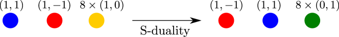
Figure 6: S-duality for the standard components of a $D_{8}$ singularity.

We can now connect the resulting S-dual system of $(p,q)$ 7-branes to our proposed dual by simple monodromy of branes, as shown in figure 7.

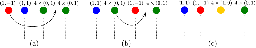
Figure 7: Monodromy converting the S-dual in figure 6 to our proposed dual. We have chosen the branch cuts to run downwards from the 7-branes, as indicated by the dotted lines.

We describe this connection in detail. We take the convention that the branch cut for the monodromy associated to a $(p,q)$ 7-brane runs downwards from the brane. Crossing this branch cut counter-clockwise induces the monodromy:

$$\mathcal{M}_{(p,q)}=\begin{pmatrix}1-pq&p^{2}\\ -q^{2}&1+pq\end{pmatrix}\,.$$ (74)

We divide the stack of 8 $(0,1)$ 7-branes into two stacks of 4 branes each. We now perform the rearrangement shown in figure 7a, taking the $(1,-1)$ 7-brane to the right of the $(1,1)$ 7-brane and the leftmost stack of $(0,1)$ 7-branes. As it moves to its new position it crosses the $(1,1)$ branch cut counter-clockwise, and then the four $(0,1)$ branch cuts. Its new $(p,q)$ labels are thus given by

$$\begin{pmatrix}p^{\prime}\\ q^{\prime}\end{pmatrix}=\mathcal{M}_{(0,1)}^{4}\mathcal{M}_{(1,1)}\begin{pmatrix}1\\ -1\end{pmatrix}=\begin{pmatrix}0&1\\ -1&-2\end{pmatrix}\begin{pmatrix}1\\ -1\end{pmatrix}=\begin{pmatrix}-1\\ 1\end{pmatrix}\,.$$ (75)

The overall sign of the $(p,q)$ charge is not physical, therefore the 7-brane charge is unaltered following this operation. The second step is depicted in figure 7b. We take the leftmost group of $(0,1)$ branes to the right of the $(1,-1)$ brane. In doing this we cross the $(1,-1)$ branch cut counter-clockwise, and thus the $(p,q)$ labels of the $(0,1)$ stack become

$$\begin{pmatrix}p^{\prime}\\ q^{\prime}\end{pmatrix}=\mathcal{M}_{(1,-1)}\begin{pmatrix}0\\ 1\end{pmatrix}=\begin{pmatrix}2&1\\ -1&0\end{pmatrix}\begin{pmatrix}0\\ 1\end{pmatrix}=\begin{pmatrix}1\\ 0\end{pmatrix}\,.$$ (76)

This gives the collection that we proposed, shown in figure 7c.

The above argument was made purely at the level of monodromies. This cannot be the whole story, since eight $D7$ branes atop an $O7^{-}$ plane should naively yield an $SO(16)$ gauge group, distinct from the trivial gauge group expected for an $O7^{+}$ plane. This was already observed in Witten:1997bs , and given an explanation in the context of $K3$ compactifications of F-theory in Bershadsky:1998vn . A general analysis from the type II perspective was then presented in Brunner:2008bi ; Gao:2010ava (see also Distler:2009ri ). From the type II perspective, the type of the orientifold in our configuration will be determined by the sign of the crosscap diagram around the orientifold. As explained in Gao:2010ava , this sign is determined by a parallel section — known as the “crosscap” section — of a line bundle with flat connection. The line bundle and connection are derived from the “twist” line bundle and connection, whose curvature is $B_{2}+\sigma^{\ast}B_{2}$ where $\sigma$ is the orientifold involution. Thus, the orientifold type is indirectly related to the $B_{2}$ discrete torsion $[H]\in H^{3}(X,\tilde{\mathbb{Z}})$.

While in general the crosscap section is not completely determined by $[H]$, for the case of the $\mathbb{C}^{3}/\mathbb{Z}_{3}$ orientifold we argued in §2 that trivial (non-trivial) $[H]$ should correspond to an $O7^{-}$ ($O7^{+}$) wrapping the exceptional divisor. This should follow from the general discussion of Brunner:2008bi ; Gao:2010ava ; it would be interesting to work this out in detail.

5.2 The orientifold transition for $\mathbb{C}^{3}/\mathbb{Z}_{3}$

Given the proposal for the strongly coupled behavior of the $O7^{+}$ above, let us try to obtain the field theory duality conjectured in gauge from the brane description of the system.

The most important change with respect to the flat space case is that tadpole cancellation requires the introduction of some (anti-)branes on top of the orientifold. Consistent configurations are of the form $O7^{+}+4\Omega[1]+2k\,D3s$, with gauge group $U\!Sp(2k+4)\times U(2k)$. Under S-duality, the $O7^{+}$ becomes an $O7^{-}$ with some 7-branes on top. At the quiver point these 7-branes will decay into the standard basis of fractional branes. We conclude that S-duality acts on the wrapped $O7^{+}$ as follows:

$$O7^{+}\xrightarrow{\text{S-duality}}O7^{-}+4\bigl{(}\mathcal{O}(-1)[0]+\mathcal{O}(-2)[2]\bigr{)}+4\bigl{(}\widehat{\mathcal{O}(-1)[0]}+\widehat{\mathcal{O}(-2)[2]}\bigr{)}+n\,D3s\,.$$ (77)

Here $\widehat{\mathscr{E}}$ indicates the S-dual of the brane $\mathscr{E}$, and we have allowed for the inclusion of $n$ $D3$ branes to take into account lower charges induced by curvatures and fluxes. This integer can be determined by imposing $D3$ charge conservation, since $D3$ branes are self-dual under $SL(2,\mathbb{Z})$. Using the expressions for the charges (55) and (44) we obtain $n=-5$. Note that the discussion in the previous section was in terms of mobile 7-branes, so in terms of fractional branes we need to consider $\mathcal{O}(-1)[0]$ and its image $\mathcal{O}(-2)[2]$ together.

We can now treat the whole system. Starting with $O7^{+}+4\Omega[1]+2k\,D3s$, S-duality gives:

$$O7^{-}+4\bigl{(}\mathcal{O}(-1)[0]+\mathcal{O}(-2)[2]\bigr{)}+4\bigl{(}\widehat{\mathcal{O}(-1)[0]}+\widehat{\mathcal{O}(-2)[2]}+\widehat{\Omega[1]}\bigr{)}+(2k-5)\,D3s\,.$$ (78)

Using the fact that the three fractional branes add up to a regular $D3$, which is $SL(2,\mathbb{Z})$ invariant, we can rewrite this configuration as:

$$O7^{-}+4\bigl{(}\mathcal{O}(-1)[0]+\mathcal{O}(-2)[2]\bigr{)}+(2k-1)\,D3s\,.$$ (79)

Taking into account the change in orientifold projection and the discussion in section 4, we therefore find that the full matter content of the theory after the transition it is given by:

$$\begin{array}[]{cc|c}SO(2k-1)&U(2k+3)&SU(3)\\ \hline\cr\overline{\ydiagram}{1}&\ydiagram{1}&\ydiagram{1}\\ 1&\overline{\ydiagram}{1,1}&\ydiagram{1}\end{array}$$ (83)

This is precisely the conjectured field theory dual of theory (63), where ${\tilde{N}}=2k=N-3$.

The main features of this example will generalize to a number of further examples, so let us highlight the primary consequences of the orientifold transition. First of all, we find that under the transition the sign of the orientifold projection changes. This immediately implies that $SO$ and $U\!Sp$ groups get exchanged, while $SU$ groups stay invariant. Similarly, symmetric and antisymmetric representations get exchanged. This agrees perfectly with the features of the duality that we are proposing.

The orientifold transition picture also naturally explains the change in rank of the field theory: it is simply the manifestation of $D3$ charge being conserved. In any given example one can easily calculate the change in rank one needs in order to conserve $D3$ charge, and in all examples that we have checked this change is exactly what is needed for agreement with anomaly matching in the field theory.

The above discussion applies to the case where $[H]$ is changed by S-duality, leading to an orientifold transition. In the case where $[H]$ does not change under S-duality, i.e. where $[H]=[F]$, we expect a self-duality rather than an orientifold transition. In particular, both $[H]=[F]=0$ and $[H]=[F]=1/2$, corresponding to the $SO$ theory for even $N$ and the “$\widetilde{U\!Sp}$” theory, should be self-dual under $S\in SL(2,\mathbb{Z})$. We now describe these self-dualities at the level of the fractional branes.

In the $SO$ case, we have the fractional branes $O7^{-}+4\bigl{(}\mathcal{O}(-1)[0]+\mathcal{O}(-2)[2]\bigr{)}+(N-4)D3s$, but the $O7^{-}+4\bigl{(}\mathcal{O}(-1)[0]+\mathcal{O}(-2)[2]\bigr{)}$ is self-dual (at the level of monodromies) using the same argument as in §5.1, where we merely ignore the rightmost stack of branes in figure 7; thus, the entire configuration of fractional branes is self-dual. In the $U\!Sp$ case, we start with the fractional branes $O7^{+}+4\Omega[1]+\tilde{N}D3s$ and dualize the 7-branes as in the transition above, except that due to the non-vanishing $[H]$ after the duality we treat the resulting 7-brane cluster as the components of an $O7^{+}$ plane. This gives $O7^{+}+4\Omega[1]+nD3s$ for some $n$, where $D3$ charge conservation requires $n=\tilde{N}$. Thus, this configuration is also self-dual, in perfect agreement with the results of §2.

6 Phase II of $\mathbb{C}^{3}/\mathbb{Z}_{3}$

We will now compare the orientifold transition picture we just discussed with the predictions of field theory in a related but illustrative example, the theory Seiberg dual Seiberg:1994pq ; Intriligator:1995id to that of branes at $\mathbb{C}^{3}/\mathbb{Z}_{3}$, leaving the discussion of more involved singularities for the upcoming strings-all .

6.1 Field theory

Figure 8: Seiberg dual of the $\mathbb{C}^{3}/\mathbb{Z}_{3}$ orbifold theory. We have indicated the involution we want to study by the dashed line.

Let us do a Seiberg duality on the top node of the quiver shown in figure 8. This leads to an $SU(2N)\times SU(N)^{2}$ gauge theory that, following the procedure given in Franco:2007ii ; gauge , can be orientifolded as indicated by the dashed line in figure 8. There are two anomaly-free possibilities:

	$SO(2(N+4))$	$SU(N)$	$SU(3)$	$U(1)_{R}$	$\mathbb{Z}_{3}$
$A^{i}$	$\ydiagram{1}$	$\ydiagram{1}$	$\ydiagram{1}$	$\frac{1}{3}-\frac{2}{N}$	$\omega_{3N}$
$B^{ij}$	1	$\overline{\ydiagram{2}}$	$\overline{\ydiagram{2}}$	$\frac{4}{3}+\frac{4}{N}$	$\omega_{3N}^{-2}$

with superpotential

$$W=\frac{1}{2}\operatorname{Tr}A_{i}A_{j}B^{ij}$$ (84)

and

	$U\!Sp(2(\tilde{N}-4))$	$SU(\tilde{N})$	$SU(3)$	$U(1)_{R}$	$\mathbb{Z}_{3}$
$\tilde{A}^{i}$	$\ydiagram{1}$	$\ydiagram{1}$	$\ydiagram{1}$	$\frac{1}{3}+\frac{2}{\tilde{N}}$	$\omega_{3\tilde{N}}$
$\tilde{B}^{ij}$	1	$\overline{\ydiagram{1,1}}$	$\overline{\ydiagram{2}}$	$\frac{4}{3}-\frac{4}{\tilde{N}}$	$\omega_{3\tilde{N}}^{-2}$

with superpotential

$$\tilde{W}=\frac{1}{2}\operatorname{Tr}\tilde{A}_{i}\tilde{A}_{j}\tilde{B}^{ij},$$ (85)

where $\omega_{n}\equiv e^{2\pi i/n}$ and $\tilde{N}$ is even, since for odd $\tilde{N}$ the $U\!Sp(2(\tilde{N}-4))$ gauge group has a Witten anomaly. The discrete symmetry group is $\mathbb{Z}_{3}$ since the third power of the generator given above is contained in the gauge group. For $N$ ($\tilde{N}$) not a multiple of 3 one can show that this $\mathbb{Z}_{3}$ is gauge equivalent to the center of the global $SU(3)$. Thus the global symmetry groups match only if $\tilde{N}$ and $N$ differ by a multiple of 3.

The global symmetry groups and anomalies for these two theories are exactly as for the orientifold theories of phase I (see section 1) and are

$SO(2(N+4))\times SU(N)$ theory:		$U\!Sp(2(\tilde{N}-4))\times SU(\tilde{N})$ theory:
$SU(3)^{3}$ $\frac{3}{2}(N-3)N$ $SU(3)^{2}\times U(1)_{R}$ $-\frac{1}{2}(N-3)N-6$ $U(1)_{R}^{3}$ $\frac{4}{3}(N-3)N-33$ $U(1)_{R}$ $-9$ $SU(3)^{2}\mathbb{Z}_{3}$ 0 $\mathbb{Z}_{3}$ 0		$SU(3)^{3}$ $\frac{3}{2}\tilde{N}(\tilde{N}+3)$ $SU(3)^{2}\times U(1)_{R}$ $-\frac{1}{2}\tilde{N}(\tilde{N}+3)-6$ $U(1)_{R}^{3}$ $\frac{4}{3}\tilde{N}(\tilde{N}+3)-33$ $U(1)_{R}$ $-9$ $SU(3)^{2}\mathbb{Z}_{3}$ 0 $\mathbb{Z}_{3}$ 0

where we write only those discrete anomalies which must match in comparing two dual theories Csaki:1997aw . The anomalies of the two models above match for $\tilde{N}=N-3$.

The two theories given above can also be derived by applying Seiberg duality to the $SO$ or $U\!Sp$ node of the orientifolds of phase I and integrating out the massive matter. In the remainder of this section we derive these two quiver theories explicitly using string theory methods and show that they are related by an orientifold transition.

6.2 String theory

Ordinary Seiberg duality can be understood in the context of the derived category as a tilting of the category Berenstein:2002fi ; Braun:2002sb ; Herzog:2004qw ; Aspinwall:2004vm . In the particular case of the original collection (49) the tilting object giving rise to the Seiberg dual theory can be easily constructed, following the procedure in Herzog:2004qw ; Aspinwall:2004vm , as:

$$\begin{split}\mathsf{P}_{0}^{\prime}&=\mathcal{O}\\ \mathsf{P}_{1}^{\prime}&=\underline{\mathcal{O}(1)^{\oplus 3}}\to\mathcal{O}(2)\\ \mathsf{P}_{2}^{\prime}&=\mathcal{O}(1)\end{split}\,,$$ (86)

where the underline denotes position zero in the complex.

We can construct the basis of fractional branes by mutating the collection $\{\mathsf{P}_{i}^{\prime}\}$ as usual Herzog:2003dj , with the result:

$$\mathcal{C}^{\prime}=\bigl{\{}\mathcal{O},\mathcal{O}(-1)^{\oplus 2}[1],\mathcal{O}(-2)[2]\bigr{\}}\,.$$ (87)

This is the same basis of fractional branes given in Cachazo:2001sg , with the refinement of having the grading in $\mathbb{Z}$, rather than $\mathbb{Z}_{2}$. We have taken two copies of $\mathcal{O}(-1)[1]$ in order to cancel tadpoles. It is easy to compute the spectrum of bifundamentals for this set of fractional branes. We show the resulting quiver in figure 9, which agrees with the quiver in figure 8, as it should.

Figure 9: Basis of branes for the Seiberg dual of the $\mathbb{C}^{3}/\mathbb{Z}_{3}$ orbifold theory.

On the other hand, it is clear from (33) that the ordinary orientifold involution does not act on the fractional branes in the way that we expect, for example:

$$i_{*}\mathcal{O}(-1)[1]\longrightarrow i_{*}(\mathcal{O}(1)\otimes\mathcal{O}(-3))[1]=i_{*}\mathcal{O}(-2)[1]\,,$$ (88)

so this action does not map the $U(N)$ stack to itself. The solution, as advanced in section 4, is to introduce a non-vanishing $B_{2}$ field, in this way modifying the orientifold action to (34). In particular, we will choose $B_{2}=\frac{1}{2}$, or equivalently $\mathcal{L}_{2B_{2}}=\mathcal{O}(1)$. The resulting orientifold then acts as we expect:

$$\begin{split}i_{*}\mathcal{O}(-1)[1]&\longrightarrow i_{*}(\mathcal{O}(1)\otimes\mathcal{O}(-3)\otimes\mathcal{O}(1))[1]=i_{*}\mathcal{O}(-1)[1]\\ i_{*}\mathcal{O}(-2)[2]&\longrightarrow i_{*}(\mathcal{O}(2)\otimes\mathcal{O}(-3)\otimes\mathcal{O}(1))[0]=i_{*}\mathcal{O}\\ i_{*}\mathcal{O}&\longrightarrow i_{*}(\mathcal{O}\otimes\mathcal{O}(-3)\otimes\mathcal{O}(1))[2]=i_{*}\mathcal{O}(-2)[2]\,.\end{split}$$ (89)

The matter content of the orientifolded theory can be derived using the rules in section 4. Assume that we introduce an $O7^{+}$ plane. In order to cancel $D7$ tadpoles we need to introduce 8 $\mathcal{O}(-1)[1]$ planes. We will determine the projection on the invariant branes momentarily; for now let us denote the group on the stack of $\mathcal{O}(-1)[1]$ branes by $G$, which can be either $SO$ or $U\!Sp$. Adding $N$ regular $D3$ branes, we obtain a gauge group $G(2(N+4))\times U(N)$. The chiral multiplet spectrum can be easily obtained using table 1 and the charge vectors

$$\begin{split}e^{-B_{2}}\Gamma(\mathcal{O})&=1+\ell+\frac{5}{8}\ell^{2}\\ e^{-B_{2}}\Gamma(\mathcal{O}(-1)[1])&=-1-\frac{1}{8}\ell^{2}\\ e^{-B_{2}}\Gamma(\mathcal{O}(-2)[2])&=1-\ell+\frac{5}{8}\ell^{2}\\ \Gamma(O7^{+})&=8-\frac{1}{2}\ell^{2}\,,\end{split}$$ (90)

and it is given by:

$$\begin{array}[]{cc|c}SO(2(N+4))&U(N)&SU(3)\\ \hline\cr\overline{\ydiagram}{1}&\ydiagram{1}&\ydiagram{1}\\ 1&\overline{\ydiagram}{2}&\overline{\ydiagram}{2}\end{array}$$ (94)

where we have set $G=SO$ by comparing with the expectation from field theory. (As in the theory before Seiberg duality, a derivation from first principles using the techniques in Brunner:2008bi ; Gao:2010ava should be possible, but we will not attempt to do so here.) Notice also the flavor structure, which can be derived as follows. The modes in the $\ydiagram{1}$ of $U(N)$ come from:

$$\operatorname{Ext}^{1}_{X}(i_{*}\mathcal{O}(-2)[2],i_{*}\mathcal{O}(-1)[1])=\operatorname{Ext}^{0}_{\mathcal{S}}(\mathcal{O}(-2),\mathcal{O}(-1))=\mathbb{C}^{3}\,,$$ (95)

where we have used (39), and the fact that $\operatorname{Ext}^{\bullet}_{\mathcal{S}}(\mathcal{O}(-1),\mathcal{O}(-2))=0$. Furthermore, we can identify geometrically the $SU(3)$ flavor group as $SU(3)$ rotations on the $(z_{1},z_{2},z_{3})$ homogeneous coordinates on $\mathbb{P}^{2}$. We have that $\operatorname{Ext}^{0}_{\mathcal{S}}(\mathcal{O}(-2),\mathcal{O}(-1))=\Gamma(\mathcal{O}(1))$, i.e. the group of sections of $\mathcal{O}(1)$, which are described by polynomials of the form $\sum a_{i}z_{i}$. Thus we can immediately see that the elements transforming in the fundamental of $U(N)$ also transform in the fundamental of $SU(3)$. Similarly, the fields transforming in the $\overline{\ydiagram}{2}$ of $U(N)$ come from:

$$\operatorname{Ext}^{1}_{X}(i_{*}\mathcal{O}[0],i_{*}\mathcal{O}(-2)[2])=\operatorname{Ext}^{0}_{\mathcal{S}}(\mathcal{O}(-2),\mathcal{O})^{\vee}=\mathbb{C}^{6}\,.$$ (96)

One has that $\operatorname{Ext}^{0}_{\mathcal{S}}(\mathcal{O}(-2),\mathcal{O})=\Gamma(\mathcal{O}(2))$. These are polynomials in the homogeneous coordinates of the form $\sum_{ij}c_{ij}z_{i}z_{j}$, which clearly transform in the symmetric representation of the flavor group. Notice, though, that Serre duality gives us the dual of $\Gamma(\mathcal{O}(2))$, which accordingly transforms in the conjugate representation.

Seiberg duality as motion in moduli space

Before going into details of the orientifold transition in this system, we would like to clarify a couple of points in the discussion above. Notice that in the process of Seiberg dualizing we had to introduce half a unit of $B_{2}$ field. It can also be easily seen that if we start with an $O7^{+}$ its Seiberg dual should be an $O7^{-}$. We will now argue that both statements are compatible with (and in the case of the $B_{2}$ field, required from) the usual picture in string theory of Seiberg duality as a motion in Kähler moduli space.

Recall that the quantum moduli space of the $\mathbb{C}^{3}/\mathbb{Z}_{3}$ geometry can be seen as a $\mathbb{P}^{1}$ with three marked points: the quiver point, the large volume point, and a “conifold” point in which a certain D-brane becomes massless. In order to visualize this structure it is convenient, as done in Aspinwall:2004jr , to unfold this sphere into three copies in such a way that the quantum $\mathbb{Z}_{3}$ symmetry of the configuration is manifest. We present the resulting moduli space in figure 10. Due to the orientifold projection this moduli space is restricted to integer and half-integer values of the $B_{2}$ field.

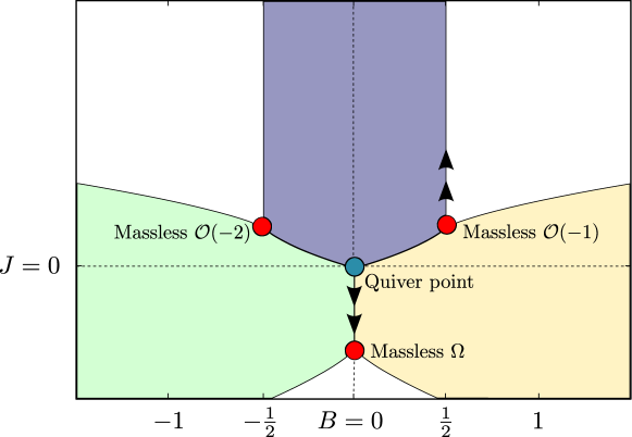
Figure 10: Unfolded moduli space of $\mathbb{C}^{3}/\mathbb{Z}_{3}$ Aspinwall:2004jr . The three colored regions are $\mathbb{Z}_{3}$ images of each other, each region being a copy of the fundamental $\mathbb{P}^{1}$ moduli space. We have denoted the points where the fractional branes become massless by red dots. The path followed in doing Seiberg duality is marked by arrows.

In brane constructions Seiberg duality can often be understood as continuation beyond infinite coupling (see Giveon:1998sr for a nice review of a number of examples). In our configuration this can be achieved as follows. We start from the quiver point at $B_{2}+iJ=0$, and continue towards negative values of $J$ (we depict the motion by arrows in figure 10). At a particular point along this line the invariant brane $\Omega$ becomes massless. Note that due to the $\mathbb{Z}_{3}$ symmetry this point is identified with the point at which $\mathcal{O}(-1)$ becomes massless, so we can continue beyond the singular CFT point along the $B_{2}=\frac{1}{2}$ line. In this picture $\mathcal{O}(-1)$ is the invariant brane which can become massless, and we have a non-vanishing background value for the $B_{2}$ field, perfectly consistent with the description of Seiberg duality above. It is also easy to verify that the collection of branes that we found by tilting is that given by Picard-Lefschetz monodromy around the point where the invariant brane becomes massless, precisely as advocated in the mirror context in Cachazo:2001sg . (We discuss further the mirror picture in appendix A.)

There are a couple of complementary perspectives that could be illuminating. First, notice that in figure 10 there are three branches coming out of the point where $\Omega$ becomes massless. One of the branches is associated with the ordinary large volume orientifold at $B_{2}=0$. The other two branches are ærientifolds of the type that we have discussed in section 4.3. So Seiberg duality in this context involves a change in the orientifold type as we cross a conifold point, a process quite reminiscent of the processes analyzed in Hori:2005bk . In our case the orientifold changes between an ordinary orientifold with $B_{2}=0$ and an ærientifold, which by composition with the quantum symmetry can be turned into an ordinary orientifold of opposite type with $B_{2}=\frac{1}{2}$, as we implicitly did above.

Finally, in the picture of the moduli space as a $\mathbb{P}^{1}$, we have that the orientifold action constrains us to move along the equator. All three special points are located along the equator, and in particular the large volume and conifold points naturally divide the equator into two halves, which we identify with $B_{2}=0$ and $B_{2}=\frac{1}{2}$. Seiberg duality corresponds to crossing from one branch to the other through the conifold point. We illustrate this structure in figure 11.

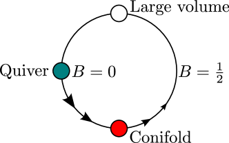
Figure 11: Real moduli space for the orientifolded $\mathbb{C}^{3}/\mathbb{Z}_{3}$. The two possible values for the $B_{2}$ field connect at the singular CFT and the large volume points. Seiberg duality comes from crossing from the quiver side, with $B_{2}=0$, to the side with $B_{2}=\frac{1}{2}$, via the conifold point.

A point which is clear in this last picture is that, as least at the level of motion in Kähler moduli space, the Seiberg dual brane configuration is not supersymmetric, since the quiver point lays in the $B_{2}=0$ half of the real moduli space. It is not difficult to see this explicitly by a direct computation of the periods, which satisfy the Picard-Fuchs equation Candelas:1990rm ; Morrison:1991cd ; BatyrevVariations ; Aspinwall:1993xz

$$\left[\left(z\frac{d}{dz}\right)^{3}+27z\left(z\frac{d}{dz}\right)\left(z\frac{d}{dz}+\frac{1}{3}\right)\left(z\frac{d}{dz}+\frac{2}{3}\right)\right]\Phi=0\,.$$ (97)

A basis of solutions for this equation was found in Aspinwall:1993xz ; Greene:2000ci ; Aspinwall:2004jr . A convenient way of presenting the general form of the solution to this class of problems and doing the analytic continuations is in terms of Meijer $\operatorname{G\!}{}$ functions Greene:2000ci . Choosing the same conventions we chose in writing (52), and introducing a variable $\psi$ given by $-27z=\psi^{-3}$, we obtain:

$$\begin{split}\Phi_{1}&=-\frac{\sqrt{3}}{4\pi^{2}i}\operatorname{G\!}\left[\begin{array}[]{cc|c}\frac{1}{3}&\frac{2}{3}&1\\ 0&0&0\end{array}\right]\!\!\left(-\psi^{-3}\right)\,,\\ \Phi_{2}&=-\frac{\sqrt{3}}{4\pi^{3}}\operatorname{G\!}\left[\begin{array}[]{c|c}\frac{1}{3}\,\,\frac{2}{3}&1\\ 0\,0\,0&-\end{array}\right]\!\!\left(\psi^{-3}\right)\,.\end{split}$$ (98)

Plugging these values in the expression for the central charge (52) and going towards large volume along the $B_{2}=\frac{1}{2}$ line, we obtain the BPS phases shown in figure 12, which clearly show that the Seiberg dual system of branes is not supersymmetric.

Figure 12: Behavior of the phase of the central charge for the fractional branes of the Seiberg dual phases as we go towards large volume along the $B_{2}=\frac{1}{2}$ line, starting from the conifold point at $\psi=e^{2\pi i/3}$ (equivalently $B_{2}=\frac{1}{2}$, $J\approx 0.46$). The central charge of the $\mathcal{O}(-1)[1]$ brane stays real and positive, so we have omitted it from the diagram. The BPS phases asymptote to $\pm\pi$.

We will give further evidence for this statement by carefully analyzing the BPS structure of the mirror in appendix A.

This lack of supersymmetry is clearly something that makes the brane construction of the Seiberg dual somewhat less appealing, but notice that the problem is independent of the presence of the orientifold. Since the mismatch is just at the level of D-terms, we will just assume that the information about the field theory that we get from the brane construction is still reliable, and proceed with the construction. Notice that taking the discussion in this section at face value would then imply a strong/weak duality between a pair of non-supersymmetric theories, different from the example considered in Uranga:1999ib ; Sugimoto:2012rt .

The orientifold transition.

In the previous discussion we have considered the case in which we add an $O7^{+}$ plane. The other possibility consists of adding an $O7^{-}$ plane, which gives the following theory:

$$\begin{array}[]{cc|c}U\!Sp(2(\tilde{N}-4))&U(\tilde{N})&SU(3)\\ \hline\cr\overline{\ydiagram}{1}&\ydiagram{1}&\ydiagram{1}\\ 1&\overline{\ydiagram}{1,1}&\overline{\ydiagram}{2}\end{array}$$ (102)

As before, let us assume that the two configurations are dynamically connected via a strongly coupled orientifold transition. We again expect a process of the form:

$$O7^{+}+4\mathcal{O}(-1)^{\oplus 2}[1]\longleftrightarrow O7^{-}+4(\mathcal{O}+\mathcal{O}(-2)[2])+n\,D3s\,.$$ (103)

Conservation of $D3$ charge then requires:

$$8-\frac{1}{2}\ell^{2}+(-8-\ell^{2})=(-8+\frac{1}{2}\ell^{2})+(8+5\ell^{2})+n\ell^{2}\,,$$ (104)

which implies $n=-7$. Adding $N$ regular branes to the $O7^{+}$ side one obtains the theory (94). After the transition we thus expect the spectrum:

$$O7^{+}+4\mathcal{O}(-1)^{\oplus 2}[1]+N\,D3s\longleftrightarrow O7^{-}+4(\mathcal{O}+\mathcal{O}(-2)[2])+(N-7)\,D3s\,,$$ (105)

i.e. the theory (102) with $\tilde{N}=N-3$, in perfect agreement with the expectations from field theory.

7 Conclusions

In this paper we have argued that the field theory duality presented in gauge admits a very natural embedding in string theory as the action of type IIB S-duality on branes at singularities.

Building on the field theory checks performed in gauge , in this paper we argued that the brane configurations corresponding to the dual theories of gauge source discrete torsions for the NSNS and RR two-forms related by S-duality. Furthermore, we found that the collections of fractional branes constructing the dual theories are in fact S-dual once the $O7^{+}$ is resolved into its $(p,q)$ seven-brane components.

Taken together, these arguments give very strong support to the idea that the $\mathcal{N}=1$ theories we have been discussing are indeed related by strong/weak dualities, and illuminate the physical origin of some of its main features, such as the change in rank and the change between $SO$/$U\!Sp$ groups and symmetric/antisymmetric projections.

There are a number of interesting directions for future work, some of which we now discuss. First, it would be very interesting to extend the ideas in this work to theories without supersymmetry. It was realized in Uranga:1999ib ; Sugimoto:2012rt that the study of a non-supersymmetric version of the brane configuration engineering $\mathcal{N}=4$ SYM would give interesting insight into the strong dynamics of the corresponding non-supersymmetric version of $\mathcal{N}=4$. The same idea should generalize to the much larger class of $\mathcal{N}=1$ duals we have introduced in this paper (and the ones to appear in strings-all ), potentially giving a window into the strongly coupled dynamics of a large class of non-supersymmetric theories.

There are also several formal problems that we have not addressed in this work, but which would be interesting to understand. One such issue is that of K-theory tadpoles. Typically, in the presence of orientifolds, in addition to the usual conditions for cancellation of RR and NSNS tadpoles one should also make sure that certain $\mathbb{Z}_{2}$ valued K-theory tadpoles are canceled Witten:1998cd ; Moore:1999gb ; Diaconescu:2000wy ; Diaconescu:2000wz ; Uranga:2000xp ; LoaizaBrito:2001ux ; GarciaEtxebarria:2005qc . It would be very interesting to have a systematic understanding of such K-theory tadpoles in the configurations we study in this series of papers.

Finally, our discussion of the strongly coupled behavior of the $O7^{+}$ plane was mostly kinematical, focusing on monodromy and charge conservation. It would be very interesting (but probably quite involved) to study the dynamics in more detail, and see that orientifold transitions such as (77) are also dynamically preferred, in the sense that the brane recombinations proceed as we have described.

Appendix A Mirror picture for Seiberg duality on $\mathbb{C}^{3}/\mathbb{Z}_{3}$

We would like to describe the mirror geometry to the $\mathbb{C}^{3}/\mathbb{Z}_{3}$ orbifold. As discussed in detail in Hori:2000kt ; Hori:2000ck (see also Feng:2005gw ), for the purposes of studying BPS objects the mirror can be taken to be a fibration over the complex plane with fiber $\mathbb{C}^{*}\times T^{2}$. Parameterizing the base of the fibration by $z$, the total geometry is given by:

$$uv =z-3\psi$$ (106)

$$y^{2} =x^{3}+\left(\frac{z}{2}\right)^{2}x^{2}+\left(\frac{z}{2}\right)x+\frac{1}{4}\,,$$ (107)

with $u,v\in\mathbb{C}$ and $x,y\in\mathbb{C}^{*}$. The dependence on the Kähler moduli of the original geometry is encoded in the variable $\psi$ introduced above (98). We can recast the elliptic part of the fibration in the usual Weierstrass form by a linear change in variables, getting:

$$y^{2}=x^{3}+f(z)x+g(z)$$ (108)

with

$$\begin{split}f(z)&=-\frac{z}{2}\left(\frac{z^{3}}{24}-1\right)\\ g(z)&=\frac{z^{6}}{864}-\frac{z^{3}}{24}+\frac{1}{4}\,.\end{split}$$ (109)

The resulting discriminant is then given by:

$$\Delta(z)=4f(z)^{3}+27g(z)^{2}=\frac{1}{16}\left(27-z^{3}\right)\,,$$ (110)

and from here we see that the elliptic fiber becomes singular at the three points $z_{*}=3\{1,\,e^{2i\pi/3},\,e^{4i\pi/3}\}$ (associated to the conifold points $\psi=\{1,\,e^{2i\pi/3},\,e^{4i\pi/3}\}$ in the original $\mathbb{C}^{3}/\mathbb{Z}_{3}$ geometry). Finally, the holomorphic 3-form of the geometry can be taken to be:

$$\Omega=\frac{dx}{y}\wedge dz\wedge\frac{du}{u}\,.$$ (111)

A.1 Lattices and elliptic fibrations

In order to compute the structure of special Lagrangian cycles, it is convenient to take the torus from its Weierstrass expression in terms of an equation in $\mathbb{C}^{2}$ to a flat description of the form $\mathbb{C}/\mathbb{L}$, where $\mathbb{L}$ is a lattice generated by the two vectors $2\omega_{1}$ and $2\omega_{3}$ ($\omega_{1}$ and $\omega_{3}$ are called the half-periods, and they are defined up to $SL(2,\mathbb{Z})$ transformations). Notice that in the following we will be working with $\mathbb{L}$, and not just the complex structure $\tau=\omega_{3}/\omega_{1}$ of the torus. This is important in order to explicitly see the special Lagrangian structure of our branes. The technology we will be using in this section is well developed, but we will quickly review it here for the convenience of the reader. We will follow the conventions in DLMFModularFuncs , to which we also refer for further explanations.

The basic map uses the Weierstrass $\wp$ function, defined by:

$$\wp\left(\zeta|\mathbb{L}\right)=\frac{1}{\zeta^{2}}+\sum_{{\omega\in\mathbb{L}\setminus\{0\}}}\left[\frac{1}{(\zeta-\omega)^{2}}-\frac{1}{\omega^{2}}\right]\,.$$ (112)

This is a function of one complex coordinate $\zeta$, and the chosen lattice $\mathbb{L}$. The interest of this function is that it satisfies the differential equation

$$\left(\frac{d\wp}{d\zeta}\right)^{2}=4\wp^{3}-g_{2}\wp-g_{3}\,,$$ (113)

which is clearly the equation of Weierstrass form. The $g_{2}$ and $g_{3}$ coefficients in this equation are determined in terms of $\mathbb{L}$:

$$\begin{split}g_{2}&=60\sum_{\omega\in\mathbb{L}\setminus 0}\frac{1}{\omega^{4}}\\ g_{3}&=140\sum_{\omega\in\mathbb{L}\setminus 0}\frac{1}{\omega^{6}}\,.\end{split}$$ (114)

We can thus map the $x,y$ coordinates to a flat $\zeta$ coordinate if we set $y=\wp^{\prime}$, $x=\sqrt[3]{4}\,\wp$ and choose $\mathbb{L}$ appropriately.

The lattice half-periods can be determined as follows. Consider a Weierstrass fibration rewritten in the following way:

$$y^{2}=4x^{\prime 3}-\widetilde{g_{2}}(z)x^{\prime}-\widetilde{g_{3}}(z)\,.$$ (115)

This is just a change in conventions, with $\widetilde{g_{2}}(z)\equiv-\sqrt[3]{4}f(z)$, $\widetilde{g_{3}}(z)\equiv-g(z)$. The right hand side can be written as $4(x^{\prime}-e_{1})(x^{\prime}-e_{2})(x^{\prime}-e_{3})$. The $e_{i}$ are called the lattice roots. The half-periods are then given by:

$$\begin{split}\omega_{1}&=\frac{\pi}{2\sqrt{e_{1}-e_{3}}}\,_{2}F_{1}\left(\frac{1}{2},\frac{1}{2};1;\frac{e_{2}-e_{3}}{e_{1}-e_{3}}\right)\,,\\ \omega_{3}&=i\frac{\pi}{2\sqrt{e_{1}-e_{3}}}\,_{2}F_{1}\left(\frac{1}{2},\frac{1}{2};1;\frac{e_{1}-e_{2}}{e_{1}-e_{3}}\right)\,,\end{split}$$ (116)

where $\,{}_{2}F_{1}$ denotes the ordinary or Gaussian hypergeometric function. These half-periods define the lattice $\mathbb{L}=\{2\omega_{1}m+2\omega_{3}n,\,\,m,n\in\mathbb{Z}\}$. Choosing this lattice, we have that $\wp(\zeta|\mathbb{L})$ satisfies (113) with $g_{2}=\widetilde{g_{2}}(z)$ and $g_{3}=\widetilde{g_{3}}(z)$. We thus have an embedding into a flat torus, as claimed.

A.2 Special Lagrangian branes at the quiver point

Using the embedding we have just discussed, the holomorphic 3-form simplifies to

$$\Omega=d\zeta\wedge dz\wedge\frac{du}{u}\,.$$ (117)

Branes wrapping a 3-cycle $\mathcal{S}$ are BPS if they are special Lagrangian, which means that $\operatorname{Re}(e^{i\theta}\Omega|_{\mathcal{S}})=0$, for some constant $\theta$. Two sLag branes $\mathcal{S}_{1}$, $\mathcal{S}_{2}$ are mutually supersymmetric if $\theta_{1}=\theta_{2}$. In our case we will be constructing supersymmetric branes wrapping a 1-cycle in the $\mathbb{C}$ base, and a 1-cycle in each of the components of the fiber. We want to construct a supersymmetric system of branes at the quiver point, which is located at $\psi=0$. Equation (106) then reduces to $uv=z$.

The $\mathbb{C}^{*}$ direction is the easiest, we take a 1-cycle parameterized by $u=e^{i\alpha}$, $v=ze^{-i\alpha}$, with $\alpha\in[0,2\pi]$. In this case $du/u=i\,d\alpha$, so the phase of this component of $\Omega$ is constant. In the base we will take the three straight segments that connect $z=0$ with the three points where $\Delta$ vanishes. If the cycle degenerating at $z=z_{*}$ is of type $(p,q)$, we will take a straight (in the $\zeta$-plane) line in the torus fiber, with winding number $(p,q)$. We show the resulting geometry in figure 13.

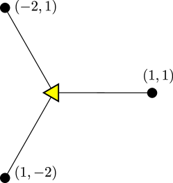
Figure 13: Structure of mirror in the $z$ plane. The central yellow triangle is where the $\mathbb{C}^{*}$ fiber degenerates, and the three black dots outside denote the zeroes of the discriminant. We have also indicated which $(p,q)$ cycle degenerates on which zero, in the particular $SL(2,\mathbb{Z})$ convention used in the text. Finally, the straight lines denote the segments in the base where the sLag branes are to be wrapped.

The total space is thus a $S^{1}\times S^{1}$ fibration over a segment, with each of the fibers degeneration at one of the ends of the segment. It is easy to convince oneself that the topology of the resulting space is $S^{3}$. We will now show that in addition this $S^{3}$ is sLag.

We will start with the horizontal cycle in figure 13, going to the locus where the $(1,1)$ cycle degenerates. The phase of the $dz$ term in $\Omega$ is thus constant, and equal to 0. The structure in the elliptic fiber is more involved, and it is here where the discussion in terms of the lattice $\mathbb{L}$ in the previous section pays off. It is useful to start by looking to the behavior of the complex structure $\tau$ as we go from $z=0$ to the $(1,1)$ degeneration. This can be obtained by computing the inverse of the $j$ function. Introducing Klein’s invariant $J(\tau)=j(\tau)/1728$, one has:

$$J^{-1}(\lambda)=\frac{i(r(\lambda)-s(\lambda))}{r(\lambda)+s(\lambda)}$$ (118)

with

$$r(\lambda) =\Gamma\left(\frac{5}{12}\right)^{2}\,_{2}F_{1}\left(\frac{1}{12},\frac{1}{12};\frac{1}{2};1-\lambda\right)$$ (119)

$$s(\lambda) =2(\sqrt{3}-2)\Gamma\left(\frac{11}{12}\right)^{2}\sqrt{\lambda-1}\,_{2}F_{1}\left(\frac{7}{12},\frac{7}{12};\frac{3}{2};1-\lambda\right)\,.$$ (120)

Plugging in the explicit fibration data (109) for our example, one can easily see that $\tau$ varies as shown in figure 14.

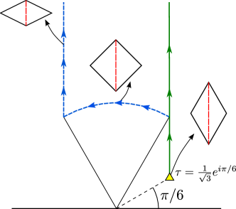
Figure 14: Behavior of $\tau$ as we move along the base. We have depicted the corresponding rhombic lattice cell for various values of $\tau$. The red dashed line denotes the $(1,1)$ cycle wrapped by the brane. The solid green line on the right shows the path of $\tau$ in the natural conventions from the point of view of the rhombic lattice, while the dashed line on the left is an equivalent path along the edge of the fundamental domain, obtained by $\tau\to\tau/(1-\tau)$ for the component with $|\tau|\leq 1$, and $\tau\to\tau-1$ for $|\tau|\geq 1$.

For our purposes the most natural domain for $\tau$ comes from considering the rhombic lattice, and it is shown as the green vertical path in figure 14. Recall, from DLMFModularFuncs , that rhombic lattices are defined by $\omega_{1}$ real and positive, $\operatorname{Im}(\omega_{3})\geq 0$ and $\operatorname{Re}(\omega_{3})=\frac{1}{2}\omega_{1}$. Since conventionally $\tau=\omega_{3}/\omega_{1}$, one automatically has $\operatorname{Re}(\tau)=\frac{1}{2}$.

In these conventions the path is straight, starting from the equianharmonic lattice at $z=0$, with $\tau=e^{i\pi/6}/\sqrt{3}$, and going vertically to infinity, reached at $z=z_{*}$, where the $(1,1)$ cycle degenerates. As we go along the path, the unit cell becomes flatter and flatter in the vertical direction. One can easily verify these statements using the formulas (116).

Of crucial importance for us is that not only is $\tau$ that of a rhombic lattice, but $\omega_{1}$ is real. This means that, no matter our position along the segment in the $z$ plane, the $(1,1)$ cycle in the torus always wraps real values for the flat coordinate $\zeta$, so $d\zeta$ has constant phase, and thus $\Omega$ has constant phase, as we claimed.

Notice that this construction strongly requires working with the whole lattice $\mathbb{L}$, and not just its complex structure $\tau$. If we had defined the torus in the conventional way $\zeta\sim\zeta+1\sim\zeta+\tau$ the $(1,1)$ cycle would have had slope $\arctan(\operatorname{Im}(\tau)/(1+\operatorname{Re}(\tau)))$, which can easily be seen to vary non-trivially along the segment in the base.

Let us consider the other two $D6$ branes, going from the origin to the discriminant points $z_{*}=3\{e^{2i\pi/3},\,e^{4i\pi/3}\}$. For simplicity let us consider $z_{*}=3e^{2i\pi/3}$ only, the other point works similarly. The first observation is that the segment in the base can be obtained simply by multiplying the segment we just considered by $\beta\equiv e^{2i\pi/3}$ (i.e. it is just a rotation by $120^{\circ}$). From the expression for $f$ and $g$ in (109) it is clear that upon doing this rotation $f\to\beta f$, $g\to g$. In addition, since $j(\tau)\sim f^{3}/\Delta$, one has that the $j$ function is invariant upon doing this rotation, and this implies (by taking the inverse via (118)) that $\tau$ is unaffected by the rotation. Since now we want to consider $(p,q)$ cycles different from $(1,1)$ this would immediately imply (if we just look to $\tau$) that the phase of $\Omega$ would vary as we move along the base, making the cycle non-calibrated.

The resolution is as before looking to $\mathbb{L}$, instead of just $\tau$. In particular, from (114) one easily sees that $\omega_{i}\to\beta^{-1}\omega_{i}$, so the lattice is rotated in the direction opposite to the rotation in the base. This also implies that, as we move towards $z_{*}$, the equianharmonic lattice will start deforming, in a way that is a $\beta^{-1}$ rotation of the deformation we saw before. In particular the brane related by a $\beta^{-1}$ rotation to the $(1,1)$ brane will be the one with constant slope. As depicted in figure 15, in this particular case the brane of interest is the $(-2,1)$ brane.

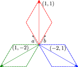
Figure 15: Three fundamental cells of the equianharmonic lattice, rotated by powers of $\beta$. We have drawn the cycles wrapped by the $D6$ branes.

This argument also shows that in addition to each brane being individually sLag, the three branes are also mutually supersymmetric, since the rotation in the base and in the fiber are precisely opposite.

A.3 The orientifold configuration and Seiberg duality

Let us now discuss the mirror to the discussion in section 6, once we introduce the orientifold and move in moduli space. Looking to figure 13, or by recalling that in the $\mathbb{C}^{3}/\mathbb{Z}_{3}$ orbifold the orientifold acted as $\psi\to\overline{\psi}$, it is clear that the mirror orientifold acts on the $z$ plane by conjugation: $z\to\overline{z}$. Similarly, it acts by complex conjugation on the flat torus $\mathbb{C}/\mathbb{L}$, which in terms of cycles can be easily seen to correspond to a $(a,b)\leftrightarrow(b,a)$ exchange for the basis of cycles that we have chosen for the rhombic cell. The net effect is that the $(1,-2)$ and $(-2,1)$ branes are exchanged, while the $(1,1)$ brane stays invariant.

In the current picture Seiberg duality comes from changing the value of $\psi$ in (106) Cachazo:2001sg . A possible choice is to move in moduli space to a point where the $\mathbb{C}^{*}$ fiber degenerates at some real value of $z$ larger than 3. The moduli space of the configuration is now restricted to moving $z$ along the real axis, so exactly as in the IIB picture, we necessarily pass through the singular $z=3$ point when doing this.

It is interesting to look to the detailed behavior of the torus lattice as we move along the real line, we depict this in figure 16.

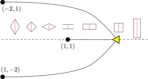
Figure 16: The Seiberg dual configuration. We have depicted schematically the structure of the special Lagrangian branes and the behavior of the elliptic fiber.

On the side of the quiver point the lattice cell has rhombic structure. This cell becomes singular at the conifold point, and on the opposite side of the real line a rectangular lattice emerges. This is presumably the mirror manifestation of the $B_{2}=0$ to $B_{2}=\frac{1}{2}$ transition on the IIB side. In a natural basis for the rectangular lattice the invariant brane wraps the $(1,0)$ cycle, while the $(-1,2)$ and $(-2,1)$ branes wrap the $(1,3)$ and $(1,-3)$ cycles respectively. The orientifold acts on the $z$ plane as before, and acts on the rectangular lattice by sending $(p,q)$ cycles to $(p,-q)$ cycles (i.e. inverting the sign of the second coordinate).

References

- (1) I. Garcia-Etxebarria, B. Heidenreich, and T. Wrase, New dualities from orientifold transitions — Part I: Field Theory, arXiv:1210.7799.
- (2) E. Witten, Baryons and branes in anti-de Sitter space, JHEP 9807 (1998) 006, [hep-th/9805112].
- (3) I. Garcia-Etxebarria, B. Heidenreich, and T. Wrase, New dualities from orientifold transitions — Part III: Non-orbifold singularities, to appear.
- (4) M. Bianchi, G. Inverso, J. F. Morales, and D. R. Pacifici, Unoriented Quivers with Flavour, arXiv:1307.0466.
- (5) C. Vafa, Modular Invariance and Discrete Torsion on Orbifolds, Nucl.Phys. B273 (1986) 592.
- (6) C. Vafa and E. Witten, On orbifolds with discrete torsion, J.Geom.Phys. 15 (1995) 189–214, [hep-th/9409188].
- (7) M. R. Douglas, D-branes and discrete torsion, hep-th/9807235.
- (8) M. R. Douglas and B. Fiol, D-branes and discrete torsion. 2., JHEP 0509 (2005) 053, [hep-th/9903031].
- (9) E. R. Sharpe, Discrete torsion, Phys.Rev. D68 (2003) 126003, [hep-th/0008154].
- (10) E. R. Sharpe, Recent developments in discrete torsion, Phys.Lett. B498 (2001) 104–110, [hep-th/0008191].
- (11) E. Sharpe, Notes on discrete torsion in orientifolds, J.Geom.Phys. 61 (2011) 1017–1032, [arXiv:0908.0087].
- (12) P. Goddard, J. Nuyts, and D. I. Olive, Gauge Theories and Magnetic Charge, Nucl.Phys. B125 (1977) 1.
- (13) C. Montonen and D. I. Olive, Magnetic Monopoles as Gauge Particles?, Phys.Lett. B72 (1977) 117.
- (14) H. Osborn, Topological Charges for N=4 Supersymmetric Gauge Theories and Monopoles of Spin 1, Phys.Lett. B83 (1979) 321.
- (15) N. J. Hitchin, Lectures on special Lagrangian submanifolds, math/9907034.
- (16) A. Kapustin, D-branes in a topologically nontrivial B field, Adv.Theor.Math.Phys. 4 (2000) 127–154, [hep-th/9909089].
- (17) V. Braun and J. Stefanski, B., Orientifolds and K theory, hep-th/0206158.
- (18) J. Distler, D. S. Freed, and G. W. Moore, Orientifold Precis, arXiv:0906.0795.
- (19) J. Distler, D. S. Freed, and G. W. Moore, Spin structures and superstrings, arXiv:1007.4581. Isadore Singer on the occasion of his 85th birthday.
- (20) D. S. Freed and E. Witten, Anomalies in string theory with D-branes, Asian J.Math 3 (1999) 819, [hep-th/9907189].
- (21) A. Hatcher, Algebraic Topology. Cambridge University Press, 2002. http://www.math.cornell.edu/~hatcher/AT/ATpage.html.
- (22) Y. Hyakutake, Y. Imamura, and S. Sugimoto, Orientifold planes, type I Wilson lines and nonBPS D-branes, JHEP 0008 (2000) 043, [hep-th/0007012].
- (23) D. A. Cox, J. B. Little, and H. K. Schenk, Toric Varieties, vol. 124 of Graduate Studies in Mathematics. American Mathematical Society, 2011.
- (24) J. M. Garcia, “Toric varieties in a nutshell.” http://www.maths.ed.ac.uk/~jmartinezgarcia/papers/toricNutshell.pdf, 2010.
- (25) K. D. Kennaway, Brane Tilings, Int.J.Mod.Phys. A22 (2007) 2977–3038, [arXiv:0706.1660].
- (26) D. A. Cox, The Homogeneous coordinate ring of a toric variety, revised version, alg-geom/9210008.
- (27) A. Hanany and K. D. Kennaway, Dimer models and toric diagrams, hep-th/0503149.
- (28) S. Franco, A. Hanany, K. D. Kennaway, D. Vegh, and B. Wecht, Brane dimers and quiver gauge theories, JHEP 0601 (2006) 096, [hep-th/0504110].
- (29) S. Franco, A. Hanany, D. Krefl, J. Park, A. M. Uranga, and D. Vegh, Dimers and orientifolds, JHEP 0709 (2007) 075, [arXiv:0707.0298].
- (30) S. Franco and G. Torroba, Gauge theories from D7-branes over vanishing 4-cycles, JHEP 1101 (2011) 017, [arXiv:1010.4029].
- (31) M. Bianchi, G. Pradisi, and A. Sagnotti, Toroidal compactification and symmetry breaking in open string theories, Nucl.Phys. B376 (1992) 365–386.
- (32) E. G. Gimon and J. Polchinski, Consistency conditions for orientifolds and d manifolds, Phys.Rev. D54 (1996) 1667–1676, [hep-th/9601038].
- (33) M. Berkooz, R. G. Leigh, J. Polchinski, J. H. Schwarz, N. Seiberg, et. al., Anomalies, dualities, and topology of D = 6 N=1 superstring vacua, Nucl.Phys. B475 (1996) 115–148, [hep-th/9605184].
- (34) C. Angelantonj, M. Bianchi, G. Pradisi, A. Sagnotti, and Y. Stanev, Chiral asymmetry in four-dimensional open string vacua, Phys.Lett. B385 (1996) 96–102, [hep-th/9606169].
- (35) G. Aldazabal, A. Font, L. E. Ibanez, A. Uranga, and G. Violero, Nonperturbative heterotic D = 6, D = 4, N=1 orbifold vacua, Nucl.Phys. B519 (1998) 239–281, [hep-th/9706158].
- (36) I. Antoniadis, G. D’Appollonio, E. Dudas, and A. Sagnotti, Partial breaking of supersymmetry, open strings and M theory, Nucl.Phys. B553 (1999) 133–154, [hep-th/9812118].
- (37) P. G. Camara, E. Dudas, T. Maillard, and G. Pradisi, String instantons, fluxes and moduli stabilization, Nucl.Phys. B795 (2008) 453–489, [arXiv:0710.3080].
- (38) M. Bianchi, F. Fucito, and J. F. Morales, Dynamical supersymmetry breaking from unoriented D-brane instantons, JHEP 0908 (2009) 040, [arXiv:0904.2156].
- (39) C. Csaki and H. Murayama, Discrete anomaly matching, Nucl.Phys. B515 (1998) 114–162, [hep-th/9710105].
- (40) K. A. Intriligator and B. Wecht, The Exact superconformal R symmetry maximizes a, Nucl.Phys. B667 (2003) 183–200, [hep-th/0304128].
- (41) Z. Kakushadze, Gauge theories from orientifolds and large N limit, Nucl.Phys. B529 (1998) 157–179, [hep-th/9803214].
- (42) R. P. Thomas, Derived categories for the working mathematician, math/0001045.
- (43) E. R. Sharpe, D-branes, derived categories, and Grothendieck groups, Nucl.Phys. B561 (1999) 433–450, [hep-th/9902116].
- (44) M. R. Douglas, D-branes, categories and supersymmetry, J.Math.Phys. 42 (2001) 2818–2843, [hep-th/0011017].
- (45) E. Sharpe, Lectures on D-branes and sheaves, hep-th/0307245.
- (46) P. S. Aspinwall, D-branes on Calabi-Yau manifolds, hep-th/0403166.
- (47) M. R. Douglas, B. Fiol, and C. Romelsberger, The Spectrum of BPS branes on a noncompact Calabi-Yau, JHEP 0509 (2005) 057, [hep-th/0003263].
- (48) F. Cachazo, B. Fiol, K. A. Intriligator, S. Katz, and C. Vafa, A Geometric unification of dualities, Nucl.Phys. B628 (2002) 3–78, [hep-th/0110028].
- (49) M. Wijnholt, Large volume perspective on branes at singularities, Adv.Theor.Math.Phys. 7 (2004) 1117–1153, [hep-th/0212021].
- (50) C. P. Herzog and J. Walcher, Dibaryons from exceptional collections, JHEP 0309 (2003) 060, [hep-th/0306298].
- (51) P. S. Aspinwall and I. V. Melnikov, D-branes on vanishing del Pezzo surfaces, JHEP 0412 (2004) 042, [hep-th/0405134].
- (52) M. Wijnholt, Parameter space of quiver gauge theories, Adv.Theor.Math.Phys. 12 (2008) [hep-th/0512122].
- (53) A. Hanany, C. P. Herzog, and D. Vegh, Brane tilings and exceptional collections, JHEP 0607 (2006) 001, [hep-th/0602041].
- (54) D.-E. Diaconescu, A. Garcia-Raboso, R. L. Karp, and K. Sinha, D-Brane Superpotentials in Calabi-Yau Orientifolds, Adv.Theor.Math.Phys. 11 (2007) 471–516, [hep-th/0606180].
- (55) A. I. Bondal, Helices, representations of quivers and koszul algebras, in Helices and Vector Bundles (A. N. Rudakov, ed.), no. 148 in London Mathematical Society Lecture Note Series, pp. 75–96. Cambridge University Press, 1990.
- (56) B. Feng, A. Hanany, Y. H. He, and A. Iqbal, Quiver theories, soliton spectra and Picard-Lefschetz transformations, JHEP 0302 (2003) 056, [hep-th/0206152].
- (57) S. H. Katz and E. Sharpe, D-branes, open string vertex operators, and Ext groups, Adv.Theor.Math.Phys. 6 (2003) 979–1030, [hep-th/0208104].
- (58) D. Cox and S. Katz, Mirror Symmetry and Algebraic Geometry. Mathematical Surveys and Monographs. American Mathematical Society, 1999.
- (59) K. Hori, S. Katz, A. Klemm, R. Pandharipande, R. Thomas, C. Vafa, R. Vakil, and E. Zaslow, Mirror Symmetry. Clay Mathematics Monographs. American Mathematical Society, 2003.
- (60) P. Seidel and R. P. Thomas, Braid group actions on derived categories of coherent sheaves, ArXiv Mathematics e-prints (Jan., 2000) [math/0001].
- (61) R. Blumenhagen, L. Goerlich, B. Kors, and D. Lust, Noncommutative compactifications of type I strings on tori with magnetic background flux, JHEP 0010 (2000) 006, [hep-th/0007024].
- (62) L. E. Ibanez, F. Marchesano, and R. Rabadan, Getting just the standard model at intersecting branes, JHEP 0111 (2001) 002, [hep-th/0105155].
- (63) M. Cvetič, G. Shiu, and A. M. Uranga, Three family supersymmetric standard - like models from intersecting brane worlds, Phys.Rev.Lett. 87 (2001) 201801, [hep-th/0107143].
- (64) M. Cvetič, G. Shiu, and A. M. Uranga, Chiral four-dimensional N=1 supersymmetric type 2A orientifolds from intersecting D6 branes, Nucl.Phys. B615 (2001) 3–32, [hep-th/0107166].
- (65) F. Marchesano, Progress in D-brane model building, Fortsch.Phys. 55 (2007) 491–518, [hep-th/0702094].
- (66) I. Brunner and M. Herbst, Orientifolds and D-branes in N=2 gauged linear sigma models, Adv.Theor.Math.Phys. 14 (2010) [arXiv:0812.2880].
- (67) D. Gao and K. Hori, On The Structure Of The Chan-Paton Factors For D-Branes In Type II Orientifolds, arXiv:1004.3972.
- (68) M. Wijnholt, Geometry of Particle Physics, Adv.Theor.Math.Phys. 13 (2009) [hep-th/0703047].
- (69) P. Candelas, X. C. De La Ossa, P. S. Green, and L. Parkes, A Pair of Calabi-Yau manifolds as an exactly soluble superconformal theory, Nucl.Phys. B359 (1991) 21–74.
- (70) K. Hori, A. Iqbal, and C. Vafa, D-branes and mirror symmetry, hep-th/0005247.
- (71) I. Brunner, K. Hori, K. Hosomichi, and J. Walcher, Orientifolds of Gepner models, JHEP 0702 (2007) 001, [hep-th/0401137].
- (72) R. Minasian and G. W. Moore, K theory and Ramond-Ramond charge, JHEP 9711 (1997) 002, [hep-th/9710230].
- (73) A. Sen, Stable nonBPS states in string theory, JHEP 9806 (1998) 007, [hep-th/9803194].
- (74) A. Sen, Stable nonBPS bound states of BPS D-branes, JHEP 9808 (1998) 010, [hep-th/9805019].
- (75) A. Sen, Tachyon condensation on the brane anti-brane system, JHEP 9808 (1998) 012, [hep-th/9805170].
- (76) O. Bergman and M. R. Gaberdiel, Stable nonBPS D particles, Phys.Lett. B441 (1998) 133–140, [hep-th/9806155].
- (77) A. Sen, SO(32) spinors of type I and other solitons on brane - anti-brane pair, JHEP 9809 (1998) 023, [hep-th/9808141].
- (78) M. Srednicki, IIB or not IIB, JHEP 9808 (1998) 005, [hep-th/9807138].
- (79) E. Witten, D-branes and K theory, JHEP 9812 (1998) 019, [hep-th/9810188].
- (80) A. Sen, NonBPS states and Branes in string theory, hep-th/9904207.
- (81) J. H. Schwarz, TASI lectures on nonBPS D-brane systems, hep-th/9908144.
- (82) K. Olsen and R. J. Szabo, Constructing D-branes from K theory, Adv.Theor.Math.Phys. 3 (1999) 889–1025, [hep-th/9907140].
- (83) J. Evslin, What does(n’t) K-theory classify?, hep-th/0610328.
- (84) M. Frau, L. Gallot, A. Lerda, and P. Strigazzi, Stable nonBPS D-branes in type I string theory, Nucl.Phys. B564 (2000) 60–85, [hep-th/9903123].
- (85) O. Loaiza-Brito and A. M. Uranga, The Fate of the type I nonBPS D7-brane, Nucl.Phys. B619 (2001) 211–231, [hep-th/0104173].
- (86) K. Dasgupta and S. Mukhi, Orbifolds of M theory, Nucl.Phys. B465 (1996) 399–412, [hep-th/9512196].
- (87) E. Witten, Five-branes and M theory on an orbifold, Nucl.Phys. B463 (1996) 383–397, [hep-th/9512219].
- (88) E. Witten, New ‘gauge’ theories in six-dimensions, JHEP 9801 (1998) 001, [hep-th/9710065].
- (89) A. M. Uranga, Towards mass deformed and gauge theories from brane configurations, Nucl.Phys. B526 (1998) 241–277, [hep-th/9803054].
- (90) K. Hori, Consistency condition for five-brane in M theory on orbifold, Nucl.Phys. B539 (1999) 35–78, [hep-th/9805141].
- (91) E. G. Gimon, On the M theory interpretation of orientifold planes, hep-th/9806226.
- (92) S. Sethi, A Relation between gauge theories in three-dimensions, JHEP 9811 (1998) 003, [hep-th/9809162].
- (93) M. Berkooz and A. Kapustin, New IR dualities in supersymmetric gauge theory in three-dimensions, JHEP 9902 (1999) 009, [hep-th/9810257].
- (94) A. Hanany, B. Kol, and A. Rajaraman, Orientifold points in M theory, JHEP 9910 (1999) 027, [hep-th/9909028].
- (95) A. M. Uranga, Comments on nonsupersymmetric orientifolds at strong coupling, JHEP 0002 (2000) 041, [hep-th/9912145].
- (96) A. Hanany and B. Kol, On orientifolds, discrete torsion, branes and M theory, JHEP 0006 (2000) 013, [hep-th/0003025].
- (97) K. Landsteiner and E. Lopez, New curves from branes, Nucl.Phys. B516 (1998) 273–296, [hep-th/9708118].
- (98) E. Witten, Toroidal compactification without vector structure, JHEP 9802 (1998) 006, [hep-th/9712028].
- (99) M. Bershadsky, T. Pantev, and V. Sadov, F theory with quantized fluxes, Adv.Theor.Math.Phys. 3 (1999) 727–773, [hep-th/9805056].
- (100) A. Sen, Orientifold limit of F theory vacua, Phys.Rev. D55 (1997) 7345–7349, [hep-th/9702165].
- (101) T. Banks, M. R. Douglas, and N. Seiberg, Probing F theory with branes, Phys.Lett. B387 (1996) 278–281, [hep-th/9605199].
- (102) N. Seiberg, Electric - magnetic duality in supersymmetric nonAbelian gauge theories, Nucl.Phys. B435 (1995) 129–146, [hep-th/9411149].
- (103) K. A. Intriligator and N. Seiberg, Duality, monopoles, dyons, confinement and oblique confinement in supersymmetric SO(N(c)) gauge theories, Nucl.Phys. B444 (1995) 125–160, [hep-th/9503179].
- (104) D. Berenstein and M. R. Douglas, Seiberg duality for quiver gauge theories, hep-th/0207027.
- (105) V. Braun, On Berenstein-Douglas-Seiberg duality, JHEP 0301 (2003) 082, [hep-th/0211173].
- (106) C. P. Herzog, Seiberg duality is an exceptional mutation, JHEP 0408 (2004) 064, [hep-th/0405118].
- (107) A. Giveon and D. Kutasov, Brane dynamics and gauge theory, Rev.Mod.Phys. 71 (1999) 983–1084, [hep-th/9802067].
- (108) K. Hori, K. Hosomichi, D. C. Page, R. Rabadan, and J. Walcher, Non-perturbative orientifold transitions at the conifold, JHEP 0510 (2005) 026, [hep-th/0506234].
- (109) D. R. Morrison, Picard-Fuchs equations and mirror maps for hypersurfaces, hep-th/9111025.
- (110) V. V. Batyrev, Variations of the mixed hodge structure of affine hypersurfaces in algebraic tori, Duke Math. J. 69 (1993), no. 2 349–409.
- (111) P. S. Aspinwall, B. R. Greene, and D. R. Morrison, Measuring small distances in N=2 sigma models, Nucl.Phys. B420 (1994) 184–242, [hep-th/9311042].
- (112) B. R. Greene and C. Lazaroiu, Collapsing D-branes in Calabi-Yau moduli space. 1., Nucl.Phys. B604 (2001) 181–255, [hep-th/0001025].
- (113) S. Sugimoto, Confinement and Dynamical Symmetry Breaking in non-SUSY Gauge Theory from S-duality in String Theory, Prog. Theor. Phys. 128 (2012) , 1175–1209, [arXiv:1207.2203].
- (114) G. W. Moore and E. Witten, Selfduality, Ramond-Ramond fields, and K theory, JHEP 0005 (2000) 032, [hep-th/9912279].
- (115) D.-E. Diaconescu, G. W. Moore, and E. Witten, E(8) gauge theory, and a derivation of K theory from M theory, Adv.Theor.Math.Phys. 6 (2003) 1031–1134, [hep-th/0005090].
- (116) D.-E. Diaconescu, G. W. Moore, and E. Witten, A Derivation of K theory from M theory, hep-th/0005091.
- (117) A. M. Uranga, D-brane probes, RR tadpole cancellation and K theory charge, Nucl.Phys. B598 (2001) 225–246, [hep-th/0011048].
- (118) I. Garcia-Etxebarria and A. M. Uranga, From F/M-theory to K-theory and back, JHEP 0602 (2006) 008, [hep-th/0510073].
- (119) K. Hori and C. Vafa, Mirror symmetry, hep-th/0002222.
- (120) B. Feng, Y.-H. He, K. D. Kennaway, and C. Vafa, Dimer models from mirror symmetry and quivering amoebae, Adv.Theor.Math.Phys. 12 (2008) 3, [hep-th/0511287].
- (121) W. P. Reinhardt and P. L. Walker, “Weierstrass Elliptic and Modular Functions.” Digital Library of Mathematical Functions. Release 2012-03-23. National Institute of Standards and Technology from http://dlmf.nist.gov/23.