WU-HEP-13-02 KUNS-2454 Flavor landscape of 10D SYM theory
with magnetized extra dimensions

1 Introduction

The standard model (SM) of elementary particles is a quite successful theory, consistent with all the experimental data obtained so far with a great accuracy. However, it does not describe gravitational interactions of elementary particles that could play an important role at the very beginning of our universe. Superstring theories in ten-dimensional (10D) spacetime are almost the only known candidates for ultimate unification theory of elementary particles including gravitational interactions. Supersymmetric Yang-Mills (SYM) theories in various spacetime dimensions appear as low energy effective theories of superstring compactifications with or without D-branes. That is quite attractive from the phenomenological viewpoint as well as the theoretical viewpoint. Indeed, based on SYM effective theories, various phenomenological aspects of superstring models have been studied so far. (See for a review [1].) It is an interesting possibility that the SM is embedded in one of such SYM theories, that is, the SM is realized as a low energy effective theory of the superstring theories. In such a string model building, it is a key issue how to break higher-dimensional supersymmetry and to obtain a four-dimensional (4D) chiral spectrum. String compactifications on the Calabi-Yau (CY) space provide a general procedure for such a purpose. However, the metric of a generic CY space is difficult to be determined analytically. That makes phenomenological studies qualitative, but not quantitative.

It is quite interesting that even simple toroidal compactifications but with magnetic fluxes in extra dimensions induce 4D chiral spectra starting with higher-dimensional SYM theories as well as superstring theories [2, 3]. The higher-dimensional supersymmetry such as ${\cal N}=4$ in terms of supercharges in 4D spacetime is broken by magnetic fluxes down to 4D ${\cal N}=0$, $1$ or $2$ depending on the configuration of fluxes. The number of the chiral zero-modes is determined by the magnitude of magnetic fluxes. A phenomenologically attractive feature is that these chiral zero modes localize at different points in magnetized extra dimensions. The overlap integrals of localized wavefunctions yield hierarchical couplings in the 4D effective theory of these zero modes. That could explain, e.g., observed hierarchical masses and mixing angles of the quarks and the leptons [4]. Furthermore, higher-order couplings can also be computed as the overlap integrals of wavefunctions [5]. A theoretically attractive point here is that many peculiar properties of the SM, such as the 4D chirality, the number of generations, the flavor symmetries [6, 7, 8, 9] and potentially hierarchical Yukawa couplings all could be determined by the magnetic fluxes.

In our previous works [10, 11], we have presented 4D ${\cal N}=1$ superfield description of 10D SYM theories compactified on magnetized tori which preserve the ${\cal N}=1$ supersymmetry, and derived 4D effective action for massless zero-modes written in the ${\cal N}=1$ superspace. It makes easy to construct models and analysis that. Thanks to that, we have constructed a three-generation model of quark and lepton chiral superfields based on a toroidal compactification of the 10D SYM theory with certain magnetic fluxes in extra dimensions preserving a 4D ${\cal N}=1$ supersymmetry. The low-energy effective theory contains the minimal supersymmetric standard model (MSSM) particle contents, where the three generation structure of chiral matter fields is originated by the magnitudes of fluxes, and it gives a semi-realistic pattern of hierarchical masses and mixing angles of the quarks and the leptons [11]. Furthermore, we estimated the size of supersymmetric flavor violations.

One typical model has been studied in our previous works, however, there may be other possibilities for particle physics models based on a 10D SYM theory compactified on three factorizable tori $T^{2}\times T^{2}\times T^{2}$ where magnetic fluxes are present in the YM sector. In this paper, we search systematically such possibilities to obtain models which contains the MSSM and study the flavor landscape of 10D magnetized SYM theories, requiring full rank Yukawa matrices among three generations of quarks and leptons. We include possibilities of non-factorizable magnetic fluxes [3, 12, 13]. (See also [14].) We also consider the $T^{6}/Z_{2}$ orbifold with magnetic fluxes as the geometrical background [15].^,

The sections are organized as follows. In Sec. 2, a superfield description of the 10D SYM theory is briefly reviewed based on Ref. [10], which allows the systematic introduction of magnetic fluxes in extra dimensions preserving the ${\cal N}=1$ supersymmetry. Then, we introduce (factorizable) magnetic fluxes and search systematically their proper configurations to construct models that contains the spectrum of the MSSM with or without orbifold projection in Sec. 3. In Sec. 4, we consider magnetic fluxes which cross over two tori. It gives possibilities of more various model building to us. Including such nonfactorizable fluxes, we carry out a systematic search with or without orbifold projection. Sec. 5 is devoted to conclusions and discussions. In Appendix A, we show one $Z_{2}$ orbifold model, where most of exotic zero-modes are projected out. In Appendix B, we show explicitly Yukawa matrices in one type1 model shown in Sec. 4.3

2 The 10D SYM theory in ${\cal N}=1$ superspace

We consider a compactification of 10D SYM theory on 4D flat Minkowski spacetime times a product of factorizable three tori $T^{2}\times T^{2}\times T^{2}$ and use a superfield description suitable for such a compactification with magnetic fluxes preserving 4D ${\cal N}=1$ supersymmetry. Basically, we assume that the compactification scale is around the GUT or Planck scale, although application to other compactifications is straightforward. We mostly follow the notations and the conventions adopted in our previous works [10, 11]. Here, we briefly review only essential points for this work.

We decompose the 10D vector (gauge) field $A_{M}$ into the 4D vector field $A_{\mu}$ and three complex fields $A_{i}$ $(i=1,2,3)$. Also the 10D Majorana-Weyl spinor field $\lambda$ is decomposed into four 4D Weyl spinor fields $\lambda_{0}$ and $\lambda_{i}$ $(i=1,2,3)$. For 4D positive chirality, these spinor fields $\lambda_{0}$, $\lambda_{1}$, $\lambda_{2}$, and $\lambda_{3}$ have the 6D chiralities, $(+,+,+)$, $(+,-,-)$, $(-,+,-)$, and $(-,-,+)$ on $T^{2}\times T^{2}\times T^{2}$. The 10D SYM theory possesses ${\cal N}=4$ supersymmetry counted in terms of 4D supercharges. The YM vector and spinor fields, $A_{M}$ and $\lambda$, are decomposed into (on-shell) 4D ${\cal N}=1$ single vector and triple chiral multiplets, ${\bm{V}}=\left\{A_{\mu},\lambda_{0}\right\}$ and ${\bm{\phi}}_{i}\ =\ \left\{A_{i},\lambda_{i}\right\}$ $(i=1,2,3)$.

The above ${\cal N}=1$ vector and chiral multiplets, ${\bm{V}}$ and ${\bm{\phi}}_{i}$, are expressed by vector and chiral superfields, $V$ and $\phi_{i}$, respectively. Using them, the 10D SYM action can be written in the ${\cal N}=1$ superspace as [18]

$$S = \int d^{10}X\sqrt{-G}\left[\int d^{4}\theta\,{\cal K}+\left\{\int d^{2}\theta\,\left(\frac{1}{4g^{2}}{\cal W}^{\alpha}{\cal W}_{\alpha}+{\cal W}\right)+{\rm h.c.}\right\}\right].$$

The functions of the superfields, ${\cal K}$, ${\cal W}$ and ${\cal W}_{\alpha}$, are given by

$${\cal K} = \frac{2}{g^{2}}h^{\bar{i}j}{\rm Tr}\left[\left(\sqrt{2}\bar{\partial}_{\bar{i}}+\bar{\phi}_{\bar{i}}\right)e^{-V}\left(-\sqrt{2}\partial_{j}+\phi_{j}\right)e^{V}+\bar{\partial}_{\bar{i}}e^{-V}\partial_{j}e^{V}\right]+{\cal K}_{\rm WZW},$$

$${\cal W} = \frac{1}{g^{2}}\epsilon^{{\rm i}{\rm j}{\rm k}}e_{{\rm i}}^{\ i}e_{{\rm j}}^{\ j}e_{{\rm k}}^{\ k}{\rm Tr}\left[\sqrt{2}\,\phi_{i}\left(\partial_{j}\phi_{k}-\frac{1}{3\sqrt{2}}\left[\phi_{j},\phi_{k}\right]\right)\right],$$

$${\cal W}_{\alpha} = -\frac{1}{4}\bar{D}\bar{D}e^{-V}D_{\alpha}e^{V},$$

where $\partial_{i}$ denotes a derivative of complex coordinate $z_{i}$, and $h^{\bar{i}j}$ and $e_{{\rm i}}^{\ i}$ are metric and vielbein of the $i$-th torus. The term ${\cal K}_{\rm WZW}$ denotes a Wess-Zumino-Witten term which vanishes in the Wess-Zumino (WZ) gauge. Note that only the combination $\phi_{1}\phi_{2}\phi_{3}$ has non-vanishing Yukawa couplings in ${\cal W}$.

The equations of motion for auxiliary fields $D$ and $F_{i}$ lead to

$$D = -h^{\bar{i}j}\left(\bar{\partial}_{\bar{i}}A_{j}+\partial_{j}\bar{A}_{\bar{i}}+\frac{1}{2}\left[\bar{A}_{\bar{i}},A_{j}\right]\right),$$ (1)

$$\bar{F}_{\bar{i}} = -h_{j\bar{i}}\,\epsilon^{{\rm j}{\rm k}{\rm l}}e_{{\rm j}}^{\ j}e_{{\rm k}}^{\ k}e_{{\rm l}}^{\ l}\left(\partial_{k}A_{l}-\frac{1}{4}\left[A_{k},\,A_{l}\right]\right).$$ (2)

The condition $\langle D\rangle=\langle F_{i}\rangle=0$ determines supersymmetric vacua. A trivial supersymmetric vacuum is given by $\langle A_{i}\rangle=0$ where the full ${\cal N}=4$ supersymmetry as well as the YM gauge symmetry is preserved. In the following, we search nontrivial supersymmetric vacua where magnetic fluxes exist in the YM sector.

3 Magnetic fluxes and zero-modes

We consider the 10D $U(N)$ SYM theory on a supersymmetric background with factorizable magnetic fluxes. In this section, we study the case that the YM fields take the following 4D Lorentz invariant and at least ${\cal N}=1$ supersymmetric vacuum expectation values (VEVs),

$${\langle{A_{i}}\rangle} = \frac{\pi}{{\rm Im}\,\tau_{i}}\left(M^{(i)}\,\bar{z}_{\bar{i}}+\bar{\zeta}_{i}\right),\qquad{\langle{A_{\mu}}\rangle}\ =\ {\langle{\lambda_{0}}\rangle}\ =\ {\langle{\lambda_{i}}\rangle}\ =\ {\langle{F_{i}}\rangle}\ =\ {\langle{D}\rangle}\ =\ 0.$$ (3)

This VEV of ${A_{i}}$ leads to factorizable magnetic fluxes, and this form is unique up to gauge transformation for the fixed magnitude of $M^{(i)}$. Here $M^{(i)}$ denotes the $N\times N$ diagonal matrices of Abelian magnetic fluxes as

$$M^{(i)} = \left(\begin{array}[]{cccc}M^{(i)}_{1}{\bm{1}}_{N_{1}}&&&\\ &M^{(i)}_{2}{\bm{1}}_{N_{2}}&&\\ &&\ddots&\\ &&&M^{(i)}_{n}{\bm{1}}_{N_{n}}\\ \end{array}\right),$$ (8)

where ${\bm{1}}_{N_{a}}$ is a $N_{a}\times N_{a}$ unit matrix. Similarly, the Wilson lines $\zeta_{i}$ are denoted as

$$\zeta^{(i)} = \left(\begin{array}[]{cccc}\zeta^{(i)}_{1}{\bm{1}}_{N_{1}}&&&\\ &\zeta^{(i)}_{2}{\bm{1}}_{N_{2}}&&\\ &&\ddots&\\ &&&\zeta^{(i)}_{n}{\bm{1}}_{N_{n}}\\ \end{array}\right).$$

Here, $\tau_{i}$ is complex structure of the $i$-th torus. We restrict $\tau_{i}$ to be pure imaginary, since its real part only affects physical CP phases. The magnetic fluxes satisfying the Dirac’s quantization condition, $M_{1}^{(i)},M_{2}^{(i)},\ldots,M_{n}^{(i)}\in\bm{Z}$, are further constrained by the supersymmetry conditions ${\langle{D}\rangle}=0$ and ${\langle{F_{i}}\rangle}=0$ in Eq. (3), which are written as

$$h^{\bar{i}j}\left(\bar{\partial}_{\bar{i}}{\langle{A_{j}}\rangle}+\partial_{j}{\langle{\bar{A}_{\bar{i}}}\rangle}\right) = 0,$$ (10)

$$\epsilon^{{\rm j}{\rm k}{\rm l}}e_{{\rm k}}^{\ k}e_{{\rm l}}^{\ l}\partial_{k}{\langle{A_{l}}\rangle} = 0,$$ (11)

with $D$ and $F_{i}$ given by Eq. (1) and (2), respectively. Magnetic fluxes with the VEVs Eq. (3) trivially satisfy the F term condition Eq. (11).

The magnetic flux (8) breaks the $U(N)$ gauge symmetry into $\prod_{a}U(N_{a})$ for $a=1,2,\ldots,n$ if all the magnetic fluxes $M_{1}^{(i)},M_{2}^{(i)},\ldots,M_{n}^{(i)}$ take values different from each other. The same holds for Wilson-lines, $\zeta_{1}^{(i)},\zeta_{2}^{(i)},\ldots,\zeta_{N}^{(i)}$. In the following, the indices $a,b=1,2,\ldots,n$ label the unbroken YM subgroups on the flux and Wilson-line background (3), and traces in expressions are performed within such subgroups.

On the ${\cal N}=1$ supersymmetric toroidal background (3) with the magnetic fluxes (8) as well as the Wilson-lines, the zero-modes $(V^{{\bm{n}}={\bm{0}}})_{ab}$ of the off-diagonal elements $(V)_{ab}$ ($a\neq b$) in the 10D vector superfield $V$ obtain mass terms, while the diagonal elements $(V^{{\bm{n}}={\bm{0}}})_{aa}$ do not. Then, we express the zero-modes $(V^{{\bm{n}}={\bm{0}}})_{aa}$, which contain 4D gauge fields for the unbroken gauge symmetry $\prod_{a}U(N_{a})$, as

$$(V^{{\bm{n}}={\bm{0}}})_{aa} \equiv V^{a}.$$

The magnetic fluxes and the Wilson-lines have no effect on these diagonal elements, and extra dimensional parts of their wavefunctions are constant. On the other hand, for ${}^{\exists}j\neq i$ with $M^{(j)}_{ab}\equiv M^{(j)}_{a}-M^{(j)}_{b}>0$, $M^{(i)}_{ab}\equiv M^{(i)}_{a}-M^{(i)}_{b}<0$ and $a\neq b$, the zero-mode $(\phi_{j}^{{\bm{n}}={\bm{0}}})_{ab}$ of the off-diagonal element $(\phi_{j})_{ab}$ in the 10D chiral superfield $\phi_{j}$ degenerates with the number of degeneracy $N_{ab}=\prod_{k}\left|M^{(k)}_{ab}\right|$, while $(\phi_{j}^{{\bm{n}}={\bm{0}}})_{ba}$ has no zero-mode solution, yielding a 4D supersymmetric chiral generation in the $ab$-sector [10]. Therefore, we denote the zero-mode $(\phi_{j}^{{\bm{n}}={\bm{0}}})_{ab}$ with the degeneracy $N_{ab}$ as

$$(\phi_{j}^{{\bm{n}}={\bm{0}}})_{ab} \equiv g\,\phi_{j}^{{\cal I}_{ab},M^{(i)}_{ab}},$$

where ${\cal I}_{ab}$ labels the degeneracy, i.e. generations. We normalize $\phi_{j}^{{\cal I}_{ab}}$ by the 10D YM coupling constant $g$. An extra dimensional part of their wavefunctions is decomposed into three parts and each of them corresponds to the $i$-th torus. These wavefunctions can be written by the Jacobi theta-function. For example, for the $i$-th torus, the zero-mode wavefunctions are written by

$$\phi_{j}^{{\cal I}^{(i)}_{ab},M^{(i)}_{ab}}(\tau_{i},z_{i})=\mathcal{N}\cdot e^{i\pi M^{(i)}_{ab}z_{i}\mathrm{Im}\,z_{i}/\mathrm{Im}\,\tau_{i}}\cdot\vartheta\begin{bmatrix}{\cal I}^{(i)}_{ab}/{M^{(i)}_{ab}}\\[5.0pt] 0\end{bmatrix}(M^{(i)}_{ab}z_{i},M^{(i)}_{ab}\tau_{i}),$$ (12)

where ${\cal I}^{(i)}_{ab}$ labels the degeneracy generated on the $i$-th torus and $\vartheta$ is the Jacobi theta-function,

$$\vartheta\begin{bmatrix}a\\[5.0pt] b\end{bmatrix}(\nu,\tau)=\sum_{l\in\mathbb{Z}}e^{\pi i(a+l)^{2}\tau}e^{2\pi i(a+l)(\nu+b)}.$$ (13)

The normalization factor $\mathcal{N}$ is defined as follows

$$\int\limits_{T^{2}}dzd\bar{z}\,\phi_{j}^{I,M}(\phi_{j}^{K,M})^{*}=\delta_{IK}.$$

For more details, see Ref. [10] and references therein.

3.1 Factorizable flux Ansatz

We aim to realize a zero-mode spectrum in 10D SYM theory compactified on magnetized tori, that contains the MSSM with the gauge symmetry $SU(3)_{C}\times SU(2)_{L}\times U(1)_{Y}$ and three generations of the quark and the lepton chiral multiplets, by identifying these three generations with degenerate zero-modes of the chiral superfields $\phi_{j}^{{\cal I}_{ab}}$.

To obtain the SM gauge group, especially $U(1)_{Y}$, we have to start at least the 10D U(8) SYM theory which contains the Pati-Salam gauge group, $U(4)_{C}\times U(2)_{L}\times U(2)_{R}$, up to $U(1)$ factors. In the Pati-Salam gauge group, $(4,2,1)$ matter fields correspond to left-handed quarks and leptons, while $(\bar{4},1,2)$ matter fields correspond to right-handed quarks and leptons. In addition, Higgs fields are assigned to $(1,2,2)$ representations. Although we can start a larger gauge group, we concentrate ourselves on the U(8) gauge group as our starting point.

In our models, magnetic fluxes yield potentially hierarchical Yukawa couplings from 10D gauge couplings, the tri-linear terms of $\mathcal{W}$. We require full-rank Yukawa matrices among three generations. If the flavor structure of left-handed and right-handed matter fields are originated from different tori, one obtains rank-one Yukawa matrices at the tree-level. It leads two massless generations (at the tree-level). That cannot be realistic unless there are corrections such as non-perturbative effects. We will derive three generation structures of all the chiral matter fields on the first torus to obtain full-rank Yukawa matrices.

Now, we study proper configurations of Abelian factorizable magnetic fluxes Eq. (3) and (8). To obtain three generation structures on the first torus, we introduce fluxes with $M^{(1)}_{ab}=3$ for the quark and lepton chiral multiplets. The simplest one is

$$M^{(1)} = \left(\begin{array}[]{cc}0\times{\bm{1}}_{4}&\\ &3\times{\bm{1}}_{4}\end{array}\right).$$ (16)

Recall that $(4,2,1)$ and $(\bar{4},1,2)$ correspond to quarks and leptons. Since only differences between magnetic fluxes have effects on physics, we fix the first element along the $U(1)$ direction of $U(4)_{C}$ to be vanishing. We set $M^{(2)}$ and $M^{(3)}$ such that they do not generate extra generations and satisfy SUSY preserving conditions Eq. (10) and (11). In addition, we consider the gauge groups to be further broken down to $U(3)_{C}\times U(1)_{C^{\prime}}\times U(2)_{L}\times U(1)_{R^{\prime}}\times U(1)_{R^{\prime\prime}}$ by the Wilson-lines,

$$\zeta_{1} = \left(\begin{array}[]{ccccc}\zeta^{(1)}_{C}{\bm{1}}_{3}&&&&\\ &\zeta^{(1)}_{C^{\prime}}&&&\\ &&\zeta^{(1)}_{L}{\bm{1}}_{2}&&\\ &&&\zeta^{(1)}_{R^{\prime}}&\\ &&&&\zeta^{(1)}_{R^{\prime\prime}}\end{array}\right),$$ (22)

where all the nonvanishing entries take values different from each other. However, in this two-block Ansatz (16), the Higgs fields with the $(1,2,2)$ representation have no effects due to magnetic fluxes, and their zero-mode profiles are just flat. Thus, the Yukawa matrices are proportional to the $(3\times 3)$ unit matrix and that is not realistic. To construct the plausible models which have three generation matter fields and full-rank Yukawa matrices, more complicated fluxes are needed.

The next-to-simplest one is as follows,

$$M^{(1)} = \left(\begin{array}[]{ccc}0\times{\bm{1}}_{4}&&\\ &3\times{\bm{1}}_{2}&\\ &&-3\times{\bm{1}}_{2}\end{array}\right).$$ (26)

We also set $M^{(2)}$ and $M^{(3)}$ such that they do not generate extra generations and satisfy SUSY preserving conditions Eq. (10) and (11). The gauge group is broken as $U(8)\to U(4)_{C}\times U(2)_{L}\times U(2)_{R}$, the Pati-Salam gauge group, which is broken by the Wilson-lines Eq. (22) in a similar way. This type of magnetic fluxes, the three-block type, will be studied in detail in the following sections.

We can consider more complicated flux configurations such as the four-block or five-block magnetic fluxes, where $U(4)_{C}$ is broken as $U(4)_{C}\rightarrow U(3)_{C}\times U(1)_{C}^{\prime}$ and/or $U(2)_{R}$ is broken as $U(2)_{R}\rightarrow U(1)_{R^{\prime}}\times U(1)_{R^{\prime\prime}}$ by magnetic fluxes. However, in those models one can not obtain full-rank Yukawa matrices satisfying the SUSY conditions. Thus, we do not consider such possibilities, and we concentrate on the three-block Ansatz of magnetic fluxes (26) with the Wilson-lines Eq. (22).

3.2 Pati-Salam model

We show the details of the Pati-Salam models in which the flavor structures are originated by the flux Eq. (26). The Pati-Salam gauge group generated by the flux is further broken down to $U(3)_{C}\times U(1)_{C^{\prime}}\times U(2)_{L}\times U(1)_{R^{\prime}}\times U(1)_{R^{\prime\prime}}$ by the Wilson-lines (22). The gauge symmetries $SU(3)_{C}$ and $SU(2)_{L}$ of the MSSM are embedded into the above unbroken gauge groups as $SU(3)_{C}\subset U(3)_{C}$ and $SU(2)_{L}\subset U(2)_{L}$. The hypercharge $U(1)_{Y}$ is obtained as a proper linear combinations of U(1)’s.

We show all the possible patterns of magnetic flux configuration satisfying SUSY preserving condition Eq. (10) and (11) as a result of systematic search in Table 1 by using the following notation:

$$M^{(i)} = \left(\begin{array}[]{ccccc}M^{(i)}_{C}{\bm{1}}_{4}&&\\ &M^{(i)}_{L}{\bm{1}}_{2}&\\ &&M^{(i)}_{R}{\bm{1}}_{2}\end{array}\right).$$ (30)

There are three patterns and one of them, pattern 1, is studied in Ref. [11] and these three lead phenomenological features quite similar to each other. Thus, we show the details of the first one in the following.

	$(M^{(1)}_{C},M^{(1)}_{L},M^{(1)}_{R})$	$(M^{(2)}_{C},M^{(2)}_{L},M^{(2)}_{R})$	$(M^{(3)}_{C},M^{(3)}_{L},M^{(3)}_{R})$
pattern 1	$(0,+3,-3)$	$(0,-1,0)$	$(0,0,+1)$
pattern 2	$(0,+3,-3)$	$(0,-1,0)$	$(0,+1,+1)$
pattern 3	$(0,+3,-3)$	$(0,-1,-1)$	$(0,0,+1)$

Table 1: Three patterns to give the Pati-Salam model

The first one, which yields three generations of quarks and leptons and also the full-rank Yukawa matrices, satisfies the SUSY preserving conditions Eq. (11) and (10) with

$${\cal A}^{(1)}/{\cal A}^{(2)}={\cal A}^{(1)}/{\cal A}^{(3)}=3,$$

where $\mathcal{A}^{(i)}$ is an area of the $i$-th torus.

In this configuration of magnetic fluxes, chiral superfields $Q$, $U$, $D$, $L$, $N$, $E$, $H_{u}$ and $H_{d}$ carrying the left-handed quark, the right-handed up-type quark, the right-handed down-type quark, the left-handed lepton, the right-handed neutrino, the right-handed electron, the up- and the down-type Higgs bosons, respectively, are found in $\phi_{i}^{{\cal I}_{ab}}$ as

$$\phi_{1}^{{\cal I}_{ab}} =\left(\begin{array}[]{cc|c|cc}\Omega_{C}^{(1)}&\Xi_{CC^{\prime}}^{(1)}&0&\Xi_{CR^{\prime}}^{(1)}&\Xi_{CR^{\prime\prime}}^{(1)}\\ \Xi_{C^{\prime}C}^{(1)}&\Omega_{C^{\prime}}^{(1)}&0&\Xi_{C^{\prime}R^{\prime}}^{(1)}&\Xi_{C^{\prime}R^{\prime\prime}}^{(1)}\\ \hline\cr\Xi_{LC}^{(1)}&\Xi_{LC^{\prime}}^{(1)}&\Omega_{L}^{(1)}&H_{u}^{K}&H_{d}^{K}\\ \hline\cr 0&0&0&\Omega_{R^{\prime}}^{(1)}&\Xi_{R^{\prime}R^{\prime\prime}}^{(1)}\\ 0&0&0&\Xi_{R^{\prime\prime}R^{\prime}}^{(1)}&\Omega_{R^{\prime\prime}}^{(1)}\end{array}\right),$$ (36)

$$\phi_{2}^{{\cal I}_{ab}} =\left(\begin{array}[]{cc|c|cc}\Omega_{C}^{(2)}&\Xi_{CC^{\prime}}^{(2)}&Q^{I}&0&0\\ \Xi_{C^{\prime}C}^{(2)}&\Omega_{C^{\prime}}^{(2)}&L^{I}&0&0\\ \hline\cr 0&0&\Omega_{L}^{(2)}&0&0\\ \hline\cr 0&0&0&\Omega_{R^{\prime}}^{(2)}&\Xi_{R^{\prime}R^{\prime\prime}}^{(2)}\\ 0&0&0&\Xi_{R^{\prime\prime}R^{\prime}}^{(2)}&\Omega_{R^{\prime\prime}}^{(2)}\end{array}\right),$$ (42)

$$\phi_{3}^{{\cal I}_{ab}} =\left(\begin{array}[]{cc|c|cc}\Omega_{C}^{(3)}&\Xi_{CC^{\prime}}^{(3)}&0&0&0\\ \Xi_{C^{\prime}C}^{(3)}&\Omega_{C^{\prime}}^{(3)}&0&0&0\\ \hline\cr 0&0&\Omega_{L}^{(3)}&0&0\\ \hline\cr U^{J}&N^{J}&0&\Omega_{R^{\prime}}^{(3)}&\Xi_{R^{\prime}R^{\prime\prime}}^{(3)}\\ D^{J}&E^{J}&0&\Xi_{R^{\prime\prime}R^{\prime}}^{(3)}&\Omega_{R^{\prime\prime}}^{(3)}\end{array}\right),$$ (48)

where the rows and the columns of matrices correspond to $a=C,C^{\prime},L,R^{\prime},R^{\prime\prime}$ and $b=C,C^{\prime},L,R^{\prime},R^{\prime\prime}$, respectively, and the indices $I,J=1,2,3$ and $K=1,\ldots,6$ label the zero-mode degeneracy, i.e., generations. Therefore, three generations of $Q$, $U$, $D$, $L$, $N$, $E$ and six pairs of $H_{u}$ and $H_{d}$ are generated by the pattern 1 magnetic fluxes in Table 1 that correspond to

$$M^{(1)}_{C}-M^{(1)}_{L}=-3,\qquad M^{(1)}_{L}-M^{(1)}_{R} =+6,\qquad M^{(1)}_{R}-M^{(1)}_{C}=-3,$$

$$M^{(2)}_{C}-M^{(2)}_{L}=+1,\qquad M^{(2)}_{L}-M^{(2)}_{R} =-1,\qquad M^{(2)}_{R}-M^{(2)}_{C}=0,$$

$$M^{(3)}_{C}-M^{(3)}_{L}=0,\qquad M^{(3)}_{L}-M^{(3)}_{R} =-1,\qquad M^{(3)}_{R}-M^{(3)}_{C}=+1.$$ (49)

The zero entries of the matrices in Eq. (48) represent components eliminated because of the chirality projection effects caused by magnetic fluxes. In order to realize three generations of quarks and leptons with the full-rank Yukawa coupling matrices, some of $M^{(i)}_{ab}$ become vanishing in Eq. (49). That causes certain massless exotic modes $\Xi_{ab}^{(r)}$ as well as massless diagonal components $\Omega_{a}^{(r)}$, i.e., the so-called open string moduli, all of which feel zero fluxes. These exotics are severely constrained by many experimental data at low energies. However, most of the massless exotic modes $\Xi_{ab}^{(r)}$ and diagonal components $\Omega_{a}^{(r)}$ can be projected out with the three generations of quarks and leptons unchanged if we impose further a certain orbifold projection on the second and third tori  [11].

The three patterns shown in Table. 1 are quite similar to each other. In fact, these three patterns of magnetic fluxes give the same flavor structures, that is, the exactly same zero-mode contents (including the exotic modes and open string moduli ) survive after the orbifold projection.

As shown above, the orbifold projection is very useful to remove the extra modes. Furthermore, considering orbifold projections on the first and second tori (or the first and third tori), there are some possibilities to obtain three generation structures with magnetic fluxes other than we show above and we study such possibilities in the next section.

One can generalize above results for N generations of the chiral matter fields with the replacing $``3\rightarrow{\rm N}"$. We strongly owe this generalization to the constraint that we have to derive generation structures on only the first torus to obtain full-rank Yukawa matrices.

3.3 $Z_{2}$ projection

We consider the $Z_{2}$ projection, and then either even or odd modes of zero-modes remain. Zero-mode wavefunctions have the following relation [15],

$$\phi^{I}(-z)=\phi^{M-I}(z).$$

Using that, even and odd functions are given by,

$$\phi_{\rm even}^{I}(z)=\frac{1}{\sqrt{2}}\left(\phi^{I}(z)+\phi^{M-I}(z)\right),$$

$$\phi_{\rm odd}^{I}(z)=\frac{1}{\sqrt{2}}\left(\phi^{I}(z)-\phi^{M-I}(z)\right).$$ (50)

The degeneracy of zero-modes after the $Z_{2}$ projection is changed, and we show that in Table 2 [15],

$M$	0	1	2	3	4	5	6	7	8	9	10
even	1	1	2	2	3	3	4	4	5	5	6
odd	0	0	0	1	1	2	2	3	3	4	4

Table 2: The numbers of zero-modes for even and odd wavefunctions.

where $M=M_{ab}^{(r)}$ on each $r$-th torus.

One way to construct the plausible models by using the $T^{6}/Z_{2}$ orbifold is that we start with magnetic fluxes shown in Table 1 and then we assume the $T^{6}/Z_{2}$ orbifold where the $Z_{2}$ acts on the second and the third tori $r=2,3$. In this model building, we can eliminate extra modes without affecting three generations of quarks and leptons, as shown in Appendix A and Ref. [11].

On the other hand, from Table 2, we can see that there are other possibilities to obtain three generation structures by assuming that the $Z_{2}$ acts on the first and the second tori $r=1,2$, or the first and third tori $r=1,3$ : $M=4,5$ for even modes and $M=7,8$ for odd modes. Here we study such possibilities. We concentrate on the case that the $Z_{2}$ projection acts on the first and the second tori $r=1,2$ assuming that three generations are originated from the first torus, $r=1$. That is, the degeneracy numbers of quark and lepton zero-modes are equal to three for $r=1$ after $Z_{2}$ orbifolding, while the degeneracy numbers are equal to one for $r=2$ after orbifolding and one for the third torus. Then, $Z_{2}$ boundary conditions of 10D superfields $V$ and $\phi_{i}$ are assigned as

$$V(x,-y_{m},y_{n}) = +PV(x,y_{m},y_{n})P^{-1},$$

$$\phi_{1}(x,-y_{m},y_{n}) = -P\phi_{1}(x,y_{m},y_{n})P^{-1},$$

$$\phi_{2}(x,-y_{m},y_{n}) = -P\phi_{2}(x,y_{m},y_{n})P^{-1},$$

$$\phi_{3}(x,-y_{m},y_{n}) = +P\phi_{3}(x,y_{m},y_{n})P^{-1},$$ (51)

for ${}^{\forall}m=4,5,6,7$ and ${}^{\forall}n=8,9$, where $P$ is a projection operator acting on YM indices satisfying $P^{2}={\bm{1}}_{N}$. The $\phi_{1}$ and $\phi_{2}$ fields have the minus sign under the $Z_{2}$ reflection, because these are the vector fields, $A_{i}$ ($i=1,2$) on the $Z_{2}$ orbifold plane. Note that the orbifold projection (51) respects the ${\cal N}=1$ supersymmetry preserved by the magnetic fluxes (1), because the $Z_{2}$-parities are assigned to the ${\cal N}=1$ superfields $V$ and $\phi_{i}$.

Choosing a proper projection operator $P$, we can construct the Pati-Salam models Eq. (26) with three generation chiral matter fields other than we showed in Table 1. However, on account of the orbifold projection (51), nonvanishing (continuous) Wilson-line parameters Eq. (22) are possible only on the third torus $r=3$. The Pati-Salam gauge group can be broken down as shown previously by the Wilson lines Eq. (22) on the third torus. Recall that the three generation structures are originated on the first torus. However, in the above type of three-block magnetic fluxes, all the Yukawa matrices for the up-sector and down-sector of quarks, neutrinos, and charged leptons, have exactly the same form except a universal factor. The experimental values of their masses and mixings cannot be realized. Thus, we need consider the following five-block magnetic fluxes

$$M^{(i)} = \left(\begin{array}[]{ccccc}M^{(i)}_{C}{\bm{1}}_{3}&&&&\\ &M^{(i)}_{C^{\prime}}&&&\\ &&M^{(i)}_{L}{\bm{1}}_{2}&&\\ &&&M^{(i)}_{R^{\prime}}&\\ &&&&M^{(i)}_{R^{\prime\prime}}\end{array}\right),$$ (57)

where all the nonvanishing entries take values different from each other on at least the first tori. We search such a possibility in a systematic way. Then, it is found that it is impossible to construct three generation models with orbifold projections and five-block fluxes (57), since the SUSY preserving conditions become severer than the case with three-block fluxes. Obviously, that is the same in the case that the $Z_{2}$ acts on the first and the third tori $r=1,3$.

So far, we can obtain a unique flavor structure, which was studied in Ref. [11]. We have considered only the simple fluxes like Eq. (3). However, nonfactorizable fluxes which are magnetic fluxes crossing over two tori are studied in Ref. [3, 12, 13], and it may enable us to obtain more various flavor structures and we study that in the next section.

4 Nonfactorizable fluxes

In this section, we study nonfactorizable flux models, where magnetic fluxes cross over two tori. We consider the case that the YM fields $A_{i}$ take the following VEVs instead of Eq. (3)

$${\langle{A_{i}}\rangle}=\dfrac{\pi}{{\rm Im}\,\tau_{i}}M^{(i)}\,\bar{z}_{\bar{i}}+\dfrac{\pi}{{\rm Im}\,\tau_{j}}M^{(ij)}\,\bar{z}_{\bar{j}}+\bar{\zeta}_{i},$$

$${\langle{A_{\mu}}\rangle}\ =\ {\langle{\lambda_{0}}\rangle}\ =\ {\langle{\lambda_{i}}\rangle}\ =\ {\langle{F_{i}}\rangle}\ =\ {\langle{D}\rangle}\ =\ 0,$$ (58)

where $i\neq j$. This is a straightforward extension of Eq. (3) and the additional second term of the VEV of $A_{i}$ corresponds to (Abelian) nonfactorizable fluxes,

$$M^{(ij)} = \left(\begin{array}[]{cccc}M^{(ij)}_{1}{\bm{1}}_{N_{1}}&&&\\ &M^{(ij)}_{2}{\bm{1}}_{N_{2}}&&\\ &&\ddots&\\ &&&M^{(ij)}_{n}{\bm{1}}_{N_{n}}\\ \end{array}\right).$$ (63)

The VEV Eq. (58) trivially satisfies the F term SUSY condition Eq. (11) as well as the VEV Eq. (3) does. That is because the complex structure in the second term of the first line (58) is consistent with the one in the first term. If we take a different coefficient in the second term, the SUSY condition is not satisfied. For magnetic fluxes crossing over the two tori, e.g. the first and second tori, there are four elements, $F_{x_{1},x_{2}},F_{x_{1},y_{2}},F_{y_{1},x_{2}}$, and $F_{y_{1},y_{2}}$ in the real basis, where $z_{1}=\frac{1}{2}(x_{1}+\tau_{1}y_{1})$ for the first torus and $z_{2}=\frac{1}{2}(x_{2}+\tau_{2}y_{2})$ for the second torus. In order to derive a well defined wavefunction, only $F_{x_{1},y_{2}}$ and $F_{y_{1},x_{2}}$ are allowed with a certain SUSY relation [3, 12]. The VEV Eq. (58) corresponds to such a case exactly.

With the above nonfactorizable fluxes, the numbers of degenerate zero-modes $(V^{n=0})_{ab}$ and $(\phi^{n=0}_{j})_{ab}$ are changed. $(V^{n=0})_{ab}$ obtain mass terms with gauge symmetry breaking, so we explain about chiral superfields $\phi_{j}$. For the moment, we consider only the case $i,j=1,2$ and $M^{(12)}$ and $M^{(21)}$ cross over between the first and the second tori. Later we will discuss its extensions, but such extensions do not lead to interesting models.

Now, we define the matrix

$$\mathcal{M}_{ab} = \left(\begin{array}[]{ccc}m^{(1)}_{ab}&m^{(12)}_{ab}\\ m^{(21)}_{ab}&m^{(2)}_{ab}\end{array}\right)$$ (66)

$$m^{(i)}_{ab} = M^{(i)}_{a}-M^{(i)}_{b}$$

$$m^{(ij)}_{ab} = m^{(ij)}_{a}-m^{(ij)}_{b}$$

$$m^{(ij)}_{a} = \frac{{\rm Im}\,\tau_{i}}{{\rm Im}\,\tau_{j}}M_{a}^{(ij)}+M_{a}^{(ji)}.$$ (67)

Diagonal elements $m^{(i)}_{ab}$ correspond to the fluxes introduced in Sec. 3, and off-diagonal ones are nonfactorizable fluxes. We have to impose Riemann conditions in order to have a well-defined zero-mode wavefunction, and then the matrix $\mathcal{M}$ and complex structure $\tau_{i}$ have to satisfy the following constraints [3]

$$\mathcal{M}^{ij}\in\bm{Z},\qquad(\mathcal{M}\cdot{\rm Im}\,\Omega)^{T}=\mathcal{M}\cdot{\rm Im}\,\Omega,\qquad\mathcal{M}\cdot{\rm Im}\,\Omega>0,$$ (68)

where $\Omega\equiv{\rm diag}\,(\tau_{1},\tau_{2})$ is a general complex structure . Then, $\det\mathcal{M}$ determines the number of degenerate zero-modes on the two tori, and the total degeneracy is equal to $|\det\mathcal{M}\times M^{(3)}_{ab}|$. While the zero-mode wavefunctions on the third torus are obtained by Eq. (12) still, the zero-mode wavefunctions on the other two tori are written by the following forms ,

$$\phi^{\vec{j}_{ab},\mathcal{M}_{ab}}(\vec{z},\Omega)=\mathcal{N}\cdot e^{i\pi[\mathcal{M}_{ab}\cdot\vec{z}]\cdot(\mathcal{M}_{ab}\cdot\mathrm{Im}\,\Omega)^{-1}\mathrm{Im}\,[\mathcal{M}_{ab}\cdot\vec{z}]}\cdot\vartheta\begin{bmatrix}\vec{j}_{ab}\\[5.0pt] 0\end{bmatrix}(\mathcal{M}_{ab}\cdot\vec{z},\mathcal{M}_{ab}\cdot\Omega),$$ (69)

where $\vec{z}=\frac{1}{2}(\vec{x}+\Omega\vec{y})$, $\vec{j}_{ab}$ labels the degeneracy generated on the two tori, and $\vartheta$ is the Riemann theta-function, which is a generalization of the Jacobi theta-function Eq. (13),

$$\vartheta\begin{bmatrix}\vec{a}\\[5.0pt] \vec{b}\end{bmatrix}(\vec{\nu},\Omega)=\sum_{\vec{m}\in\mathbb{Z}^{n}}e^{\pi(\vec{m}+\vec{a})\cdot\Omega\cdot(\vec{m}+\vec{a})}e^{2\pi i(\vec{m}+\vec{a})\cdot(\vec{\nu}+\vec{b})}.$$ (70)

Normalization is defined in a way similar to the previous one. For more details, see Ref.[3, 12].

The constraints Eq. (68) and the wavefunction Eq. (69) are valid for a field $\phi_{3}$ which have (totally) positive chirality on the two tori. As for $\phi_{1}$ and $\phi_{2}$ which have the negative chirality $(+,-)$ or $(-,+)$ on the two tori, they need to be mixed up to get a zero-mode wavefunctions. Then, according to Ref. [12], we parametrize them as following,

$$\phi_{1}^{ab}=\alpha^{ab}\Phi^{ab}\hskip 50.00008pt\phi_{2}^{ab}=\beta^{ab}\Phi^{ab}.$$ (71)

The condition to obtain a well-defined wavefunction Eq. (68) and an explicit form of the wavefunction Eq. (69) can also be applied for $\Phi$ with replacing $\Omega$ by $\tilde{\Omega}_{ab}=\hat{\Omega}_{ab}\cdot\Omega$, where

$$\hat{\Omega}_{ab}=\frac{1}{1+q_{ab}^{2}}\left(\begin{array}[]{cc}1-q_{ab}^{2}&-2q_{ab}\\ -2q_{ab}&q_{ab}^{2}-1\end{array}\right).$$

Mixing parameters $q_{ab}=\beta_{ab}/\alpha_{ab}$ are given for individual bifundamental representations and their values are determined by the second one of Eq. (68). Since $\det\hat{\Omega}=-1$, one can see ${\rm sign}\,(\det\mathcal{M})$ relates to the chirality of a field from the last one of Eq. (68).

4.1 Nonfactorizable flux Ansatz

We study configurations of nonfactorizable magnetic fluxes. Similarly to the previous ones, we aim to realize a zero-mode spectrum in 10D magnetized $U(8)$ SYM theory, that contains the MSSM with the gauge symmetry $SU(3)_{C}\times SU(2)_{L}\times U(1)_{Y}$ and three generations of the quark and the lepton chiral multiplets.

If there are only $M^{(ij)}$ fluxes with $M^{(i)}=0$, we obtain the same result as the factorizable models shown in Sec. 3 with changing definition of torus cycles, so we consider both of non-vanishing $M^{(i)}$ and $M^{(ij)}$ simultaneously. In the previous section, we show the simplest case with nonfactorizable fluxes (58). Since we compactify the 10D SYM theory on three tori, one can think the magnetic flux background, where the VEVs of $A_{i}$ in Eq. (63) have another term, $\frac{\pi}{{\rm Im}\,\tau_{k}}M^{(ik)}\,\bar{z}_{\bar{k}}$ for $k\neq i,j$. However, such general cases have strong constraints to realize a well-defined wavefunction, that is Eq. (70). At any rate, we search such possibilities in a systematic way with all the flux parameters $M_{a}^{(i)}$ and $m_{a}^{(ij)}$ being in the range between $-10$ and 10, but we could not obtain three generation models in the parameter range. Thus, it is adequate for us to concentrate on the magnetic fluxes crossing over the first and second tori, Eqs. (58) and (67). That is, we consider the cases, where non-vanishing magnetic fluxes correspond to ${M^{(12)}}$, ${M^{(21)}}$ and ${M^{(i)}}$ ($i=1,2,3$) and the others are vanishing. In the following, we search possible flux configurations in a systematic way, where the three generation structure is generated on the first and the second tori by the nonfactorizable fluxes.

With the above setup, the three-block flux (Pati-Salam) model is the simplest. Two-block models like Eq. (8) are improbable in a way similar to the case with only the factorizable fluxes. In the three-block models, we need the Wilson lines to break the Pati-Salam gauge group as well as in Sec. 3. If we could construct four-block or five-block models, e.g., like Eq. (57), we would not necessarily need the Wilson lines. We also search a possibility to give such an attractive model in the systematic way with all the flux parameters $M_{a}^{(i)}$ and $m_{ab}^{(ij)}$ being in the range between $-10$ and 10, but we could not find a four-block model or a five-block model, because of the severer constraints for preserving SUSY and having well-defined wavefunctions than the Pati-Salam models . Thus, only the three-block Pati-Salam models are possible like the models with only the factorizable fluxes in Sec. 3. In the next section, we show the details of our systematic research about the Pati-Salam models and its results.

4.2 Pati-Salam model

In this section, we concentrate on the three-block flux models with three (Abelian) factorizable fluxes $M^{(i)}~{}(i=1,2,3)$ and (Abelian) nonfactorizable fluxes $M^{(12)}$ and $M^{(21)}$. We use $m^{(12)}_{a}$ and $m^{(21)}_{a}$ as parameters instead of $M^{(12)}_{a}$ and $M^{(21)}_{a}$, such as they satisfy the following relation

$${\rm Im}\,\tau_{1}m^{(21)}_{a}={\rm Im}\,\tau_{2}m^{(12)}_{a},$$

that is nothing but the SUSY preserving condition and satisfied automatically in Eq. (67). There are an infinite number of possibilities, so we restrict the values of the parameters to the range between $-10$ and $10$. As a result, we find many possibilities for three generation models.

There are two types of models. The one, which we call “type 1”, is that Higgs multiplets come from $\phi_{3}$ which have the chirality $(-,-,+)$. In this case left-handed and right-handed matter fields come from $\phi_{1}$ and $\phi_{2}$ both of which have the negative chirality totally on the first two tori. In the other case, “type2”, either left-handed or right-handed matter fields come from $\phi_{3}$, and then they have the opposite chirality totally on the two tori.

First we show the result about the type1 models in Fig. 1. In this case, $M^{(3)}$ have the three possibilities, $M^{(3)}={\rm diag}\,(0,1,-1)$, ${\rm diag}\,(0,1,0)$ and ${\rm diag}\,(0,0,-1)$ without affecting the three generation structures of quark and lepton multiplets generated on the first and the second tori. The upper panel of Fig. 1 corresponds to the case with $M^{(3)}={\rm diag}\,(0,1,-1)$. The number of Higgs pairs is increased twofold by $M^{(3)}$ on the third torus, and all the numbers of Higgs pairs are even. The lower panel shows the case that $M^{(3)}={\rm diag}\,(0,1,0)$ and ${\rm diag}\,(0,0,-1)$.

We see that only particular numbers of Higgs pairs are allowed from the two panels. In previous section, our three generation models inevitably include six pairs of Higgs multiplets. Now from the lower panel, we find the possibilities to obtain the models with one pair of Higgs doublets just like the MSSM. It is quite attractive and we show the details in the next section.

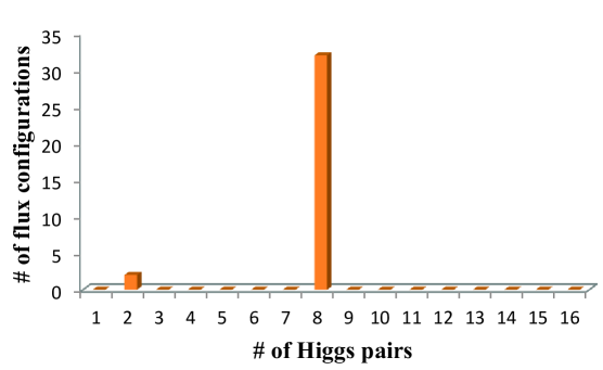
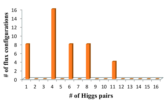
Figure 1: The number of magnetic flux configurations for each number of Higgs pairs in the type1 models where Higgs multiplets come from $\phi_{3}$. The upper panel corresponds to the case with $M^{(3)}={\rm diag}\,(0,1,-1)$ and the lower panel corresponds to $M^{(3)}={\rm diag}\,(0,1,0)$ or ${\rm diag}\,(0,0,-1)$ .

Next, in Fig. 2 we show the result about the type2 models where left-handed and right-handed matter fields have the opposite chirality on the first two tori. What is quite different from the type1 is that all the numbers of Higgs pairs up to 16 are allowed (at least in our searching region). One-pair Higgs models are also possible.

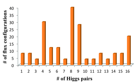
Figure 2: The number of magnetic fluxes for each number of Higgs pairs in the type2 models where Higgs multiplets come from the mixture of $\phi_{1}$ and $\phi_{2}$.

We find many possibilities to construct the models consistent with the MSSM and we obtain more various flavor structures. In particular, nonfactorizable fluxes enable us to construct one-pair Higgs models. We show the details of such typical models in the following.

4.3 One-pair Higgs models

Here, we focus on the models, which have a pair of Higgs doublets just like the MSSM. There are various flux configurations to give such models. Now, let us show details of a typical one included in the type1 models. The flux configuration is set as,

$$(M^{(1)}_{C},M^{(1)}_{L},M^{(1)}_{R})~{}~{} =(0,-2,-1),$$

$$(M^{(2)}_{C},M^{(2)}_{L},M^{(2)}_{R})~{}~{} =(0,+1,+2),$$

$$(M^{(3)}_{C},M^{(3)}_{L},M^{(3)}_{R})~{}~{} =(0,0,-1),$$

$$(M^{(12)}_{C},M^{(12)}_{L},M^{(12)}_{R}) =(0,+1,+1),$$

$$(M^{(21)}_{C},M^{(21)}_{L},M^{(21)}_{R}) =(0,+1,+1).$$

Then, the differences of fluxes which appear in zero-mode equations of multiplets are obtained as

$$\mathcal{M}_{L}=\left(\begin{array}[]{cc}+2&-1\\ -1&-1\end{array}\right),\qquad\mathcal{M}_{R}=\left(\begin{array}[]{cc}-1&+1\\ +1&+2\end{array}\right),\qquad\mathcal{M}_{H}=\left(\begin{array}[]{cc}-1&0\\ 0&-1\end{array}\right),$$

$$M^{(3)}_{C}-M^{(3)}_{L}=0,\quad\qquad M^{(3)}_{R}-M^{(3)}_{C}=-1,\quad\qquad M^{(3)}_{L}-M^{(3)}_{R}=+1,$$

where a subscript $L$ in $\mathcal{M}_{L}$ means left-handed matter fields, $R$ does right-handed matter and $H$ does Higgs fields. The absolute values of the determinants, $\mathcal{M}_{L}$ and $\mathcal{M}_{R}$, are equal to three and they originate three generation structures. In contrast, a determinant of $\mathcal{M}_{H}$ is equal to one, and fluxes on the third torus do not have any effects on the number of degenerate zero-modes. With these fluxes, we have the following zero-mode contents, block off-diagonal parts of $\phi_{1}$ and $\phi_{2}$, which are mixed up shown in Eq. (71):

$$\Phi^{{\cal I}_{ab}} =\left(\begin{array}[]{cc|c|cc}&&Q^{I}&0&0\\ &&L^{I}&0&0\\ \hline\cr 0&0&&0&0\\ \hline\cr U^{J}&N^{J}&0&&\\ D^{J}&E^{J}&0&&\end{array}\right),$$

block diagonal parts of $\phi_{1}$ and $\phi_{2}$, which do not feel the fluxes and each of zero modes exists separately:

$$\phi_{1}^{{\cal I}_{ab}} =\left(\begin{array}[]{cc|c|cc}\Omega_{C}^{(1)}&\Xi_{CC^{\prime}}^{(1)}&&&\\ \Xi_{C^{\prime}C}^{(1)}&\Omega_{C^{\prime}}^{(1)}&&&\\ \hline\cr&&\Omega_{L}^{(1)}&&\\ \hline\cr&&&\Omega_{R^{\prime}}^{(1)}&\Xi_{R^{\prime}R^{\prime\prime}}^{(1)}\\ &&&\Xi_{R^{\prime\prime}R^{\prime}}^{(1)}&\Omega_{R^{\prime\prime}}^{(1)}\end{array}\right),~{}~{}\phi_{2}^{{\cal I}_{ab}}=\left(\begin{array}[]{cc|c|cc}\Omega_{C}^{(2)}&\Xi_{CC^{\prime}}^{(2)}&&&\\ \Xi_{C^{\prime}C}^{(2)}&\Omega_{C^{\prime}}^{(2)}&&&\\ \hline\cr&&\Omega_{L}^{(2)}&&\\ \hline\cr&&&\Omega_{R^{\prime}}^{(2)}&\Xi_{R^{\prime}R^{\prime\prime}}^{(2)}\\ &&&\Xi_{R^{\prime\prime}R^{\prime}}^{(2)}&\Omega_{R^{\prime\prime}}^{(2)}\end{array}\right),$$

and the field $\phi_{3}$:

$$\phi_{3}^{{\cal I}_{ab}} =\left(\begin{array}[]{cc|c|cc}\Omega_{C}^{(3)}&\Xi_{CC^{\prime}}^{(3)}&0&0&0\\ \Xi_{C^{\prime}C}^{(3)}&\Omega_{C^{\prime}}^{(3)}&0&0&0\\ \hline\cr 0&0&\Omega_{L}^{(3)}&H_{u}&H_{d}\\ \hline\cr 0&0&0&\Omega_{R^{\prime}}^{(3)}&\Xi_{R^{\prime}R^{\prime\prime}}^{(3)}\\ 0&0&0&\Xi_{R^{\prime\prime}R^{\prime}}^{(3)}&\Omega_{R^{\prime\prime}}^{(3)}\end{array}\right),$$

where we use the same notations as we use in the previous section, however, Higgs doublets do not have a generation index. The three generation chiral matter fields and one pair of Higgs fields are realized just like the MSSM. Although all the chiral exotic fields are eliminated by the fluxes, there are some vector-like exotic modes and open string moduli. With all flux configurations which give one-pair Higgs type1 models, the same contents are generated.

We show the explicit form of Yukawa matrices of this model in Appendix B. According to that, Yukawa matrices can be full-rank and hierarchical, and all the elements of Yukawa matrices can take nonzero values different from each other. Thus, it would be possible to give a realistic pattern of quark and lepton masses and their mixings. We will study numerically these values elsewhere.

In Table 3 we show all the patterns of magnetic flux configurations, which give such one-pair Higgs models included in the type1. We choose $M_{C}=0$ and the first one (No. 1) corresponds to the above.

	$M_{L}^{(1)}$	$M_{R}^{(1)}$	$M_{L}^{(2)}$	$M_{R}^{(2)}$	$M_{L}^{(3)}$	$M_{R}^{(3)}$	$m_{L}^{(12)}$	$m_{R}^{(12)}$	$m_{L}^{(21)}$	$m_{R}^{(21)}$
No. 1	$-2$	$-1$	$+1$	$+2$	$0$	$-1$	$+1$	$+1$	$+1$	$+1$
No. 2	$-2$	$-1$	$+1$	$+2$	$+1$	$0$	$+1$	$+1$	$+1$	$+1$
No. 3	$+1$	$+2$	$-2$	$-1$	$0$	$-1$	$+1$	$+1$	$+1$	$+1$
No. 4	$+1$	$+2$	$-2$	$-1$	$+1$	$0$	$+1$	$+1$	$+1$	$+1$
No. 5	$-2$	$+3$	$+1$	$+2$	$0$	$-1$	$+1$	$+3$	$+1$	$+3$
No. 6	$+1$	$+2$	$-2$	$+3$	$0$	$-1$	$+1$	$+3$	$+1$	$+3$
No. 7	$-3$	$+2$	$-2$	$-1$	$+1$	$0$	$+3$	$+1$	$+3$	$+1$
No. 8	$-2$	$-1$	$-3$	$+2$	$+1$	$0$	$+3$	$+1$	$+3$	$+1$

Table 3: One-pair Higgs models in type1.

Next, we study the details of one-pair Higgs models included in the type2 models. We show one example of flux configurations as follows,

$$(M^{(1)}_{C},M^{(1)}_{L},M^{(1)}_{R})~{}~{} =(0,-1,-1)$$

$$(M^{(2)}_{C},M^{(2)}_{L},M^{(2)}_{R})~{}~{} =(0,+2,-7)$$

$$(M^{(3)}_{C},M^{(3)}_{L},M^{(3)}_{R})~{}~{} =(0,0,+1)$$

$$(M^{(12)}_{C},M^{(12)}_{L},M^{(12)}_{R}) =(0,-1,-2)$$

$$(M^{(21)}_{C},M^{(21)}_{L},M^{(21)}_{R}) =(0,-1,-2),$$

then

$$\mathcal{M}_{L}=\left(\begin{array}[]{cc}+1&+1\\ +1&-2\end{array}\right),\qquad\mathcal{M}_{R}=\left(\begin{array}[]{cc}-1&-2\\ -2&-7\end{array}\right),\qquad\mathcal{M}_{H}=\left(\begin{array}[]{cc}0&+1\\ +1&+9\end{array}\right),$$ (79)

$$M^{(3)}_{C}-M^{(3)}_{L}=0,\quad\qquad M^{(3)}_{L}-M^{(3)}_{R}=+1,\quad\qquad M^{(3)}_{R}-M^{(3)}_{C}=-1.$$

The zero-mode contents are as follows, block off-diagonal parts of $\phi_{1}$ and $\phi_{2}$, which are mixed up shown in Eq. (71):

$$\Phi^{{\cal I}_{ab}} =\left(\begin{array}[]{cc|c|cc}&&Q^{I}&0&0\\ &&L^{I}&0&0\\ \hline\cr 0&0&&H_{u}&H_{d}\\ \hline\cr 0&0&0&&\\ 0&0&0&&\end{array}\right),$$

block diagonal parts of $\phi_{1}$ and $\phi_{2}$, which do not feel the fluxes and each of zero modes exists separately:

$$\phi_{1}^{{\cal I}_{ab}} =\left(\begin{array}[]{cc|c|cc}\Omega_{C}^{(1)}&\Xi_{CC^{\prime}}^{(1)}&&&\\ \Xi_{C^{\prime}C}^{(1)}&\Omega_{C^{\prime}}^{(1)}&&&\\ \hline\cr&&\Omega_{L}^{(1)}&&\\ \hline\cr&&&\Omega_{R^{\prime}}^{(1)}&\Xi_{R^{\prime}R^{\prime\prime}}^{(1)}\\ &&&\Xi_{R^{\prime\prime}R^{\prime}}^{(1)}&\Omega_{R^{\prime\prime}}^{(1)}\end{array}\right),~{}~{}\phi_{2}^{{\cal I}_{ab}}=\left(\begin{array}[]{cc|c|cc}\Omega_{C}^{(2)}&\Xi_{CC^{\prime}}^{(2)}&&&\\ \Xi_{C^{\prime}C}^{(2)}&\Omega_{C^{\prime}}^{(2)}&&&\\ \hline\cr&&\Omega_{L}^{(2)}&&\\ \hline\cr&&&\Omega_{R^{\prime}}^{(2)}&\Xi_{R^{\prime}R^{\prime\prime}}^{(2)}\\ &&&\Xi_{R^{\prime\prime}R^{\prime}}^{(2)}&\Omega_{R^{\prime\prime}}^{(2)}\end{array}\right),$$

and the field $\phi_{3}$:

$$\phi_{3}^{{\cal I}_{ab}} =\left(\begin{array}[]{cc|c|cc}\Omega_{C}^{(3)}&\Xi_{CC^{\prime}}^{(3)}&0&0&0\\ \Xi_{C^{\prime}C}^{(3)}&\Omega_{C^{\prime}}^{(3)}&0&0&0\\ \hline\cr 0&0&\Omega_{L}^{(3)}&0&0\\ \hline\cr U^{J}&N^{J}&0&\Omega_{R^{\prime}}^{(3)}&\Xi_{R^{\prime}R^{\prime\prime}}^{(3)}\\ D^{J}&E^{J}&0&\Xi_{R^{\prime\prime}R^{\prime}}^{(3)}&\Omega_{R^{\prime\prime}}^{(3)}\end{array}\right).$$

In this model, zero-mode contents are the same as the previous ones in type1. Furthermore, Yukawa matrices can be full-rank and hierarchical, and all the elements of Yukawa matrices can take non-zero values different from each other.

There are eight flux configurations which give one-pair Higgs models included in the type2 model, and these are shown in Table 4. The first one, No. 1, in Table 4 corresponds to the above. The four patterns from No. 1 to No. 4 give the same zero-mode contents. However, the zero-modes of the last four models, No. 5-8, include additional fields. In these models, the Higgs sector does not feel the nonfactorizable fluxes ($m^{(ij)}_{L}-m^{(ij)}_{R}=0$ ) and we get their zero-modes separately in $\phi_{1}$ and $\phi_{2}$. Furthermore, the factorizable fluxes on the third torus $M^{(3)}$ have no effect on the Higgs sector. That is the significant difference from models, No. 1-4 in Table 3. Then, the models have the MSSM Higgs correctly in $\phi_{1}$ and also have representations conjugate to the Higgs pair but can not couple with quarks and leptons in $\phi_{2}$.

	$M_{L}^{(1)}$	$M_{R}^{(1)}$	$M_{L}^{(2)}$	$M_{R}^{(2)}$	$M_{L}^{(3)}$	$M_{R}^{(3)}$	$m_{L}^{(12)}$	$m_{R}^{(12)}$	$m_{L}^{(21)}$	$m_{R}^{(21)}$
No. 1	$-1$	$-1$	$+2$	$-7$	$0$	$+1$	$-1$	$-2$	$-1$	$-2$
No. 2	$2$	$-7$	$-1$	$-1$	$0$	$+1$	$-1$	$-2$	$-1$	$-2$
No. 3	$-1$	$-4$	$+2$	$-3$	$0$	$+1$	$+1$	$-3$	$+1$	$-3$
No. 4	$2$	$-3$	$-1$	$-4$	$0$	$+1$	$+1$	$-3$	$+1$	$-3$
No. 5	$-2$	$-3$	$-9$	$-8$	$+1$	$+1$	$+3$	$+3$	$+7$	$+7$
No. 6	$-2$	$-3$	$-9$	$-8$	$+1$	$+1$	$+7$	$+7$	$+3$	$+3$
No. 7	$-2$	$-3$	$-9$	$-8$	$+1$	$+1$	$-3$	$-3$	$-7$	$-7$
No. 8	$-2$	$-3$	$-9$	$-8$	$+1$	$+1$	$-7$	$-7$	$-3$	$-3$

Table 4: One-pair Higgs models in type2.

4.4 Nonfactorizable flux models on $T^{6}/Z_{2}$ orbifolds

There are other possibilities for model building. We can consider nonfactorizable fluxes with orbifold projection, where magnetic fluxes have to be five-block forms because (continuous) Wilson lines cannot be introduced to break the gauge group by the orbifold projection. When we consider the $Z_{2}$ projection Eq. (51) either even or odd modes of zero-modes remain. How to derive even and odd functions from Eq. (12) and (13) has already known for factorizable fluxes in Ref.[15], and we find that even and odd functions can be derived from Eq. (69) and (70) as natural generalization of the factorizable case Eq. (50) as,

$$\phi_{\mathrm{even}}^{\vec{j}}(\vec{z})=\frac{1}{\sqrt{2}}(\phi^{\vec{j},{\mathcal{M}}}(\vec{z})+\phi^{\vec{e}-\vec{j},{\mathcal{M}}}(\vec{z})),$$

$$\phi_{\mathrm{odd}}^{\vec{j}}(\vec{z})=\frac{1}{\sqrt{2}}(\phi^{\vec{j},{\mathcal{M}}}(\vec{z})-\phi^{\vec{e}-\vec{j},{\mathcal{M}}}(\vec{z})),$$

where,

$$\vec{e}\equiv\vec{e}_{1}+\vec{e}_{2}=\begin{pmatrix}1\\ 0\end{pmatrix}+\begin{pmatrix}0\\ 1\end{pmatrix}=\begin{pmatrix}1\\ 1\end{pmatrix}.$$

Note that we use the following relations to obtain these functions,

$$\phi^{\vec{j},{\mathcal{M}}}(-\vec{z}\hskip 1.0pt)=\phi^{\vec{e}-\vec{j},{\mathcal{M}}}(\vec{z}\hskip 1.0pt).$$

According to that, we find that a rule for the number of the degenerate zero-modes after a $Z_{2}$ projection is the same as factorizable cases and we see the rule in Table 2 with replacing $M$ by $\det\mathcal{M}$.

On such a background, we search flux configurations to give the three generation models in a systematic way and the range between $-10$ and 10. As a result, we could not construct three generation models with four-block or five-block fluxes because SUSY conditions are severe.

5 Conclusions and discussions

We have carried out a systematic search for possibilities to construct models in which we obtain preserved $\mathcal{N}=1$ SUSY, the SM gauge group, all the MSSM fields, three generation structures of quarks and leptons and full-rank Yukawa matrices.

First, we have done that considering only the factorizable fluxes, then we find that the Pati-Salam models with six pairs of Higgs multiplets can be constructed.

An orbifold projection could eliminate exotic modes without changing three generation structures of quarks and leptons. It also can change the number of degenerate zero-modes if $Z_{2}$ act on the torus where flavor structures are generated, and we try to use that to generate three generation structures other than previous ones. With such an orbifold projection, (continuous) Wilson lines are not allowed and we have to break the gauge group using only magnetic fluxes. Thus, we have to consider five-block magnetic fluxes for which SUSY conditions become more severe and we find it impossible.

We can consider nonfactorizable fluxes which cross over two tori. Considering nonfactorizable fluxes, more various model buildings become possible. With such fluxes we tried to construct the Pati-Salam models, and we find that there are infinite possibilities to give three generation models as a result of systematic research. We also find some particular values are allowed for the number of Higgs pairs if Higgs multiplets come from $\phi_{3}$, in contrast any numbers of Higgs pairs can be realized in the other case. Furthermore, the quite attractive fact is that we can construct one-pair Higgs models just like the MSSM. Finally, we tried to construct nonfactorizable flux models on $T^{6}/Z_{2}$ orbifolds. As a result we cannot find a flux configuration to give us the plausible model.

In this paper we have found many possibilities to give the plausible models, which have the three generation quark and lepton multiplets and full-rank Yukawa matrices, other than the one studied in Ref. [11]. Plausible flux configurations give only the Pati-Salam models, where we need introduce Wilson lines to break the gauge group. In the Pati-Salam models with only factorizable fluxes, Yukawa coupling possesses the flavor symmetry $\Delta(27)$[6]. It is interesting to study how such structures would be changed by nonfactorizable fluxes. Furthermore, introducing nonfactorizable fluxes has a close connection with the moduli stabilization. We will study these feature of nonfactorizable fluxes elsewhere.

The five-block flux models not needing Wilson lines cannot be realized in 10D magnetized SYM theory. However, it would be straightforward to extend our study to SYM theories in a lower than ten-dimensional spacetime, or even to the mixture of SYM theories with a different dimensionality. For example, in type IIB orientifolds, our study will be adopted not only to the magnetized D9 branes, which are T-dual to intersecting D6 branes in the IIA side, but also to the D5-D9 [22] and the D3-D7 brane configurations with magnetic fluxes in the extra dimensions. With such brane configurations, we might be able to build the five-block and more various models.

As other generalizations, we can consider generalized torus in which off-diagonal elements of general complex structure $\Omega$ have nonzero values, or more complicated manifold, and that would give us a new flavor landscape.

Finally, our models derived from supersymmetric Yang-Mills theory might be embedded in the matrix models [24]. In that case, it would give us a new motivation to study the magnetized supersymmetric Yang-Mills theory.

Acknowledgement

H.A. was supported in part by the Grant-in-Aid for Scientific Research No. 25800158 from the Ministry of Education, Culture, Sports, Science and Technology (MEXT) in Japan. T.K. was supported in part by the Grant-in-Aid for Scientific Research No. 25400252 from the MEXT in Japan. H.O. was supported in part by the JSPS Grant-in-Aid for Scientific Research (S) No. 22224003, for young Scientists (B) No. 25800139 from the MEXT in Japan. K.S. was supported in part by a Grant-in-Aid for JSPS Fellows No. 25$\cdot$4968 and a Grant for Excellent Graduate Schools from the MEXT in Japan. Y.T. was supported in part by a Grant for Excellent Graduate Schools from the MEXT in Japan. Y.T. would like to thank T. Shoji and K. Oh for a correspondence.

Appendix A Exotic modes with the pattern1 fluxes

For the matter profile (48) caused by the type1 magnetic fluxes in Table. 1, we see that $Z_{2}$-projection introduced in Sec. 3 which acts on the second and the third tori with the following projection operator,

$$P_{ab} = \left(\begin{array}[]{ccc}-{\bm{1}}_{4}&0&0\\ 0&+{\bm{1}}_{2}&0\\ 0&0&+{\bm{1}}_{2}\end{array}\right),$$ (83)

removes most of the massless exotic modes $\Xi_{ab}^{(r)}$ and some of massless diagonal components $\Omega_{a}^{(r)}$. The matter contents on the orbifold $T^{6}/Z_{2}$ are found as

$$\phi_{1}^{{\cal I}_{ab}} = \left(\begin{array}[]{cc|c|cc}\Omega_{C}^{(1)}&\Xi_{CC^{\prime}}^{(1)}&0&0&0\\ \Xi_{C^{\prime}C}^{(1)}&\Omega_{C^{\prime}}^{(1)}&0&0&0\\ \hline\cr 0&0&\Omega_{L}^{(1)}&H_{u}^{K}&H_{d}^{K}\\ \hline\cr 0&0&0&\Omega_{R^{\prime}}^{(1)}&\Xi_{R^{\prime}R^{\prime\prime}}^{(1)}\\ 0&0&0&\Xi_{R^{\prime\prime}R^{\prime}}^{(1)}&\Omega_{R^{\prime\prime}}^{(1)}\end{array}\right),$$ (89)

$$\phi_{2}^{{\cal I}_{ab}} = \left(\begin{array}[]{cc|c|cc}0&0&Q^{I}&0&0\\ 0&0&L^{I}&0&0\\ \hline\cr 0&0&0&0&0\\ \hline\cr 0&0&0&0&0\\ 0&0&0&0&0\end{array}\right),\qquad\phi_{3}^{{\cal I}_{ab}}\ =\ \left(\begin{array}[]{cc|c|cc}0&0&0&0&0\\ 0&0&0&0&0\\ \hline\cr 0&0&0&0&0\\ \hline\cr U^{J}&N^{J}&0&0&0\\ D^{J}&E^{J}&0&0&0\end{array}\right),$$ (100)

where $I,J=1,2,3$ and $K=1,\ldots,6$ label the generations as before. There still remain massless exotic modes $\Xi_{ab}^{(1)}$ for $a,b=C,C^{\prime}$ and $a,b=R^{\prime},R^{\prime\prime}$ with $a\neq b$ as well as open string moduli $\Omega_{a}^{(1)}$ for $a=C,C^{\prime},L,R^{\prime},R^{\prime\prime}$. That is one of the open problems in the $T^{6}/Z_{2}$ magnetized orbifold model. In Ref. [11], these exotic modes are assumed to become massive through some nonperturbative effects [23] or higher-order corrections, so that they decouple from the low-energy physics.

Appendix B Yukawa matrices in a one-pair Higgs model

We show an explicit form of Yukawa matrices in a one-pair Higgs model. Yukawa couplings of No.1 model in type1 are written by

$$Y_{ijk}\propto\sum_{\vec{m}}\delta_{\vec{k},\mathcal{M}_{H}^{-1}(\mathcal{M}_{L}\vec{i}+\mathcal{M}_{R}\vec{j}+\mathcal{M}_{L}\vec{m})}\int d^{2}y\left[e^{-\pi\vec{y}(\mathcal{M}_{L}\tilde{\Omega}_{L}+\mathcal{M}_{R}\tilde{\Omega}_{R}+\mathcal{M}_{H}\Omega)\cdot\vec{y}}\cdot\vartheta\begin{bmatrix}\vec{\mathbb{K}}\\[5.0pt] 0\end{bmatrix}(i\vec{\mathbb{Y}}|i\vec{\mathbb{Q}})\right]$$

where

$$\tilde{\Omega}_{L}=\hat{\Omega}_{L}\cdot\Omega,\qquad\tilde{\Omega}_{R}=\hat{\Omega}_{R}\cdot\Omega$$

$$\vec{\mathbb{K}}\equiv\left(\begin{array}[]{c}\vec{k}\\ (\vec{i}-\vec{j}+\vec{m})\frac{\mathcal{M}_{L}(\mathcal{M}_{L}+\mathcal{M}_{R})^{-1}\mathcal{M}_{R}}{\det\mathcal{M}_{L}\det\mathcal{M}_{R}}\end{array}\right)$$

$$\vec{\mathbb{Y}}\equiv\left(\begin{array}[]{c}(\mathcal{M}_{L}\tilde{\Omega}_{L}+\mathcal{M}_{R}\tilde{\Omega}_{R}+\mathcal{M}_{H}\Omega)\cdot\vec{y}\\ (\det\mathcal{M}_{L}\det\mathcal{M}_{R})(\mathcal{M}_{L}\tilde{\Omega}_{L}(\mathcal{M}_{L}^{-1})^{T}-\mathcal{M}_{R}\tilde{\Omega}_{R}(\mathcal{M}_{R}^{-1})^{T})\cdot\vec{y})\end{array}\right)$$

$$\vec{\mathbb{Q}}\equiv\left(\begin{array}[]{cc}\mathcal{M}_{L}\tilde{\Omega}_{L}+\mathcal{M}_{R}\tilde{\Omega}_{R}+\mathcal{M}_{H}\Omega&(\det\mathcal{M}_{L}\det\mathcal{M}_{R})(\mathcal{M}_{L}\tilde{\Omega}_{L}\cdot(\mathcal{M}_{L}^{-1})^{T}-\mathcal{M}_{R}\tilde{\Omega}_{R}\cdot(\mathcal{M}_{R}^{-1})^{T})\\ (\det\mathcal{M}_{L}\det\mathcal{M}_{R})(\tilde{\Omega}_{L}-\tilde{\Omega}_{R})&(\det\mathcal{M}_{L}\det\mathcal{M}_{R})^{2}(\tilde{\Omega}_{L}\mathcal{M}_{L}^{-1}+\tilde{\Omega}_{R}\mathcal{M}_{R}^{-1})\end{array}\right).$$

We define

$$\eta\left[(\vec{i}-\vec{j}+\vec{m})\frac{\mathcal{M}_{L}(\mathcal{M}_{L}+\mathcal{M}_{R})^{-1}\mathcal{M}_{R}}{\det\mathcal{M}_{L}\det\mathcal{M}_{R}}\right]\equiv\vartheta\begin{bmatrix}\vec{\mathbb{K}}\\[5.0pt] 0\end{bmatrix}(i\vec{\mathbb{Y}}|i\vec{\mathbb{Q}}),$$

and then $(1,1)$ element can be written using $\eta$;

$$\lambda_{11}=\eta[(0,0)]+\eta[(0,\tfrac{1}{3})]+\eta[(0,\tfrac{2}{3})]+\eta[(\tfrac{1}{3},0)]+\eta[(\tfrac{1}{3},\tfrac{1}{3})]+\eta[(\tfrac{1}{3},\tfrac{2}{3})]+\eta[(\tfrac{2}{3},0)]+\eta[(\tfrac{2}{3},\tfrac{1}{3})]+\eta[(\tfrac{2}{3},\tfrac{2}{3})].$$

Similarly, other elements are written by

$$\lambda_{12} =\eta[(\tfrac{1}{9},\tfrac{1}{9})]+\eta[(\tfrac{1}{9},\tfrac{4}{9})]+\eta[(\tfrac{1}{9},\tfrac{7}{9})]+\eta[(\tfrac{4}{9},\tfrac{1}{9})]+\eta[(\tfrac{4}{9},\tfrac{4}{9})]+\eta[(\tfrac{4}{9},\tfrac{7}{9})]+\eta[(\tfrac{7}{9},\tfrac{1}{9})]+\eta[(\tfrac{7}{9},\tfrac{4}{9})]+\eta[(\tfrac{7}{9},\tfrac{7}{9})]$$

$$\lambda_{13} =\eta[(\tfrac{2}{9},\tfrac{2}{9})]+\eta[(\tfrac{2}{9},\tfrac{5}{9})]+\eta[(\tfrac{2}{9},\tfrac{8}{9})]+\eta[(\tfrac{5}{9},\tfrac{2}{9})]+\eta[(\tfrac{5}{9},\tfrac{5}{9})]+\eta[(\tfrac{5}{9},\tfrac{8}{9})]+\eta[(\tfrac{8}{9},\tfrac{2}{9})]+\eta[(\tfrac{8}{9},\tfrac{5}{9})]+\eta[(\tfrac{8}{9},\tfrac{8}{9})]$$

$$\lambda_{21} =\eta[(\tfrac{2}{9},\tfrac{1}{9})]+\eta[(\tfrac{2}{9},\tfrac{4}{9})]+\eta[(\tfrac{2}{9},\tfrac{7}{9})]+\eta[(\tfrac{5}{9},\tfrac{1}{9})]+\eta[(\tfrac{5}{9},\tfrac{4}{9})]+\eta[(\tfrac{5}{9},\tfrac{7}{9})]+\eta[(\tfrac{8}{9},\tfrac{1}{9})]+\eta[(\tfrac{8}{9},\tfrac{4}{9})]+\eta[(\tfrac{8}{9},\tfrac{7}{9})]$$

$$\lambda_{22} =\eta[(0,\tfrac{2}{9})]+\eta[(0,\tfrac{5}{9})]+\eta[(0,\tfrac{8}{9})]+\eta[(\tfrac{1}{3},\tfrac{2}{9})]+\eta[(\tfrac{1}{3},\tfrac{5}{9})]+\eta[(\tfrac{1}{3},\tfrac{8}{9})]+\eta[(\tfrac{2}{3},\tfrac{2}{9})]+\eta[(\tfrac{2}{3},\tfrac{5}{9})]+\eta[(\tfrac{2}{3},\tfrac{8}{9})]$$

$$\lambda_{23} =\eta[(\tfrac{1}{9},0)]+\eta[(\tfrac{1}{9},\tfrac{1}{3})]+\eta[(\tfrac{1}{9},\tfrac{2}{3})]+\eta[(\tfrac{4}{9},0)]+\eta[(\tfrac{4}{9},\tfrac{1}{3})]+\eta[(\tfrac{4}{9},\tfrac{2}{3})]+\eta[(\tfrac{7}{9},0)]+\eta[(\tfrac{7}{9},\tfrac{1}{3})]+\eta[(\tfrac{7}{9},\tfrac{2}{3})]$$

$$\lambda_{31} =\eta[(\tfrac{1}{9},\tfrac{2}{9})]+\eta[(\tfrac{1}{9},\tfrac{5}{9})]+\eta[(\tfrac{1}{9},\tfrac{8}{9})]+\eta[(\tfrac{4}{9},\tfrac{2}{9})]+\eta[(\tfrac{4}{9},\tfrac{5}{9})]+\eta[(\tfrac{4}{9},\tfrac{8}{9})]+\eta[(\tfrac{7}{9},\tfrac{2}{9})]+\eta[(\tfrac{7}{9},\tfrac{5}{9})]+\eta[(\tfrac{7}{9},\tfrac{8}{9})]$$

$$\lambda_{32} =\eta[(\tfrac{2}{9},0)]+\eta[(\tfrac{2}{9},\tfrac{1}{3})]+\eta[(\tfrac{2}{9},\tfrac{2}{3})]+\eta[(\tfrac{5}{9},0)]+\eta[(\tfrac{5}{9},\tfrac{1}{3})]+\eta[(\tfrac{5}{9},\tfrac{2}{3})]+\eta[(\tfrac{7}{9},0)]+\eta[(\tfrac{7}{9},\tfrac{1}{3})]+\eta[(\tfrac{7}{9},\tfrac{2}{3})]$$

$$\lambda_{33} =\eta[(0,\tfrac{1}{9})]+\eta[(0,\tfrac{4}{9})]+\eta[(0,\tfrac{7}{9})]+\eta[(\tfrac{1}{3},\tfrac{1}{9})]+\eta[(\tfrac{1}{3},\tfrac{4}{9})]+\eta[(\tfrac{1}{3},\tfrac{7}{9})]+\eta[(\tfrac{2}{3},\tfrac{1}{9})]+\eta[(\tfrac{2}{3},\tfrac{4}{9})]+\eta[(\tfrac{2}{3},\tfrac{7}{9})],$$

and total Yukawa matrices can be written as follows

$$Y_{ijk}\propto\int d^{2}y\left[e^{-\pi\vec{y}(\mathcal{M}_{L}\tilde{\Omega}_{L}+\mathcal{M}_{R}\tilde{\Omega}_{R}+\mathcal{M}_{H}\Omega)\vec{y}}\left(\begin{array}[]{ccc}\lambda_{11}&\lambda_{12}&\lambda_{13}\\ \lambda_{21}&\lambda_{22}&\lambda_{23}\\ \lambda_{31}&\lambda_{32}&\lambda_{33}\end{array}\right)\right].$$

The values of elements are different from each other, and we cannot find any non-Abelian flavor symmetry there.

References

• [1] L. E. Ibanez and A. M. Uranga, “String theory and particle physics: An introduction to string phenomenology,” Cambridge, UK: Univ. Pr. (2012) 673 p.
• [2] C. Bachas, arXiv:hep-th/9503030; R. Blumenhagen, L. Goerlich, B. Kors and D. Lust, JHEP 0010, 006 (2000) [arXiv:hep-th/0007024]; C. Angelantonj, I. Antoniadis, E. Dudas and A. Sagnotti, Phys. Lett.  B 489, 223 (2000) [arXiv:hep-th/0007090]; R. Blumenhagen, B. Kors and D. Lust, JHEP 0102, 030 (2001) [arXiv:hep-th/0012156].
• [3] D. Cremades, L. E. Ibanez and F. Marchesano, JHEP 0405 (2004) 079 [hep-th/0404229].
• [4] H. Abe, K. -S. Choi, T. Kobayashi and H. Ohki, Nucl. Phys. B 814 (2009) 265 [arXiv:0812.3534 [hep-th]].
• [5] H. Abe, K. -S. Choi, T. Kobayashi and H. Ohki, JHEP 0906, 080 (2009) [arXiv:0903.3800 [hep-th]].
• [6] H. Abe, K. -S. Choi, T. Kobayashi and H. Ohki, Nucl. Phys. B 820 (2009) 317 [arXiv:0904.2631 [hep-ph]].
• [7] H. Abe, K. -S. Choi, T. Kobayashi and H. Ohki, Phys. Rev. D 80 (2009) 126006 [arXiv:0907.5274 [hep-th]]; Phys. Rev. D 81 (2010) 126003 [arXiv:1001.1788 [hep-th]].
• [8] M. Berasaluce-Gonzalez, P. G. Camara, F. Marchesano, D. Regalado and A. M. Uranga, JHEP 1209, 059 (2012) [arXiv:1206.2383 [hep-th]].
• [9] F. Marchesano, D. Regalado and L. Vázquez-Mercado, arXiv:1306.1284 [hep-th].
• [10] H. Abe, T. Kobayashi, H. Ohki and K. Sumita, Nucl. Phys. B 863 (2012) 1 [arXiv:1204.5327 [hep-th]].
• [11] H. Abe, T. Kobayashi, H. Ohki, A. Oikawa and K. Sumita, Nucl. Phys. B 870 (2013) 30 [arXiv:1211.4317 [hep-ph]].
• [12] I. Antoniadis, A. Kumar and B. Panda, Nucl. Phys. B 823 (2009) 116 [arXiv:0904.0910 [hep-th]].
• [13] L. De Angelis, R. Marotta, F. Pezzella and R. Troise, JHEP 1210 (2012) 052 [arXiv:1206.3401 [hep-th]].
• [14] M. Sakamoto and S. Tanimura, J. Math. Phys.  44, 5042 (2003) [hep-th/0306006].
• [15] H. Abe, T. Kobayashi and H. Ohki, JHEP 0809 (2008) 043 [arXiv:0806.4748 [hep-th]].
• [16] S. Groot Nibbelink and P. K. S. Vaudrevange, JHEP 1303, 142 (2013) [arXiv:1212.4033 [hep-th]].
• [17] Y. Fujimoto, T. Kobayashi, T. Miura, K. Nishiwaki and M. Sakamoto, arXiv:1302.5768 [hep-th].
• [18] N. Marcus, A. Sagnotti and W. Siegel, Nucl. Phys. B 224 (1983) 159; N. Arkani-Hamed, T. Gregoire and J. G. Wacker, JHEP 0203 (2002) 055 [hep-th/0101233].
• [19] K. -S. Choi, T. Kobayashi, R. Maruyama, M. Murata, Y. Nakai, H. Ohki and M. Sakai, Eur. Phys. J. C 67, 273 (2010) [arXiv:0908.0395 [hep-ph]]. T. Kobayashi, R. Maruyama, M. Murata, H. Ohki and M. Sakai, JHEP 1005, 050 (2010) [arXiv:1002.2828 [hep-ph]].
• [20] Y. Hamada and T. Kobayashi, Prog. Theor. Phys.  128, 903 (2012) [arXiv:1207.6867 [hep-th]].
• [21] H. M. Lee, H. P. Nilles and M. Zucker, Nucl. Phys. B 680 (2004) 177 [hep-th/0309195].
• [22] P. Di Vecchia, R. Marotta, I. Pesando and F. Pezzella, J. Phys. A A 44 (2011) 245401 [arXiv:1101.0120 [hep-th]].
• [23] L. E. Ibanez and A. M. Uranga, JHEP 0703 (2007) 052 [hep-th/0609213]; M. Cvetic, R. Richter and T. Weigand, Phys. Rev. D 76 (2007) 086002 [hep-th/0703028].
• [24] J. Nishimura and A. Tsuchiya, arXiv:1305.5547 [hep-th]; H. Aoki, matrix model compactified on a torus,” arXiv:1303.3982 [hep-th].