Computing the Fréchet distance with shortcuts is NP-hard

Abstract

We study the shortcut Fréchet distance, a natural variant of the Fréchet distance, that allows us to take shortcuts from and to any point along one of the curves. The classic Fréchet distance is a bottle-neck distance measure and hence quite sensitive to outliers. The shortcut Fréchet distance allows us to cut across outliers and hence produces more meaningful results when dealing with real world data. Driemel and Har-Peled recently described approximation algorithms for the restricted case where shortcuts have to start and end at input vertices. We show that, in the general case, the problem of computing the shortcut Fréchet distance is NP-hard. This is the first hardness result for a variant of the Fréchet distance between two polygonal curves in the plane. We also present two algorithms for the decision problem: a $3$-approximation algorithm for the general case and an exact algorithm for the vertex-restricted case. Both algorithms run in $O(n^{3}\log n)$ time.

1 Introduction

Measuring the similarity of two curves is an important problem which occurs in many applications. A popular distance measure, that takes into account the continuity of the curves, is the Fréchet distance. Imagine walking forwards along both of the two curves whose similarity is to be measured. At any point in time, the positions on the two curves have to stay within distance ${\varepsilon}$. The minimal ${\varepsilon}$ for which such a traversal is possible is the Fréchet distance. It has been used for simplification [1, 4], clustering [7], and map-matching [2, 13]. The Fréchet distance also has applications in matching biological sequences [16], analysing tracking data [5, 6], and matching coastline data [15].

Despite its versatility, the Fréchet distance has one serious drawback: it is a bottleneck distance. Hence it is quite sensitive to outliers, which are frequent in real world data sets. To remedy this Driemel and Har-Peled [12] introduced a variant of the Fréchet distance, namely the shortcut Fréchet distance, that allows shortcuts from and to any point along one of the curves. The shortcut Fréchet distance is then defined as the minimal Fréchet distance over all possible such shortcut curves.

The shortcut Fréchet distance automatically cuts across outliers and allows us to ignore data specific “detours” in one of the curves. Hence it produces more meaningful results when dealing with real world data than the classic Fréchet distance. Consider the following two examples. Birds are known to use coastlines for navigation, e.g., the Atlantic flyway for migration. However, when the coastline takes a “detour”, like a harbor or the mouth of a river, the bird ignores this detour, and instead follows a “shortcut” across. See the example of a seagull in the figure, navigating along the coastline of Zeeland. Using the shortcut Fréchet distance, we can detect this similarity. Now imagine a hiker following a pilgrims route. The hiker will occasionally detour from the route, for breaks along the way. In the former example, shortcuts are allowed on the coastline, in the latter on the hiker’s path.

Related work

The standard Fréchet distance can be computed in time roughly quadratic in the complexity of the input curves [3, 8]. Driemel and Har-Peled introduce the notion of the shortcut Fréchet distance and describe approximation algorithms in the restricted case where shortcuts have to start and end at input vertices [12]. In particular, they give a $(3+{\varepsilon})$-approximation algorithm for the vertex-restricted shortcut Fréchet distance that runs in $O(n\log^{3}n)$ time under certain input assumptions. Specifically, they assume $c$-packedness, that is, the length of the input curves in any ball is at most $c$ times the radius of the ball, where $c$ is a constant. Their algorithm also yields a polynomial-time exact algorithm to compute the vertex-restricted shortcut Fréchet distance that runs in $O(n^{5}\log n)$ time and uses $O(n^{4})$ space without using any input assumptions [11].

The shortcut Fréchet distance can be interpreted as a partial distance measure, that is, it maps parts of one curve to another curve. In contrast to other partial distance measures, it is parameter-free. A different notion of a partial Fréchet distance was developed by Buchin et al. [9]. They propose the total length of the longest subcurves which lie within a given Fréchet distance to each other as similarity measure. The parts omitted are completely ignored, while in our definition these parts are substituted by shortcuts, which have to be matched under the Fréchet distance.

Results and Organization

We study the complexity of computing the shortcut Fréchet distance. Specifically, we show that in the general case, where shortcuts can be taken at any point along a curve, the problem of computing the shortcut Fréchet distance exactly is NP-hard. This is the first hardness result for a variant of the Fréchet distance between two polygonal curves in the plane.

Below we give an exact definition of the problem we study. In Section 2 we describe a reduction from SUBSET-SUM to the decision version of the shortcut Fréchet distance and in Section 3 we prove its correctness. The NP-hardness stems from an exponential number of combinatorially different shortcut curves which cause an exponential number of reachable components in the free space diagram. We use this in our reduction together with a mechanism that controls the sequence of free space components that may be visited.

In Section 4 we discuss polynomial-time solutions for approximation. We give two algorithms for the decision version of the problem, which both run in $O(n^{3}\log n)$ time. The decision algorithms traverse the free space (as usual for Fréchet distance algorithms), and make use of a line stabbing algorithm of Guibas et al. [14] to test whether shortcuts are admissible. The first algorithm uses a crucial lemma of Driemel and Har-Peled [12] to approximate the reachable free space and so prevents it from being fragmented. This yields a $3$-approximation algorithm for the decision version of the general shortcut Fréchet distance. The second algorithm concerns the vertex-restricted case. Here, the free space naturally does not fragment, however, the line-stabbing algorithm helps us to improve upon the running time of the exact decision algorithm described by Driemel [11]. We conclude with an extensive discussion of open problems in Section 5. In particular we discuss some challenges in extending the decision algorithm to the computation problem.

Definitions

A curve $T$ is a continuous mapping from $[0,1]$ to ${\rm I\!R}^{2}$, where $T(t)$ denotes the point on the curve parameterized by $t\in[0,1]$. Given two curves $T$ and $B$ in ${\rm I\!R}^{2}$, the Fréchet distance between them is

$$\mathsf{d}_{\mathcal{F}}\!\left({T,B}\right)=\inf_{\begin{subarray}{c}f:[0,1]\rightarrow[0,1]\end{subarray}}~{}\max_{\alpha\in[0,1]}\left\|{T(f(\alpha))-B(\alpha)}\right\|,$$

where $f$ is an orientation-preserving homeomorphism. We call the line segment between two arbitrary points $B(y)$ and $B(y^{\prime})$ on $B$ a shortcut on $B$. Replacing a number of subcurves of $B$ by the shortcuts connecting their endpoints results in a shortcut curve of $B$. Thus, a shortcut curve is an order-preserving concatenation of non-overlapping subcurves of $B$ that has straight line segments connecting the endpoints of the subcurves.

Our input are two polygonal curves: the target curve $T$ and base curve $B$. The shortcut Fréchet distance $\mathsf{d}_{\mathcal{S}}\!\left({T,B}\right)$ is now defined as the minimal Fréchet distance between the target curve $T$ and any shortcut curve of the base curve $B$.

2 NP-hardness reduction

We prove that deciding if the shortcut Fréchet distance between two given curves is smaller or equal a given value is weakly NP-hard by a reduction from SUBSET-SUM. We first discuss the main ideas and challenges in Section 2.1, then we formally describe the reduction in Section 2.2. The correctness is proven in Section 3.

2.1 General idea

The SUBSET-SUM instance is given as a set of input values and a designated sum value. A solution to the instance is a subset of these values that has the specified sum. We describe how to construct a target curve $T$ and a base curve $B$, such that there exists a shortcut curve of $B$ which is in Fréchet distance $1$ to $T$ if and only if there exists a solution to the SUBSET-SUM instance. We call such a shortcut curve feasible if it lies within Fréchet distance $1$. The construction of the curves is split into gadgets, each of them encoding one of the input values.

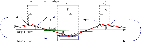
Figure 1: Simplistic version of the gadget encoding one of the input values $s_{i}$. A shortcut curve entering from a position on the edge $\mathsf{e}^{i-1}_{*}$ has the choice to visit either $\mathsf{e}^{i}$ or $\overline{\mathsf{e}}^{i}$. Its distance on $\mathsf{e}^{i}_{*}$ to the shortcut curve encoding the empty set ($x$ in the figure) is altered by $s_{i}$. The target curve is distorted to show its topology.

The idea of the reduction is as follows. We construct the target curve to lie on a horizontal line going mostly rightwards. The base curve has several horizontal edges which lie at distance exactly $1$ to the target curve and which go leftwards. We call these edges “mirrors” for reasons that will become clear later. All other edges of the base curve lie at distance greater than $1$ to the target curve. If a shortcut curve is feasible, then any of its shortcuts must start where the previous shortcut ended. This way, the shortcut curve “jumps” rightwards along the mirrors of the base curve and visits each edge in exactly one point. We restrict the solution space of feasible shortcut curves further by letting the target curve go leftwards for a distance $2$ and then rightwards again (see Figure 1). We call this a “twist”. We place the mirrors far enough from any twist, such that any shortcut curve which is feasible has to go through the center of each such twist, since it has to traverse the twist region using a shortcut and this shortcut has to have Fréchet distance at most $1$ to the twisting portion.

The reader may picture the shortcut curve as a lightbeam, which is reflected in all directions when it hits a mirror. In this analogy, the target curve is a wall which has a hole at the center of each twist, thus, these are the only points where light can go through. Only if we can send light from the first vertex of the base curve to the last vertex of the base curve, there exists a feasible shortcut curve. This curve describes the path of one photon from the first to the last vertex of the base curve.

Using the basic mechanism of twists and mirrors, we can transport information rightwards along the shortcut curve as follows. Assume we have a shortcut curve that encodes the empty set. It describes the path of a photon emitted from the first vertex of the base curve. Assume that another photon, which took a different path, is reflected at distance $x$ along the same mirror. If both photons also travel through the next twist center, they will hit the next mirror at the same distance $x$ from each other.

We can offer a choice to the photon by placing two mirror edges $\mathsf{e}^{i}$ and $\overline{\mathsf{e}}^{i}$ in its line of direction (see Figure 1). The choice of the edge changes the position at which the photon will hit the next mirror edge. In particular, by placing the mirror edges carefully, we can encode one of the input values $s_{i}$ in this horizontal shift. By visiting a number of such gadgets, which have been threaded together, a shortcut curve accumulates the sum of the selected subset in its distance to the curve that encodes the empty set. We construct the terminal gadget such that only those photons that selected a subset which sums to the designated value can see the last vertex of the base curve through the last hole in the wall.

There are two aspects of this construction we need to be careful with. First, if we want to offer a choice of mirrors to the same photon, we cannot place both of them at distance exactly $1$ to the target curve. We will place one of them at distance $\alpha=1/2$. In this case, it may happen that a shortcut curve visits the edge in more than one point by moving leftward on the edge before leaving again in rightward direction. Therefore, the visiting position which encodes the current partial sum will be only approximated. We will scale the problem instance to prevent influence of this approximation error on the solution. Secondly, if two mirror edges overlap horizontally, such as $\mathsf{e}^{i}$ and $\overline{\mathsf{e}}^{i}$ in Figure 1, a photon could visit both of them. We will use more than two twists per gadget to realize the correct spacing (see Figure 2).

2.2 Reduction

We describe how to construct the curves $T$ and $B$ from an instance of SUBSET-SUM and how to extract a solution.

Input

We are given $n$ positive integers $\left\{{s_{1},s_{2},\dots,s_{n}}\right\}$ and a positive integer $\sigma$. The problem is to decide whether there exists an index set $I$, such that $\sum_{i\in I}s_{i}=\sigma$. For any index set $I$, we call $\sigma_{i}=\sum_{1\leq j\leq i,j\in I}s_{j}$ the $i$th partial sum of the corresponding subset.

Global layout

We describe global properties of the construction and introduce basic terminology. Our construction consists of $n+2$ gadgets: an initialization gadget $g_{0}$, a terminal gadget $g_{n+1}$, and split gadgets $g_{i}$ for each value $s_{i},$ for $i=1,\ldots,n$. A gadget $g_{i}$ consists of curves $T_{i}$ and $B_{i}$. We concatenate these in the order of $i$ to form $T$ and $B$. The construction of the gadgets $g_{1},\dots,g_{n}$ is incremental. Given the endpoints of the last mirror edge of gadget $g_{i-1}$ and the value $s_{i}$, we construct gadget $g_{i}$. We denote with $H_{y}$ the horizontal line at $y$. The target curve will be contained in $H_{0}$. We call the locus of points that are within distance $1$ to the target curve the hippodrome.

The base curve $B_{i}$ will have leftward horizontal edges on $H_{-1}$, $H_{1}$ and $H_{\alpha}$, where $\alpha=\frac{1}{2}$ is a global parameter of the construction. We call these edges mirror edges. The remaining edges of $B_{i}$, which are used to connect the mirror edges to each other, are called connector edges. The mirror edges which will be located on $H_{1}$ and $H_{-1}$ can be connected using curves that lie outside the hippodrome. Since those connector edges cannot be visited by any feasible shortcut curve, their exact placement is irrelevant. The edges connecting to mirror edges located on $H_{\alpha}$ and which intersect the hippodrome are placed carefully such that no feasible shortcut curve can visit them.

The edges of the target curve $T_{i}$ lie on $H_{0}$ running in positive $x$-direction, except for occasional twists, which we define as follows. A twist centered at a point $\mathsf{p}=(p,0)$ is a subcurve defined by the vertices $(p-1,0)$,$(p+1,0)$,$(p-1,0)$,$(p+1,0)$ which we connect by straight line segments in this order. We call $\mathsf{p}$ the projection center of the twist. Let $\zeta=5$ be a global parameter of the construction, we call the open rectangle of width $\zeta$ and height $3$ and centered at $\mathsf{p}$ a buffer zone of the twist. In our construction, the base curve stays outside the buffer zones.

Since all relevant points of the construction lie on a small set of horizontal lines, we can slightly abuse notation by denoting the $x$-coordinate of a point and the point itself with the same variable, albeit using a different font.

Global variables

The construction uses four global variables. The parameter $\alpha=\frac{1}{2}$ is the $y$-coordinate of a horizontal mirror edge which does not lie on $H_{1}$ or $H_{-1}$ . The parameter $\beta=5$ controls the minimal horizontal distance between mirror edges that lie between two consecutive buffer zones. The parameter $\gamma>0$ acts as a scaling parameter to ensure (i) that the projections stay inside the designated mirror edges and (ii) that the projections of two different partial sums are kept disjoint despite the approximation error. How to choose the exact value of $\gamma$ will follow from Lemma 3.22. The fourth parameter $\zeta=5$ defines the width of a buffer zone. It controls the minimum horizontal distance that a point on a mirror edge has to a projection center.

Table 1: Construction of split gadgets $g_{i}$ for $1\leq i\leq n$. We omitted the top index $i$ of the variables. Thus, $\mathsf{b}_{*}$ stands for $\mathsf{b}_{*}^{i}$, etc. $H_{1}$, $H_{-1}$ and $H_{\alpha}$ denote the horizontal lines at $1,-1$ and $\alpha$ respectively. We used $\overline{~{}\mathsf{a}\mathsf{b}~{}}$ to denote the line through the points $\mathsf{a}$ and $\mathsf{b}$.

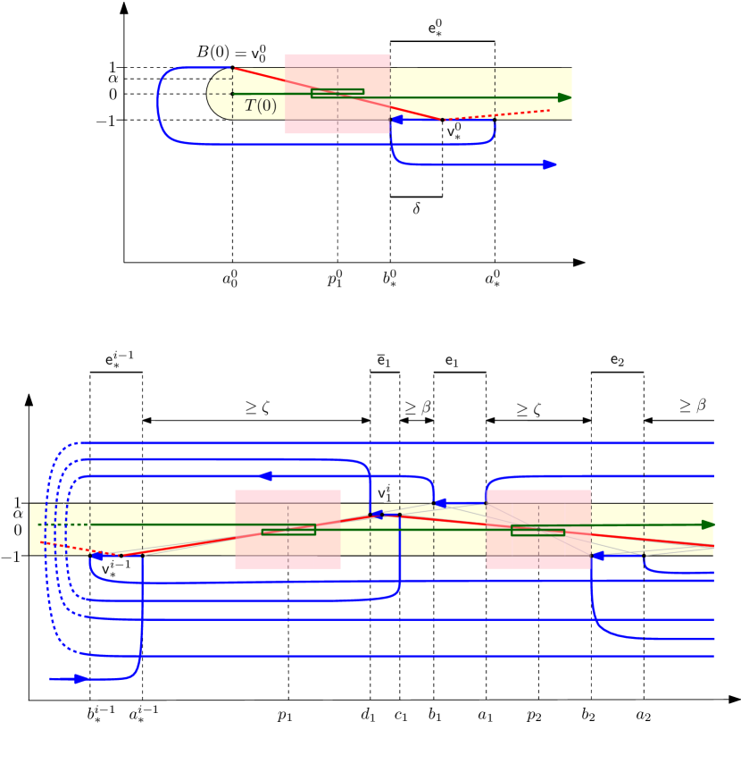
Figure 2: Top: initialization gadget $g_{0}$; bottom: the left part of split gadget $g_{i}$. The target curve is shown in green, the base curve in blue. An example shortcut curve is shown in red. Buffer zones and the hippodrome are shown as shaded regions. For the sake of presentation, the target curve is distorted to show its topology, and the lengths of the mirror edges have been assumed smaller. The top index $i$ has been omitted from the variables.

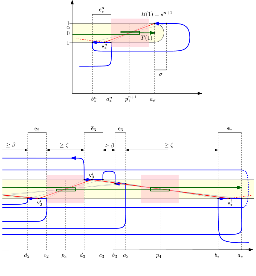
Figure 2: Top: terminal gadget $g_{n+1}$; bottom: the right part of gadget $g_{i}$ with example shortcut curve.

Initialization gadget $(g_{0})$

We let both curves start on the vertical line at $a^{0}_{0}=0$ by placing the first vertex of $T{}_{0}$ at $(a_{0}^{0},0)$ and the first vertex of the $B{}_{0}$ at $(a_{0}^{0},1)$. The base curve $B_{0}$ then continues to the left on $H_{1}$ while the target curve $T_{0}$ continues to the right on $H_{0}$. See Figure 2 (top left) for an illustration. The curve $T{}_{0}$ has one twist centered at $p_{1}^{0}=a_{0}^{0}+\gamma+\zeta/2$. The curve $B{}_{0}$ has one mirror edge $\mathsf{e}_{*}^{0}=\mathsf{a}_{*}^{0}\mathsf{b}_{*}^{0}$, which we define by setting $b_{*}^{0}=p_{1}^{0}+\zeta/2$ and $a_{*}^{0}=p_{1}^{0}+2\gamma+\zeta/2$.

Split gadgets $(g_{1},\dots,g_{n})$

The overall structure is depicted in Figure 2. The curve $B_{i}$ for $1\leq i\leq n$ has seven mirror edges. These are $\mathsf{e}_{j}^{i}=\mathsf{a}_{j}^{i}\mathsf{b}_{j}^{i}$, and $\overline{\mathsf{e}}_{j}^{i}=\mathsf{c}_{j}^{i}\mathsf{d}_{j}^{i}$, for $1\leq j\leq 3$, and the edge $\mathsf{e}_{*}^{i}=\mathsf{a}_{*}^{i}\mathsf{b}_{*}^{i}$. We connect the mirror edges using additional edges to define the following order along the base curve: $\mathsf{e}_{*}^{i-1},\mathsf{e}_{1}^{i},\overline{\mathsf{e}}_{1}^{i},\overline{\mathsf{e}}_{2}^{i},\mathsf{e}_{2}^{i},\mathsf{e}_{3}^{i},\overline{\mathsf{e}}_{3}^{i},\mathsf{e}_{*}^{i}$. The mirror edges lie on the horizontal lines $H_{1}$, $H_{-1}$ and $H_{\alpha}$. We use vertical connector edges which run in positive $y$-direction and additional connector edges which lie completely outside the hippodrome to connect the mirror edges on $H_{\alpha}$. The curve $T_{i}$ for $1\leq i\leq n$ consists of four twists centered at the projection centers $\mathsf{p}_{j}^{i}$ for $1\leq j\leq 4$ which are connected in the order of $j$ by rightward edges on $H_{0}$. To choose the exact coordinates of these points, we go through several rounds of fixing the position of the next projection center and then projecting the endpoints of mirror edges to obtain the endpoints of the next set of mirror edges. The construction is defined in four steps in Table 1 and illustrated in Figure 2 (bottom). The intuition behind this choice of projection centers is the following. In every step we make sure that the base curve stays out of the buffer zones. Furthermore, in Step 1 we choose the projection center far enough to the right such that two mirror edges located between two consecutive buffer zones have horizontal distance at least $\beta$ to each other. In Step 4 we align the projections of the two edges $\mathsf{e}_{3}^{i}$ and $\overline{\mathsf{e}}_{3}^{i}$. In this alignment, the visiting position that represents “$0$” on $\mathsf{e}_{3}^{i}$ (i.e., in its distance to $\mathsf{a}_{3}^{i}$) and the visiting position that represents “$s_{i}$” on $\overline{\mathsf{e}}_{3}^{i}$ (i.e., in its distance to $\mathsf{c}_{3}^{i}$) both project to the same point on $\mathsf{e}_{*}^{i}$ (i.e., the visiting position that represents “$s_{i}$” in its distance to $\mathsf{b}_{*}^{i}$). In this way, the projections from $\mathsf{e}_{3}^{i}$ are horizontally shifted by $s_{i}$ (scaled by $\gamma$) with respect to the projections from $\overline{\mathsf{e}}_{3}^{i}$.

Terminal gadget $(g_{n+1})$

The curve $T{}_{n+1}$ has one twist centered at $p_{1}^{n+1}=a_{*}^{n}+\zeta/2$. Let $p_{\sigma}=(b_{*}^{n}+\gamma(\sigma+1))$ and project the point $(p_{\sigma},-1)$ through $\mathsf{p}_{1}^{n+1}$ onto $H_{1}$ to obtain a point $(a_{\sigma},1)$. We finish the construction by letting both the target curve $T_{n+1}$ and the base curve $B_{n+1}$ end on a vertical line at $a_{\sigma}$. The curve $T_{n+1}$ ends on $H_{0}$ approaching from the left, while the curve $B_{n+1}$ ends on $H_{1}$ approaching from the right. Figure 2 (top right) shows an illustration.

Encoding of a subset

Any shortcut curve of the base curve encodes a subset of the SUBSET-SUM instance. We say the value $s_{i}$ is included in the encoded subset if and only if the shortcut curve visits the edge $\mathsf{e}_{1}^{i}$. The $i$th partial sum of the encoded subset will be represented by the point where the shortcut curve visits the edge $\mathsf{e}_{i}^{*}$. In particular, the distance of the visiting point to the endpoint of the edge represents this value, scaled by $\gamma$ and up to a small additive error.

3 Correctness of the reduction

Now we prove that the construction has the desired behavior. That is, we prove that any feasible shortcut curve encodes a subset that constitutes a solution to the SUBSET-SUM instance (Lemma 3.22) and for any solution of the SUBSET-SUM instance, we can construct a feasible shortcut curve (Lemma 3.16).

We call a shortcut curve one-touch if it visits any edge of the base curve in at most one point. Intuitively, for any feasible shortcut curve of $B$, there exists a one-touch shortcut curve that “approximates” it. We first prove the correctness of the reduction for this restricted type of shortcut curve (Lemma 3.16), before we turn to general shortcut curves. In Definition 1 we define a one-touch encoding, which is a one-touch shortcut curve that is feasible if and only if the encoded subset constitutes a valid solution. For such curves, Lemma 3.3 describes the correspondence of the current partial sum with the visiting position on the last edge of each gadget. It readily follows that we can construct a feasible shortcut curve from a valid solution (Lemma 3.16). For the other direction of the correctness proof we need some lemmas to testify that any feasible shortcut curve is approximately monotone (Lemma 3.8), has its vertices outside the buffer zones (Lemma 3.6), and therefore has to go through all projection centers (Lemma 3.10). We generalize Lemma 3.3 to bound the approximation error in the representation of the current partial sum (Lemma 3.20). As a result, Lemma 3.22 implies that any feasible shortcut curve encodes a valid solution.

Distance projection

In the correctness proof we often reason by using projections of distances between $H_{1}$,$H_{-1}$ and $H_{\alpha}$. The common argument is captured in the following observation.

[Distance Projection] If $\Delta_{1}$ is a triangle defined by two points $\mathsf{a}_{1}$ and $\mathsf{b}_{1}$ that lie on $H_{-1}$ and a point $\mathsf{p}$ that lies on $H_{0}$, and if $\Delta_{2}$ is a triangle defined by the points $\mathsf{p}$, and the two points $\mathsf{b}_{2}=\overline{~{}\mathsf{a}_{1}\mathsf{p}~{}}\cap H_{\alpha}$ and $\mathsf{a}_{2}=\overline{~{}\mathsf{b}_{1}\mathsf{p}~{}}\cap H_{\alpha}$, which are the projections onto $H_{\alpha}$, then it holds that $\alpha(a_{1}-b_{1})=a_{2}-b_{2}$, where $a_{1},b_{1},a_{2}$ and $b_{2}$ are the respective $x$-coordinates of the points.

3.1 Correctness for one-touch shortcut curves

We first analyze our construction under the simplifying assumption that only shortcut curves are allowed that are one-touch, i.e., shortcut curves can visit the base curve in at most one point per edge. In the next section we will build upon this analysis for the general case.

Definition 1 (One-touch encoding)

Let $I$ be an index set of a subset $S^{\prime}\subseteq S$. We construct a one-touch shortcut curve $B_{I}$ of the base curve incrementally. The first two vertices on the initial gadget are defined as follows. We choose the first vertex of the base curve $B(0)$ for $\mathsf{v}_{0}^{0}$, then we project it through the first projection center $\mathsf{p}_{1}^{0}$ onto $\mathsf{e}_{*}^{0}$ to obtain $\mathsf{v}_{*}^{0}$. Now for $i>0$, if $i\in I$, then we project $\mathsf{v}_{*}^{i-1}$ through $\mathsf{p}_{1}^{i}$ onto $\mathsf{e}_{1}^{i}$, otherwise onto $\overline{\mathsf{e}}_{1}^{i}$ to obtain $\mathsf{v}_{1}^{i}$. We continue by projecting $\mathsf{v}_{j}^{i}$ through $\mathsf{p}_{j+1}^{i}$ onto $B_{i}$ to obtain $\mathsf{v}_{j+1}^{i}$, for $1\leq j\leq 4$. Let $\mathsf{v}_{*}^{i}=\mathsf{v}_{4}^{i}$. We continue this construction throughout all gadgets in the order of $i$. Finally, we choose $B(1)=(a_{\sigma},1)$ as the last vertex of our shortcut curve. Figure 2 shows an example.

Lemma 3.1

For any $1\leq i\leq n$, it holds that $b_{4}^{i}=b_{*}^{i}+\gamma s_{i}$ and that $d_{4}^{i}=b_{*}^{i}$.

Proof 3.2

By construction, the projection center $\mathsf{p}_{4}^{i}$ lies on a common line with $\mathsf{a}_{3}^{i}$ and $\mathsf{b}_{4}^{i}$. Recall that we chose $\mathsf{p}_{4}^{i}$ such that this line intersects $H_{1}$ at the $x$-coordinate $c_{3}^{i}-\gamma s_{i}$ (see Table 1 and Figure 3). Thus, by Observation 3, it holds that $b_{4}^{i}-d_{4}^{i}=\gamma s_{i}$. Furthermore, $\mathsf{d}_{4}^{i}$ is the point with minimum $x$-coordinate out of the projections of $\mathsf{a}_{3}^{i}$, $\mathsf{b}_{3}^{i}$, $\mathsf{c}_{3}^{i}$, and $\mathsf{d}_{3}^{i}$ through $\mathsf{p}_{4}^{i}$ onto $H_{-1}$, since $\gamma s_{i}\geq 0$. Since we chose $\mathsf{b}_{*}^{i}$ as such point with minimum $x$-coordinate, the claim is implied.

Lemma 3.3

Given a shortcut curve $B_{I}$ which is a one-touch encoding (Definition 1), let $\mathsf{v}_{*}^{i}$ be the vertex of $B_{I}$ on $\mathsf{e}_{*}^{i}$, for any $0\leq i\leq n$. It holds for the distance of $\mathsf{v}_{*}^{i}$ to the endpoint of this edge that $\left\|{\mathsf{v}_{*}^{i}-\mathsf{b}_{*}^{i}}\right\|=\gamma(\sigma_{i}+1)$, where $\sigma_{i}$ is the $i$th partial sum of the subset encoded by $B_{I}$.

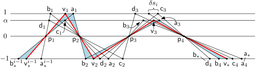
Figure 3: The path of a shortcut curve through the gadget $g_{i}$ in the case where $s_{i}$ is included in the selected set (Lemma 3.3). For presentation purposes, we allowed the mirror edges to overlap horizontally and we omitted the top index $i$ of the variables.

Proof 3.4

We prove the claim by induction on $i$. For $i=0$, the claim is true by the construction of the initialization gadget, since the partial sum $\sigma_{0}=0$ and $\left\|{\mathsf{v}_{*}^{0}-\mathsf{b}_{*}^{0}}\right\|=\gamma$. For $i>0$, there are two possibilities, either $i\in I$ or $i\notin I$. Consider the case that $s_{i}$ is included in the set encoded by $B_{I}$. In that case, the curve has to visit the edge $\mathsf{e}_{1}^{i}$.

By a repeated application of Observation 3 we can derive that

$$\left\|{\mathsf{v}_{*}^{i-1}-\mathsf{b}_{*}^{i-1}}\right\|=\left\|{\mathsf{v}_{1}^{i}-\mathsf{a}_{1}^{i}}\right\|=\left\|{\mathsf{v}_{2}^{i}-\mathsf{b}_{2}^{i}}\right\|=\frac{\left\|{\mathsf{v}_{3}^{i}-\mathsf{a}_{3}^{i}}\right\|}{\alpha}=\left\|{\mathsf{v}_{*}^{i}-\mathsf{b}_{4}^{i}}\right\|.$$

Refer to Figure 3 for an illustration of the geometry of the path through the gadget. The shaded region shows the triangles that transport the distances. Therefore, by induction and by Lemma 3.1,

$$\left\|{\mathsf{v}_{*}^{i}-\mathsf{b}_{*}^{i}}\right\|=\left\|{\mathsf{v}_{*}^{i}-\mathsf{b}_{4}^{i}}\right\|+\left\|{\mathsf{b}_{4}^{i}-\mathsf{d}_{4}^{i}}\right\|=\gamma(\sigma_{i-1}+1)+\gamma s_{i}=\gamma(\sigma_{i}+1).$$

Thus, the claim follows for the case that $s_{i}$ is selected. For the second case, the curve has to visit the edge $\overline{\mathsf{e}}_{1}^{i}$. Again, by Observation 3 it holds that

$$\left\|{\mathsf{v}_{*}^{i-1}-\mathsf{b}_{*}^{i-1}}\right\|=\frac{\left\|{\mathsf{v}_{1}^{i}-\mathsf{c}_{1}^{i}}\right\|}{\alpha}=\left\|{\mathsf{v}_{2}^{i}-\mathsf{d}_{2}^{i}}\right\|=\left\|{\mathsf{v}_{3}^{i}-\mathsf{c}_{3}^{i}}\right\|=\left\|{\mathsf{v}_{*}^{i}-\mathsf{d}_{4}^{i}}\right\|.$$

Thus $\left\|{\mathsf{v}_{*}^{i}-\mathsf{d}_{4}^{i}}\right\|=\gamma(\sigma_{i-1}+1)=\gamma(\sigma_{i}+1)$. By Lemma 3.1, $\mathsf{d}_{4}^{i}=\mathsf{b}_{*}^{i}$, thus the claim is implied also in this case.

Using the arguments from the proof of Lemma 3.3 one can derive the following corollary.

Corollary 3.5

For any $0\leq i\leq n$ the length of the edge $\mathsf{e}_{*}^{i}$ is equal to $\gamma\!\left({\sum_{1\leq j\leq i}s_{j}+2}\right)$.

Lemma 3.6

If $\alpha\in[1/2,1)$ and $\beta\geq\zeta/2$, then the base curve does not enter any of the buffer zones.

Proof 3.7

For the buffer zones centered at $\mathsf{p}_{2}^{i}$ and $\mathsf{p}_{3}^{i}$ for $1\leq i\leq n$ the claim is implied by construction. The same holds for the projection centers of the initialization gadget and the terminal gadget. Thus, we only need to argue about the first and the last projection center of the intermediate gadgets $g_{i}$ for $1\leq i\leq n$. Consider $\mathsf{p}_{1}^{i}$, by construction and since $\alpha\geq 1/2$, it holds that

$$d_{1}^{i}-p_{1}^{i}=p_{1}^{i}-\phi_{i}\geq\phi_{i}-a_{*}^{i-1}=\beta+\lambda_{i}>\beta\geq\zeta/2,$$

where $\lambda_{i}$ and $\phi_{i}$ are defined as in the construction of the gadgets. Since $d_{1}^{i}$ is the closest $x$-coordinate of the base curve to $\mathsf{p}_{1}^{i}$, the claim follows for the first projection center of a gadget.

For the last projection center, $\mathsf{p}_{4}^{i}$, we use the fact that it lies to the right of the point where the line through $\mathsf{a}_{3}^{i}$ and $\mathsf{c}_{3}^{i}$ passes through $H_{0}$. Let the $x$-coordinate of this point be denoted $c_{i}$. Now, let $\Delta_{1}$ be the triangle defined by $\mathsf{p}_{2}^{i}$, $\mathsf{d}_{1}^{i}$ and $\mathsf{c}_{1}^{i}$ and let $\Delta_{2}$ be the triangle defined by $\mathsf{p}_{3}^{i}$, $\mathsf{a}_{3}^{i}$ and $\mathsf{b}_{3}^{i}$. By the symmetry of the construction, the two triangles are the same up to reflection at the bisector between $\mathsf{p}_{2}^{i}$ and $\mathsf{p}_{3}^{i}$. Therefore,

$$p_{4}^{i}-a_{3}^{i}\geq c_{i}-a_{3}^{i}=d_{1}^{i}-p_{1}^{i}>\zeta/2,$$

and this implies the claim.

Lemma 3.8

Any feasible shortcut curve is rightwards $4$-monotone. That is, if $x_{1}$ and $x_{2}$ are the $x$-coordinates of two points that appear on the shortcut curve in that order, then $x_{2}+4\geq x_{1}$. Furthermore, it lies inside or on the boundary of the hippodrome.

Proof 3.9

Any point on the feasible shortcut curve has to lie within distance $1$ to some point of the target curve, thus the curve cannot leave the hippodrome. As for the montonicity, assume for the sake of contradiction, that there exist two points such that $x_{2}+4<x_{1}$. Let $\widehat{x}_{1}$ be the $x$-coordinate of the point on target curve matched to $x_{1}$ and let $\widehat{x}_{2}$ be the one for $x_{2}$. By the Fréchet matching it follows that $\widehat{x}_{2}-1+4<\widehat{x}_{1}+1$. This would imply that the target curve is not 2-monotone, which contradicts the way we constructed it.

Lemma 3.10

If $\alpha\in[1/2,1)$, $\zeta>4$, and $\beta\geq\zeta/2$, then a feasible shortcut curve passes through every buffer zone of the target curve via its projection center and furthermore it does so from left to right.

Proof 3.11

Any feasible shortcut curve has to start at $B(0)$ and end at $B(1)$, and all of its vertices must lie in the hippodrome or on its boundary. By Lemma 3.6 the base curve does not enter any of the buffer zones and therefore the feasible shortcut curve has to pass through the buffer zone by using a shortcut. If we choose the width of a buffer zone $\zeta>4$, then the only manner possible to do this while matching to the two associated vertices of the target curve in their respective order, is to go through the intersection of their unit disks that lies at the center of the buffer zone. This is the projection center associated with the buffer zone. By the order in which the mirror edges are connected to form the base curve, it must do so in positive $x$-direction and it must do so exactly once.

Lemma 3.12

For any $1\leq i\leq n$ it holds that $b_{1}^{i}-c_{1}^{i}\geq\beta$, $d_{2}^{i}-a_{2}^{i}\geq\beta$, and $b_{3}^{i}-c_{3}^{i}\geq\beta$.

Proof 3.13

Recall that we chose $\mathsf{p}_{1}^{i}$ by constructing the point $(\phi_{i},-\alpha)$, where $\phi_{i}=a_{*}^{i-1}+\lambda_{i}+\beta$ and $\lambda_{i}=a_{*}^{i-1}-b_{*}^{i-1}$. The construction is such that $(\phi_{i},-\alpha)$, $\mathsf{p}_{1}^{i}$ and $\mathsf{a}_{*}^{i-1}$ lie on the same line. Consider the point $(r_{i},-\alpha)$ that lies on the line through $\mathsf{b}_{*}^{i-1}$ and $\mathsf{p}_{1}^{i}$. We have that the triangle $\Delta_{1}$ defined by $(r_{i},-1)$, $\mathsf{p}_{1}^{i}$ and $\mathsf{a}_{*}^{i-1}$ is the same up to rotation as the triangle $\Delta_{2}$ defined by $(c_{1}^{i},1)$, $\mathsf{p}_{1}^{i}$ and $\mathsf{b}_{1}^{i}$. Refer to Figure 4 for an illustration. By Observation 3,

$$b_{1}^{i}-c_{1}^{i}=r_{i}-a_{*}^{i-1}=\beta+\lambda_{i}-(\phi_{i}-r_{i})\geq\beta,$$

since $(\phi_{i}-r_{i})=\alpha\lambda_{i}$. This proves the first part of the claim. Now it readily follows that also $d_{2}^{i}-a_{2}^{i}\geq\beta$. Indeed, it follows by Observation 3 that $q_{i}-a_{2}^{i}=b_{1}^{i}-c_{1}^{i}$, where $q_{i}$ is the $x$-coordinate of the projection of $(c_{1}^{i},1)$ through $\mathsf{p}_{2}^{i}$ onto $H_{-1}$, and this projection lies between $\mathsf{d}_{2}^{i}$ and $\mathsf{a}_{2}^{i}$. Again, refer to Figure 4 and in particular to triangles $\Delta_{1}^{\prime}$ and $\Delta_{2}^{\prime}$.

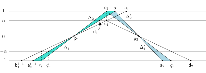
Figure 4: The geometry used in the proof of Lemma 3.12. We omitted the top index $i$ of the variables.

The claim $b_{3}^{i}-c_{3}^{i}\geq\beta$ follows from the symmetry of the middle part of the gadget. Consider the triangle $\Delta_{3}$ defined by $(c_{1}^{i},1)$, $\mathsf{p}_{2}^{i}$ and $(b_{1}^{i},1)$ and the triangle $\Delta_{4}$ defined by $(c_{3}^{i},1)$, $\mathsf{p}_{3}^{i}$ and $(b_{3}^{i},1)$. By construction $\Delta_{3}$ is a reflected version of $\Delta_{4}$, where the axis of reflection is the bisector of the two projection centers. Thus, by the above argument we have that $b_{3}^{i}-c_{3}^{i}=b_{1}^{i}-c_{1}^{i}\geq\beta$.

Lemma 3.14

If $\alpha\in[1/2,1)$, $\zeta>4$ and if $\beta>4$, then a feasible shortcut curve that is one-touch visits either $\mathsf{e}_{j}^{i}$ or $\overline{\mathsf{e}}_{j}^{i}$ for any $1\leq i\leq n$ and $1\leq j\leq 3$. Furthermore, it visits all edges $\mathsf{e}_{*}^{i}$ for $0\leq i\leq n$.

Proof 3.15

By Lemma 3.8, any feasible shortcut curve is $4$-monotone. Furthermore, it starts at $B(0)$ and ends at $B(1)$ and by Lemma 3.10, it goes through all projection centers of the target curve from left to right. We first want to argue that it visits at least one mirror edge between two projection centers, i.e., that it cannot “skip” such a mirror edge by matching to two twists in one shortcut. Such a shortcut would have to lie on $H_{0}$, since it has to go through the two corresponding projection centers lying on $H_{0}$. By construction, the only possible endpoints of such a shortcut lie on the connector edges that connect to mirror edges on $H_{\alpha}$. Assume such a shortcut could be taken by a shortcut curve starting from $B(0)$. Then, there must be a connector edge which intersects a line from a point on a mirror edge through a projection center. In particular, since the curve has to go through all projection centers, one or more of the following must be true for some $1\leq i\leq n$: (i) there exists a line through $\mathsf{p}_{1}^{i}$ intersecting a mirror edge $\mathsf{e}_{*}^{i-1}$ and a connector edge of $\overline{\mathsf{e}}_{1}^{i}$, or (ii) there exists a line through $\mathsf{p}_{3}^{i}$ intersecting a mirror edge $\mathsf{e}_{2}^{i}$ or $\overline{\mathsf{e}}_{2}^{i}$ and a connector edge of $\mathsf{e}_{3}^{i}$. However, this was prevented by the careful placement of these connector edges.

It remains to prove that the shortcut curve cannot visit both $\mathsf{e}_{j}^{i}$ and $\overline{\mathsf{e}}_{j}^{i}$ for any $i$ and $j$, and therefore visits at most one mirror edge between two projection centers. First of all, the shortcut curve has to lie inside or on the boundary of the hippodrome and is $4$-monotone (Lemma 3.8). At the same time, we constructed the gadget such that the mirror edges between two consecutive projection centers have distance at least $\beta$ by Lemma 3.12 and that the left mirror edge comes after the right mirror edge along their order of $B$. Since we chose $\beta>4$, the shortcut curve cannot visit both mirror edges.

Putting the above lemmas together implies the correctness of the reduction for shortcut curves that are one-touch, i.e., which visit every edge in at most one point.

Lemma 3.16

If $\alpha\in[1/2,1)$, $\zeta>4$ and if $\beta>4$, then for any feasible one-touch shortcut curve $B_{\Diamond}$, it holds that the subset encoded by $B_{\Diamond}$ sums to $\sigma$. Furthermore, for any subset of $s$ that sums to $\sigma$, there exists a feasible one-touch shortcut curve that encodes it.

Proof 3.17

Lemma 3.14 and Lemma 3.10 imply that $B_{\Diamond}$ must be a one-touch encoding as defined in Definition 1 if it is feasible. By Lemma 3.3, the second last vertex of $B_{\Diamond}$ is the point on the edge $\mathsf{e}_{*}^{n}$, which is in distance $\gamma(\sigma_{\Diamond}+1)$ to $\mathsf{b}_{*}^{n}$, where $\sigma_{\Diamond}$ is the sum encoded by the subset selected by $B_{\Diamond}$. The last vertex of $B_{\Diamond}$ is equal to $B(1)$, which we placed in distance $\gamma(\sigma+1)$ to the projection of $\mathsf{b}_{*}^{n}$ through $\mathsf{p}_{1}^{n+1}$. Thus, if and ony if $\sigma_{\Diamond}=\sigma$, then the last shortcut of $B_{\Diamond}$ passes through the last projection center of the target curve. It follows that if $\sigma_{\Diamond}\neq\sigma$, then $B_{\Diamond}$ cannot be feasible. For the second part of the claim, we construct a one-touch encoding as defined in Definition 1. By the above analysis, it will be feasible if the subset sums to $\sigma$, since the curve visits every edge of $B$ in at most one point and in between uses shortcuts which pass through every buffer zone from left to right and via the buffer zone’s projection center.

3.2 Size of the construction

We prove that the construction has polynomial size.

Lemma 3.18

The curves can be constructed in $O(n)$ time. Furthermore, if we choose $\alpha=1/2,\beta=5$, $\zeta=5$, and $\gamma=25n$, then the size of the coordinates used is in $O(\log n+\log(\sum_{i=0}^{n}s_{i}))$.

Proof 3.19

Each of the constructed gadgets uses a constant number of vertices. Since we construct $n+2$ gadgets, the overall number of vertices used is in $O(n)$. The curves can be constructed using a single iteration from left to right, therefore they can be constructed in $O(n)$ time.

Secondly, we can bound the size of the coordinates as follows. We claim that

$$a_{\sigma}\in O\!\left({n^{2}\sum_{i=0}^{n}s_{i}}\right)$$ (1)

Using basic geometry, we can bound the horizontal length of an individual split gadget as follows. Let $A_{i}=p_{1}^{i}-a_{*}^{i-1}$. Let $\lambda_{i}=a_{*}^{i-1}-b_{*}^{i-1}$ as defined as in Table 1 (see also Figure 2).

$$a_{*}^{i}-a_{*}^{i-1} =(a_{*}^{i}-b_{1}^{i})+(b_{1}^{i}-p_{1}^{i})+(p_{1}^{i}-a_{*}^{i-1})$$

$$=(a_{*}^{i}-b_{1}^{i})+2A_{i}$$

$$=(a_{*}^{i}-p_{2}^{i})+(p_{2}^{i}-b_{1}^{i})+2A_{i}$$

$$=(a_{*}^{i}-p_{2}^{i})+\lambda_{i}+\zeta/2+2A_{i}$$

$$=(a_{*}^{i}-c_{2}^{i})+(c_{2}^{i}-p_{2}^{i})+\lambda_{i}+\zeta/2+2A_{i}$$

$$\leq(a_{*}^{i}-c_{2}^{i})+\!\left({\frac{p_{2}^{i}-d_{1}^{i}}{\alpha}}\right)+\lambda_{i}+\zeta/2+2A_{i}$$

$$=(a_{*}^{i}-c_{2}^{i})+\!\left({\frac{A_{i}+\lambda_{i}+\zeta/2}{\alpha}}\right)+\lambda_{i}+\zeta/2+2A_{i}$$

$$\leq(a_{*}^{i}-c_{2}^{i})+4A_{i}+3\lambda_{i}+2\zeta$$

$$=(a_{*}^{i}-d_{3}^{i})+(d_{3}^{i}-c_{2}^{i})+4A_{i}+3\lambda_{i}+2\zeta$$

$$=(a_{*}^{i}-d_{3}^{i})+4A_{i}+3\lambda_{i}+3\zeta$$

$$=(a_{*}^{i}-p_{4}^{i})+(p_{4}^{i}-d_{3}^{i})+4A_{i}+3\lambda_{i}+3\zeta$$

$$\leq 2\!\left({\frac{a_{3}^{i}-d_{3}^{i}+\gamma s_{i}}{1-\alpha}}\right)+4A_{i}+3\lambda_{i}+3\zeta$$

$$\leq 2\!\left({\frac{A_{i}+\lambda_{i}+\gamma s_{i}}{1-\alpha}}\right)+4A_{i}+3\lambda_{i}+3\zeta$$

$$=8A_{i}+7\lambda_{i}+4\gamma s_{i}+3\zeta$$

By the construction of the first projection center in Table 1, it holds that

$$A_{i}\leq\frac{\beta+\lambda_{i}}{1-\alpha}=2(\beta+\lambda_{i})$$

Putting everything together, we get

$$a_{\sigma} =(a_{\sigma}-a_{*}^{n})+\sum_{i=1}^{n}(a_{*}^{i}-a_{*}^{i-1})+a_{*}^{0}$$

$$\leq(2\lambda_{n+1}+\zeta)+\sum_{i=1}^{n}(a_{*}^{i}-a_{*}^{i-1})+(\zeta+3\gamma)$$

$$\leq 2\lambda_{n+1}+\zeta+\sum_{i=1}^{n}\!\left({16\!\left({\beta+\lambda_{i}}\right)+7\lambda_{i}+4\gamma s_{i}+3\zeta}\right)+\zeta+3\gamma$$

$$\leq 23\sum_{i=1}^{n+1}\lambda_{i}+4\gamma\sum_{i=1}^{n}s_{i}+16n\beta+3(n+1)\zeta+3\gamma$$

By construction of the initialization gadget, it holds that $\lambda_{1}=2\gamma$. Together with this implies that

$$\lambda_{i}\leq\gamma\!\left({\sum_{i=1}^{n}s_{j}+2}\right)$$

for $1\leq i\leq n+1$. Since we chose $\gamma=25n$ and the remaining global variables constant, the claim is implied.

3.3 Correctness for general shortcut curves

Next, we generalize Lemma 3.3 to bound the incremental approximation error of the visiting positions on the last edge of each gadget for general shortcut curves, that is, assuming shortcut curves are not necessarily one-touch.

Lemma 3.20

Choose $\alpha\in[1/2,1)$, $\zeta>4$ and $\beta>4$. Given a feasible shortcut curve $B_{\Diamond}$, let $\mathsf{v}_{*}^{i}$ be any point of $B_{\Diamond}$ on $\mathsf{e}_{*}^{i}$ and let $v_{*}^{i}$ denote its $x$-coordinate. For any $0\leq i\leq n$ let $\sigma_{i}$ denote the $i$th partial sum of the subset encoded by $B_{\Diamond}$. If we choose $\gamma>{\varepsilon}_{i}$, then it holds that

$$b_{*}^{i}+\gamma_{i}-{\varepsilon}_{i}\leq v_{*}^{i}\leq b_{*}^{i}+\gamma_{i}+{\varepsilon}_{i}$$

where $\gamma_{i}=\gamma(\sigma_{i}+1)$ and ${\varepsilon}_{i}=\frac{8i+4}{\alpha}$.

Proof 3.21

We prove the claim by induction on $i$. For $i=0$ the claim follows by the construction of the initialization gadget. Indeed, the curve $B_{\Diamond}$ has to start at $B(0)=\mathsf{a}_{0}^{0}$ and by Lemma 3.10 it has to pass through both $\mathsf{p}_{1}^{0}$ and $\mathsf{p}_{1}^{1}$. Since the three points $\mathsf{a}_{0}^{0},\mathsf{p}_{1}^{0},$ and $\mathsf{p}_{1}^{1}$ do not lie on a common line, there must be an edge of the base curve in between the two projection centers visited by $B_{\Diamond}$. By Lemma 3.8, the shortcut curve cannot leave the hippodrome. However, the only edge available in the hippodrome is $\mathsf{e}_{*}^{0}$. By construction, the only possible shortcut to this edge ends at the center of the edge in distance $\gamma$ to ${\mathsf{b}_{*}^{0}}$. Since the mirror edge runs leftwards, the only other points that can be visited by $B_{\Diamond}$ lie therefore in this direction. However, by Lemma 3.8, $B_{\Diamond}$ is rightwards $4$-monotone. It follows that

$$b_{*}^{0}+\gamma-4\leq v_{*}^{0}\leq b_{*}^{i}+\gamma.$$

Since ${\varepsilon}_{0}=4/\alpha>4$ and $\sigma_{0}=0$, this implies the claim for $i=0$.

For $i>0$, the curve $B_{\Diamond}$ entering gadget $g_{i}$ from the edge $\mathsf{e}_{*}^{i-1}$ has to pass through the first buffer zone via the projection center $p_{1}^{i}$. By induction,

$$b_{*}^{i-1}+\gamma_{\min}~{}\leq~{}v_{*}^{i-1}~{}\leq~{}b_{*}^{i-1}+\gamma_{\max},$$

where $\gamma_{\min}=\gamma_{i-1}-{\varepsilon}_{i-1}$ and $\gamma_{\max}=\gamma_{i-1}+{\varepsilon}_{i-1}$ denote the minimal and maximal distances of the visiting position to the left endpoint on the edge $\mathsf{e}_{*}^{i-1}$. Since $\gamma>{\varepsilon}_{i}={\varepsilon}_{i-1}+8/\alpha$, and $\sigma_{i-1}\geq 0$, it follows that

$$\gamma_{\min}=\gamma(\sigma_{i-1}+1)-{\varepsilon}_{i-1}\geq\gamma-{\varepsilon}_{i-1}>8/\alpha.$$ (2)

Furthermore, by ,

$$\gamma_{\max}\leq\gamma\!\left({\sum_{1\leq j\leq i-1}s_{j}+1}\right)+{\varepsilon}_{i-1}\leq\!\left({\lambda_{i}-\gamma}\right)+{\varepsilon}_{i-1}\leq\lambda_{i}-8/\alpha,$$ (3)

where $\lambda_{i}=a_{*}^{i-1}-b_{*}^{i-1}$ is the length of edge $\mathsf{e}_{*}^{i-1}$. Thus, $\mathsf{v}_{*}^{i-1}$ lies at distance at least $8/\alpha$ from each endpoint of $\mathsf{e}_{*}^{i-1}$. Therefore, the only two edges of the base curve which intersect the line $\overline{~{}\mathsf{v}_{*}^{i-1}\mathsf{p}_{1}^{i}~{}}$ within the hippodrome are $\mathsf{e}_{1}^{i}$ and $\overline{\mathsf{e}}_{1}^{i}$. Note that also the vertical connector edges at $\overline{\mathsf{e}}_{1}^{i}$ do not intersect any such line within the hippodrome.

Now, there are two cases, either the shortcut ends on $\mathsf{e}_{1}^{i}$ or on $\overline{\mathsf{e}}_{1}^{i}$. Assume the latter case. By Observation 3 the $x$-coordinate of the endpoint of the shortcut lies in the interval

$$\!\!\left[{c_{1}^{i}-\alpha\gamma_{\max}~{},~{}c_{1}^{i}-\alpha\gamma_{\min}}\rule[-5.69046pt]{0.0pt}{11.38092pt}\right].$$

By the same observation, the length of the edge $\overline{\mathsf{e}}_{1}^{i}$ is equal to $\alpha\lambda_{i}$. Thus, the endpoint of the shortcut lies inside the edge.

We now argue that the shortcut curve has to leave the edge by using a shortcut, i.e., the shortcut curve cannot “walk” out of the edge by using a subcurve of $B$. The mirror edges are oriented leftwards. Since the shortcut curve has to be rightwards $4$-monotone (Lemma 3.8), it can only walk by a distance $4$ on each such edge. Let $\mathcal{I}_{j}^{i}$ denote the range of $x$-coordinates of $B_{\Diamond}$ on $\overline{\mathsf{e}}_{j}^{i}$. By the above,

$$\mathcal{I}_{1}^{i}\subseteq\!\!\left[{c_{1}^{i}-\alpha\gamma_{\max}-4~{},~{}c_{1}^{i}-\alpha\gamma_{\min}}\rule[-5.69046pt]{0.0pt}{11.38092pt}\right]$$

Thus, by Eq. (3) and Eq. (2) and since $c_{1}^{i}-d_{1}^{i}=\alpha\lambda_{i}$, it holds that $\mathcal{I}_{1}^{i}\subseteq[d_{1}^{i},c_{1}^{i}]$, i.e., the shortcut curve must leave the edge $\overline{\mathsf{e}}_{1}^{i}$ by using a shortcut. A shortcut to $\mathsf{e}_{1}^{i}$ would violate the order along the base curve $B$. Since the shortcut curve is rightwards $4$-monotone (Lemma 3.8) and must pass a through a buffer zone via its projection center (Lemma 3.10), the only way to leave the edge is to take a shortcut through $\mathsf{p}_{2}^{i}$. The only edge intersecting a line through $\mathsf{p}_{2}^{i}$ and a point on $\overline{\mathsf{e}}_{1}^{i}$ is $\overline{\mathsf{e}}_{2}^{i}$. Thus, $\overline{\mathsf{e}}_{2}^{i}$ must be the next edge visited. Now we can again use Observation 3 to project the set of visiting points onto the next edge and use the fact that the shortcut curve can only walk rightwards and only by a distance at most $4$ on a mirror edge to derive that

$$\mathcal{I}_{2}^{i}\subseteq\!\!\left[{d_{2}^{i}+\gamma_{\min}-4~{},~{}d_{2}^{i}+(\gamma_{\max}+4/\alpha)}\rule[-5.69046pt]{0.0pt}{11.38092pt}\right]\subseteq[d_{2}^{i},c_{2}^{i}].$$

By repeated application of the above arguments, we obtain that $\overline{\mathsf{e}}_{3}^{i}$ is visited within

$$\mathcal{I}_{3}^{i}\subseteq\!\!\left[{c_{3}^{i}-(\gamma_{\max}+4/\alpha)-4~{},~{}c_{3}^{i}-(\gamma_{\min}-4)}\rule[-5.69046pt]{0.0pt}{11.38092pt}\right]\subseteq[d_{3}^{i},c_{3}^{i}],$$

and that $\overline{\mathsf{e}}_{*}^{i}$ is visited within

$$\mathcal{I}_{*}^{i}\subseteq\!\!\left[{d_{4}^{i}+(\gamma_{\min}-4)-4~{},~{}d_{4}^{i}+(\gamma_{\max}+4/\alpha+4)}\rule[-5.69046pt]{0.0pt}{11.38092pt}\right]\subseteq[d_{4}^{i},c_{4}^{i}]\subseteq[b_{*}^{i},a_{*}^{i}]$$

For each visited edge, it follows by Eq. (3) and Eq. (2) that the shortcut curve visits the edge in the interior.

Now, since the shortcut curve did not visit $\mathsf{e}_{1}^{i}$, the input value $s_{i}$ is not included in the selected subset, therefore $\gamma_{i}=\gamma_{i-1}$. Using the interval $\mathcal{I}_{*}^{i}$ derived above, and the fact that $d_{4}^{i}=b_{*}^{i}$ (Lemma 3.1) it follows that

$$v_{*}^{i}~{}\geq~{}d_{4}^{i}+\gamma_{\min}-8~{}\geq~{}d_{4}^{i}+(\gamma_{i-1}-{\varepsilon}_{i-1})-8\geq b_{*}^{i}+\gamma_{i}-{\varepsilon}_{i},$$

and similarly,

$$v_{*}^{i}\leq d_{4}^{i}+\gamma_{\max}+8/\alpha\leq d_{4}^{i}+(\gamma_{i-1}+{\varepsilon}_{i-1})+8/\alpha\leq b_{*}^{i}+\gamma_{i}+{\varepsilon}_{i}$$

Thus, the claim follows in the case that $B_{\Diamond}$ visits $\overline{\mathsf{e}}_{1}^{i}$.

The case that $B_{\Diamond}$ visits $\mathsf{e}_{1}^{i}$ can be proven along the same lines. However, now $s_{i}$ is included in the selected subset, and therefore $\gamma_{i}=\gamma_{i-1}+\gamma s_{i}$. Using the arguments above we can derive

$$\mathcal{I}_{*}^{i}\subseteq\!\!\left[{b_{4}^{i}+\gamma_{\min}-8/\alpha~{},~{}b_{4}^{i}+\gamma_{\max}+8/\alpha}\rule[-5.69046pt]{0.0pt}{11.38092pt}\right]$$

By Lemma 3.1, $b_{4}^{i}=b_{*}^{i}+\gamma s_{i}$. (Note that the same argument was used in Lemma 3.3). Thus, analogous to the above

$$v_{*}^{i}\geq b_{4}^{i}+\gamma_{i-1}-{\varepsilon}_{i}\geq b_{*}^{i}+\gamma s_{i}+\gamma_{i-1}-{\varepsilon}_{i}\geq b_{*}^{i}+\gamma_{i}-{\varepsilon}_{i}$$

and similarly,

$$v_{*}^{i}\leq b_{4}^{i}+\gamma_{i-1}+{\varepsilon}_{i}\leq b_{*}^{i}+\gamma s_{i}+\gamma_{i-1}+{\varepsilon}_{i}\leq b_{*}^{i}+\gamma_{i}+{\varepsilon}_{i}$$

Therefore the claim is implied also in this case.

Lemma 3.22

If we choose $\alpha\in[1/2,1),\beta>4$, $\zeta>4$, and $\gamma\geq 25n$, then any feasible shortcut curve $B_{\Diamond}$ encodes a subset of $\left\{{s_{1},\dots,s_{n}}\right\}$ that sums to $\sigma$.

Proof 3.23

Since $B_{\Diamond}$ is feasible, it must be that it visits $\mathsf{e}_{*}^{n}$ at distance $\gamma(\sigma+1)$ to $\mathsf{b}_{*}^{n}$, since this is the only point to connect via a shortcut through the last projection center to the endpoint of $B$ and by Lemma 3.10 all projection centers have to be visited. So let $v_{*}^{n}=b_{*}^{n}+\gamma(\sigma+1)$ be the $x$-coordinate of this visiting point (the starting point of the last shortcut), and let $\sigma_{n}$ be the sum of the subset encoded by $B_{\Diamond}$. Lemma 3.20 implies that

$$b_{*}^{n}+\gamma(\sigma_{n}+1)-{\varepsilon}_{n}\leq b_{*}^{n}+\gamma(\sigma+1)\leq b_{*}^{n}+\gamma(\sigma_{n}+1)+{\varepsilon}_{n},$$

since ${\varepsilon}_{n}=\frac{8n+4}{\alpha}<25n=\gamma$. Therefore,

$$\sigma_{n}-{\varepsilon}_{n}/\gamma\leq\sigma\leq\sigma_{n}+{\varepsilon}_{n}/\gamma$$

For our choice of parameters ${\varepsilon}_{n}/\gamma<1$. Thus, it must be that $\sigma=\sigma_{n}$, since both values are integers.

3.4 Main result

Now, together with Lemma 3.16 and the fact that the reduction is polynomial (Lemma 3.18), Lemma 3.22 implies the NP-hardness of the problem.

Theorem 3.24

The problem of deciding whether the shortcut Fréchet distance between two given curves is less or equal a given distance is NP-hard.

4 Algorithms

We give two $O(n^{3}\log n)$ time algorithms for deciding the shortcut Fréchet distance. One is a $3$-approximation algorithm for the general case, and one an exact algorithm for the vertex-restricted case. Both algorithms traverse the free space as usual, using a line stabbing algorithm by Guibas et al. [14] to test the admissability of shortcuts.

The approximation algorithm for the general case uses a crucial lemma of Driemel and Har-Peled [12] to approximate the reachable free space and prevent it from fragmenting. The exact algorithm for the vertex-restricted case uses a similar lemma for efficiently testing all possible shortcuts. In this case, the free space naturally does not fragment.

First we discuss relevant preliminaries, in particular tunnels in the free space diagram and ordered line-stabbing.

4.1 Preliminaries

Free space Diagram

Let $T,B$ be two polygonal curves parameterized over $[0,1]$. The standard way to compute the Fréchet distance uses the $\delta$-free space of $T$ and $B$, which is a subset of the joint parametric space of $T$ and $B$, defined as

$$\mathcal{D}_{\leq\delta}(T,B)=\left\{{(x,y)\in[0,1]^{2}\,\left|\,{\left\|{T(x)-B(y)}\right\|\leq\delta}\rule[-5.69046pt]{0.0pt}{11.38092pt}\right.}\right\}.$$

From now on, we will simply write $\mathcal{D}_{\leq\delta}$. The square $[0,1]^{2}$, which represents the joint parametric space, can be broken into a (not necessarily uniform) grid called the free space diagram, where a vertical line corresponds to a vertex of $T$ and a horizontal line corresponds to a vertex of $B$.

Every pair of segments of $T$ and $B$ define a cell in this grid. Let $C_{i,j}$ denote the cell that corresponds to the $i$th edge of $T$ and the $j$th edge of $B$. The cell $C_{i,j}$ is located in the $i$th column and $j$th row of this grid. It is known that the free space, for a fixed $\delta$, inside such a cell $C_{i,j}$ (i.e., $\mathcal{D}_{\leq\delta}\cap C_{i,j}$) is convex [3]. We will denote it with $\mathcal{D}_{\leq\delta}^{(i,j)}$.

Furthermore, the Fréchet distance between two given curves is less or equal to $\delta$ if and only if there exists a monotone path in the free space that starts in the lower left corner $(0,0)$ and ends in the upper right corner $(1,1)$ of the free space diagram [3]. For the shortcut Fréchet distance, we need to also allow shortcuts. This is captured in the concept of tunnels in free space. A shortcut segment $\overline{B}\!\left[\rule[0.0pt]{0.0pt}{9.95863pt}{y_{\mathsf{p}},y_{\mathsf{q}}}\right]$ and the subcurve ${T}\left[\rule[0.0pt]{0.0pt}{9.95863pt}{x_{\mathsf{p}},x_{\mathsf{q}}}\right]$ it is being matched to, correspond in the parametric space to a segment $\mathsf{p}\mathsf{q}\subseteq[0,1]^{2}$, called a tunnel and denoted by $\mathsf{\tau}\!\left({\mathsf{p},\mathsf{q}}\right)$, where $\mathsf{p}=\!\left({x_{\mathsf{p}},y_{\mathsf{p}}}\right)$ and $\mathsf{q}=\!\left({x_{\mathsf{q}},y_{\mathsf{q}}}\right)$. We require $x_{\mathsf{p}}\leq x_{\mathsf{q}}$ and $y_{\mathsf{p}}\leq y_{\mathsf{q}}$ for monotonicity. We call the Fréchet distance of the shortcut segment to the subcurve the price of this tunnel and denote it with ${\mathrm{p{r}c}}_{\mathsf{\tau}}\!\left({\mathsf{p},\mathsf{q}}\right)=\mathsf{d}_{\mathcal{F}}\!\left({{T}\left[\rule[0.0pt]{0.0pt}{9.95863pt}{x_{\mathsf{p}},x_{\mathsf{q}}}\right],\overline{B}\!\left[\rule[0.0pt]{0.0pt}{9.95863pt}{y_{\mathsf{p}},y_{\mathsf{q}}}\right]}\right)$. A tunnel $\mathsf{\tau}\!\left({\mathsf{p},\mathsf{q}}\right)$ is feasible for $\delta$ if $\mathsf{p},\mathsf{q}\in\mathcal{D}_{\leq\delta}({T},{B})$.

Now, we define the reachable free space, as follows

$$\mathcal{R}_{\leq\delta}\!\left({T,B}\right)=\left\{{(x_{\mathsf{p}},y_{\mathsf{p}})\in[0,1]^{2}\,\left|\,{\mathsf{d}_{\mathcal{S}}\!\left({{T}\left[\rule[0.0pt]{0.0pt}{9.95863pt}{0,x_{\mathsf{p}}}\right],{B}\left[\rule[0.0pt]{0.0pt}{9.95863pt}{0,y_{\mathsf{p}}}\right]}\right)\leq\delta}\rule[-5.69046pt]{0.0pt}{11.38092pt}\right.}\right\}.$$

From now on, we will simply write $\mathcal{R}_{\leq\delta}$. This is the set of points that have an $(x,y)$-monotone path from $(0,0)$ that stays inside the free space and otherwise uses tunnels. We will denote the reachable space inside a cell (i.e., $\mathcal{R}_{\leq\delta}\cap C_{i,j}$) with $\mathcal{R}_{\leq\delta}^{(i,j)}$.

Finally, we will use the following well-known fact, that the Fréchet distance between two line segments is the maximum of the distance of the endpoints. Given segments $\mathsf{a}\mathsf{b}$ and $\mathsf{c}\mathsf{d}$, it holds $\mathsf{d}_{\mathcal{F}}\!\left({\mathsf{a}\mathsf{b},\mathsf{c}\mathsf{d}}\right)=\max(\left\|{\mathsf{c}-\mathsf{a}}\right\|$, $\left\|{\mathsf{d}-\mathsf{b}}\right\|)$.

Monotonicity of tunnel prices

In order to prevent the reachable space from being fragmented, as it is the case with the exact problem we showed to be NP-hard, we will approximate it. For this, we will use the following lemma from [12].

Lemma 4.1 ([12])

Given a value $\delta>0$ and two curves ${T}_{1}$ and ${T}_{2}$, such that ${T}_{2}$ is a subcurve of ${T}_{1}$, and given two line segments $\overline{B}_{1}$ and $\overline{B}_{2}$, such that $\mathsf{d}_{\mathcal{F}}\!\left({{T}_{1},\overline{B}_{1}}\right)\leq\delta$ and the start (resp. end) point of ${T}_{2}$ is in distance $\delta$ to the start (resp. end) point of ${\overline{B}_{2}}$, then $\mathsf{d}_{\mathcal{F}}\!\left({{T}_{2},\overline{B}_{2}}\right)\leq 3\delta$.

Horizontal, vertical and diagonal tunnels

We can distinguish three types of tunnels. We call a tunnel that stays within a column of the grid, a vertical tunnel. Likewise, a tunnel that stays within a row is called a horizontal tunnel. Tunnels that span across rows and columns are diagonal tunnels. Note that vertical tunnels that are feasible for a value of $\delta$ also have a price at most $\delta$ by Observation 4.1. Furthermore, the shortcut which corresponds to a horizontal tunnel lies within an edge of the input curve. Thus, shortcutting the curve does not have any effect in this case and we can safely ignore such horizontal tunnels.

Ordered line stabbing

Guibas et al. [14] study the problem of stabbing an ordered set of unit radius disks with a line. In particular, one of the problems studied is the following. Given a series of unit radius disks $D_{1},\dots,D_{n}$, does there exist a directed line $\ell$, with $n$ points $\mathsf{p}_{i}$, which lie along $\ell$ in the order of $i$, such that $\mathsf{p}_{i}\in D_{i}$? As was already noted by Guibas et al., their techniques can be applied to decide whether there exists a line segment that lies within Fréchet distance one to a given polygonal curve $X$. Simply center the disks at the vertices of $X$ in their order along the curve and the relationship follows from the fact that the Fréchet distance between two line segments is the maximum of the distances of their endpoints.

The algorithm described by Guibas et al. maintains a so called line-stabbing wedge that contains all points $\mathsf{p}$, such that there is a line through $\mathsf{p}$ that visits the first $i$ disks before visiting $\mathsf{p}$. The algorithm runs in $O(n\log n)$ time. We will use this algorithm, to compute all tunnels of price at most $\delta$ starting from a particular point in the parametric space and ending in a particular cell.

4.2 Approximate decision algorithm

We describe an approximate decision algorithm for the directed continuous shortcut Fréchet distance. Given a value of $\delta$ and two polygonal curves $T$ and $B$ in ${\rm I\!R}^{2}$ of total complexity $n=n_{1}+n_{2}$, the algorithm outputs either (i) ”$d_{\mathcal{S}}\!\left({T,B}\right)\leq 3\delta$“, or (ii) ”$d_{\mathcal{S}}\!\left({T,B}\right)>\delta$“. The algorithm runs in $O(n^{3}\log n)$ time and $O(n)$ space. We first discuss the challenges and then give a sketch of the algorithm.

4.2.1 Challenge and ideas

The standard way to solve the decision problem for the Fréchet distance and its variants is to search for monotone paths in the free space diagram. In the case of the shortcut Fréchet distance, this path can now use tunnels in the free space diagram, which correspond to shortcuts on $B$ which are matched to subcurves of $T$. In the general version of the shortcut Fréchet distance, the tunnels can now start and end anywhere inside the free space cells, while in the vertex-restricted case they are constrained to the grid of the parametric space. In order to extend the algorithm by Driemel and Har-Peled [12] to this case, we need a new method to compute the space which is reachable within a free space cell.

We use the concept of line-stabbing to compute all tunnels $\mathsf{\tau}\!\left({\mathsf{p},\mathsf{q}}\right)$ of price at most $\delta$ starting from a particular point $\mathsf{p}$ in the parametric space and ending in a particular cell. By intersecting the line-stabbing wedge with the edge of $B$ that corresponds to the cell, we obtain a horizontal strip which represents the set of such tunnel endpoints $\mathsf{q}$. See Figure 5 for an illustration.

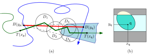
Figure 5: (a) Example of a tunnel $\mathsf{\tau}\!\left({\mathsf{p},\mathsf{q}}\right)$ computed by the diagonalTunnel procedure. The shaded area shows the line-stabbing wedge. (b) The free space cell which contains the endpoint of the tunnel.

The second challenge is that the reachable free space can fragment into exponentially many of such horizontal strips. However, we can exploit the monotonicity of the tunnel prices to approximate the reachable free space as done in the algorithm by Driemel and Har-Peled. In this approximation scheme, the combinatorial complexity of the reachable space is constant per cell. Thus, the overall complexity is bounded by $O(n^{2})$. Our algorithm takes $O(n\log n)$ time per cell, resulting in $O(n^{3}\log n)$ time overall.

Driemel and Har-Peled make certain assumptions on the input curves and achieve a near-linear running time. Instead of traversing $O(n^{2})$ cells, they considered only those cells that intersect the free space on their boundary. To compute these cells, a data structure of de Berg and Streppel [10] was used. Unfortunately, this method does not immediately extend to our case, since we also need to consider cells that intersect the free space in their interior only. Therefore, our algorithm traverses the entire free space diagram yielding a much simpler, yet slower algorithm, without making assumptions on the input curves.

4.2.2 Sketch

We traverse the free space as usual to compute the reachable free space. In each cell, in addition to the reachable free space from neighboring cells, we also compute the free space reachable by a shortest tunnel at price $3\delta$. For this, we store (or find) the right-most point in the free space below and to the right of the current cell, i.e., the point that will give the shortest tunnel. We modify the line-stabbing algorithm of Guibas et al. to compute the free space reachable by a tunnel from this point (see diagonalTunnel below). Now, by the lemma of Driemel and Har-Peled, we know that any point not reachable by a shortest tunnel at price $3\delta$ is also not reachable by a longer tunnel at price $\delta$. Because we compute reachability by only one tunnel, the free space fragments only in a constant number of pieces. In this way, we obtain a $3$-approximation to the decision version of the problem.

4.2.3 The tunnel procedures

The diagonalTunnel procedure receives as input a cell $C_{i,i}$ and a point $\mathsf{p}\in\mathcal{D}_{\leq\delta}$, such that $\mathsf{p}$ lies in the lower left quadrant of the lower left corner of the cell $C_{i,i}$ and a parameter $\delta>0$. The output will be a set of points ${\mathsf{P}}\subseteq C_{i,i}$, such that ${\mathrm{p{r}c}}_{\mathsf{\tau}}\!\left({\mathsf{p},\mathsf{q}}\right)\leq\delta$ if and only if $\mathsf{q}\in{\mathsf{P}}$. We use the line-stabbing algorithm mentioned above with minor modifications. Let $x_{\mathsf{p}}=x_{-}$ be the $x$-coordinate of $\mathsf{p}$ and let $x_{+}$ be the $x$-coordinate of some point in the interior of $C_{i,i}$. Let $D_{1},\dots,D_{k}$ be the disks of radius $\delta$ centered at the vertices of $T$ that are spanned by the subcurve ${T}\left[\rule[0.0pt]{0.0pt}{9.95863pt}{x_{-},x_{+}}\right]$. There are two cases, either $B(y_{\mathsf{p}})$ is contained in $D_{i}$ for all $1\leq i\leq k$, or there exists some $i$, such that $B(y_{\mathsf{p}})$ lies outside of $D_{i}$. In the first case, we return ${\mathsf{P}}=C_{i,i}\cap\mathcal{D}_{\leq\delta}$. In the second case we initialize the line-stabbing wedge of [14] with the tangents of $B(y_{\mathsf{p}})$ to the disk $D_{i}$, where $i$ is the smallest index such that $B(y_{\mathsf{p}})\notin D_{i}$. We then proceed with the algorithm as written by handling the disks $D_{i+1},\dots,D_{k}$. Finally, we intersect the line-stabbing wedge with the edge of B that corresponds to $C_{i,i}$. Refer to Figure 5 for an illustration. This yields a horizontal slab of points that lie in $C_{i,i}$ which we then intersect with the $\delta$-free space and return as our set ${\mathsf{P}}$.

The verticalTunnel procedure receives as input a cell $C_{i,i}$ and a point $\mathsf{p}$ which lies below this cell in the same column and a parameter $\delta\geq 0$. Let $H_{\mathsf{p}}$ be the closed halfplane which lies to the right of the vertical line through $\mathsf{p}$. The procedure returns the intersection of $H_{\mathsf{p}}$ with the $\delta$-free space in $C_{i,i}$.

Decider$(T,B,\delta)$ 1:  Assert that $\mathsf{d}\!\left({0,0}\right)=\left\|{T(0)-B(0)}\right\|\leq\delta$ and $\mathsf{d}\!\left({1,1}\right)\leq\delta$ 2:  Let ${}\mathcal{A}$, ${}\overline{\mathcal{A}}$, ${}g^{\ell}$, ${}\overline{g}^{\ell}$, ${}g^{r}$, and ${}\overline{g}^{r}$ be arrays of size $n_{1}$ 3:  for $j=1,\dots,n_{2}$ do 4:     Update ${}\overline{\mathcal{A}}\leftarrow{}\mathcal{A}$, ${}\overline{g}^{\ell}\leftarrow{}g^{\ell}$, and ${}\overline{g}^{r}\leftarrow{}g^{r}$ 5:     for $i=1,\dots,n_{1}$ do 6:        if $i=1$ and $j=1$ then 7:           Let ${\mathsf{P}}_{i,j}=\mathcal{D}_{\leq\delta}^{(i,j)}$ 8:        else 9:           Retrieve $R^{v}_{i-1,j}$ and $R^{h}_{i,j-1}$ from ${}\mathcal{A}[i-1]$ and ${}\overline{\mathcal{A}}[i]$ 10:           Step 1: Compute ${\mathsf{P}}^{1}_{i,j}$ from $R^{v}_{i-1,j}$ and $R^{h}_{i,j-1}$ 11:           Step 2: Let ${\mathsf{P}}^{2}_{i,j}={{{\texttt{\bf{verticalTunnel}}}}}\!\left({{}\overline{g}^{\ell}[i],C_{i,j},\delta}\right)$. 12:           Step 3: Let ${\mathsf{P}}^{3}_{i,j}={{{\texttt{\bf{diagonalTunnel}}}}}\!\left({{}\overline{g}^{r}[i-1],C_{i,j},3\delta}\right)$. 13:           Let ${\mathsf{P}}_{i,j}=Q\!\left({{\mathsf{P}}^{1}_{i,j}\cup{\mathsf{P}}^{2}_{i,j}\cup{\mathsf{P}}^{3}_{i,j}}\right)\cap\mathcal{D}_{\leq\delta}^{(i,j)}$ 14:        end if 15:        if ${\mathsf{P}}_{i,j}\neq\emptyset$  then 16:           Update ${}g^{\ell}[i]$ and ${}g^{r}[i]$ using the gates of ${\mathsf{P}}_{i,j}$ 17:           Compute $R^{v}_{i,j}$ and $R^{h}_{i,j}$ from ${\mathsf{P}}_{i,j}$ and store them in ${}\mathcal{A}[i]$ 18:        else 19:           Update ${}g^{r}[i]$ using ${}g^{r}[i-1]$ 20:        end if 21:     end for 22:  end for 23:  if $(1,1)\in{}\mathcal{A}[n_{1}]$ then 24:     Return “$d_{\mathcal{S}}\!\left({T,B}\right)\leq 3\delta$” 25:  else 26:     Return “$d_{\mathcal{S}}\!\left({T,B}\right)>\delta$” 27:  end if

Figure 6: The decision procedure Decider for the shortcut Fréchet distance.

4.2.4 The decision algorithm

The algorithm is layed out in Figure 6. We traverse the free space diagram in a row-by-row order from bottom to top and from left to right. For every cell, we compute a set of reachable points ${\mathsf{P}}_{i,j}\subseteq C_{i,j}$, such that

$$\mathcal{R}_{\leq\delta}^{(i,j)}\!\left({T,B}\right)\subseteq{\mathsf{P}}_{i,j}\subseteq\mathcal{R}_{\leq 3\delta}^{(i,j)}\!\left({T,B}\right).$$

Thus, the set of computed points approximates the reachable free space. From ${\mathsf{P}}_{i,j}$ we compute reachability intervals $R^{v}_{i,j}$ and $R^{h}_{i,j}$, which we define as the intersections of ${\mathsf{P}}_{i,j}$ with the top and right cell boundary. Furthermore we compute the gates of ${\mathsf{P}}_{i,j}$, which we define as the two points of the set with minimum and maximum $x$-coordinates. (In [12], where tunnels were confined to the horizontal edges of the grid, gates were defined as the extremal points of the reachability intervals.) We keep this information for the cells in the current and previous row in one-dimensional arrays by the index $i$. We use three arrays ${}\mathcal{A}$, ${}g^{\ell}$ and ${}g^{r}$ to write the information of the current row and three arrays ${}\overline{\mathcal{A}}$, ${}\overline{g}^{\ell}$ and ${}\overline{g}^{r}$ to store the information from the previous row. Here, ${}\mathcal{A}$ and ${}\overline{\mathcal{A}}$ are used to store the reachability intervals, and ${}g^{\ell}$, ${}\overline{g}^{\ell}$, ${}\overline{g}^{r}$ ${}g^{r}$ are used to store extremal points (i.e., gates) of the computed reachable space. In particular, ${}g^{\ell}[i]$ and ${}\overline{g}^{\ell}[i]$ store the leftmost reachable point (i.e., gate) discovered so far that lies inside column $i$ and in ${}g^{r}[i]$ and ${}\overline{g}^{r}[i]$ we maintain the rightmost reachable point (i.e., gate) discovered so far that lies to the left of column $i+1$. During the traversal, we can update this information in constant time per cell using the gates of ${\mathsf{P}}_{i,j}$, and the gates stored in ${}g^{r}[i-1]$, ${}g^{r}[i]$ and ${}g^{\ell}[i]$.

We handle a cell $C_{i,j}$ in three steps. We first compute the set of points ${\mathsf{P}}^{1}_{i,j}$ in this cell that are reachable by a monotone path via $R^{v}_{i,j-1}$ or $R^{h}_{i-1,j}$. Since these reachability intervals have been computed in previous steps, they can be retrieved from ${}\mathcal{A}[i-1]$ and ${}\overline{\mathcal{A}}[i]$. More specifically, to compute ${\mathsf{P}}^{1}_{i,j}$, we take the closed halfplane above the horizontal line at the lower endpoint of $R^{v}_{i,j-1}$ and intersect it with the $\delta$-free space inside the cell, which we can compute ad-hoc from the two corresponding edges. Similarly, we take the closed halfplane to the right of the left endpoint of $R^{h}_{i-1,j}$ and intersect it with the $\delta$-free space. The union of those two sets is ${\mathsf{P}}^{1}_{i,j}$. In a second step, we compute the set of points ${\mathsf{P}}^{2}_{i,j}$ in $C_{i,j}$ that are reachable by a vertical tunnel from below. For this, we retrieve the leftmost reachable point in the current column by probing ${}\overline{g}^{\ell}[i]$. Assume there exists such a point and denote it by $\mathsf{p}_{2}$. We invoke verticalTunnel $\!\left({\mathsf{p}_{2},C_{i,j},\delta}\right)$ and let ${\mathsf{P}}^{2}_{i,j}$ be the output of this procedure. In the third step, we compute the set of points ${\mathsf{P}}^{3}_{i,j}$ in $C_{i,j}$ that are reachable by a diagonal tunnel. For this, we retrieve the rightmost reachable point in the cells that are spanned by the lower left quadrant of the lower left corner of $C_{i,j}$. This point is stored in ${}\overline{g}^{r}[i-1]$. Let this point be $\mathsf{p}_{3}$, if it exists. We invoke diagonalTunnel $\!\left({\mathsf{p}_{3},C_{i,j},3\delta}\right)$ and let ${\mathsf{P}}^{3}_{i,j}$ be the output of this procedure. Figure 7 shows examples of the three computed sets.

Now, we compute

$${\mathsf{P}}_{i,j}=Q\!\left({{\mathsf{P}}^{1}_{i,j}\cup{\mathsf{P}}^{2}_{i,j}\cup{\mathsf{P}}^{3}_{i,j}}\right)\cap\mathcal{D}_{\leq\delta}^{(i,j)},$$

where $Q({\mathsf{P}})$ is defined as the union of the upper right quadrants of the points of ${\mathsf{P}}$. We store the intersection of ${\mathsf{P}}_{i,j}$ with the top and right side of the cell in ${}\mathcal{A}[i]$ and update the gates stored in ${}g^{r}[i]$ and ${}g^{\ell}[i]$. After handling the last cell, we can check if the upper right corner of the parametric space is reachable by probing ${}\mathcal{A}[n_{1}]$ and output the corresponding answer.

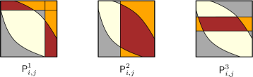
Figure 7: Examples of the approximate reachable free space in one cell: reachable by lower or left boundary (left), by a vertical tunnel (center), or a diagonal tunnel (right). (This figure is not referenced)

4.2.5 Computation of the gates

The gates of ${\mathsf{P}}_{i,j}$ can be computed in constant time. A gate of this set either lies on the grid of the parametric space, or it may be internal to the free space cell. The endpoints of a free space interval can be computed using the intersection of the corresponding edge and a disk of radius $\delta$ centered at the corresponding vertex. Internal gates of the free space can be computed in a similar way. One can use the Minkowski sum of the edge of $B$ with a disk of radius $\delta$. The intersection points of the resulting hippodrome with the edge of $T$ correspond to the $x$-coordinates of the gates, while we can obtain the $y$-coordinates by projecting the intersection point back onto the edge of $B$. A gate might also be the intersection point of a horizontal line with the free space as computed in Step 1 and Step 3 of the decision algorithm. Consider the diagonalTunnel procedure which we use to compute ${\mathsf{P}}^{3}_{i,j}$. The procedure computes a portion $\mathsf{u}$ of the edge $\mathsf{e}_{j}$ of $B$ by intersection with the line-stabbing wedge. In order to obtain the extremal points of the returned set in parametric space, we can take the Minkowski sum of $\mathsf{u}$ with a disk of radius $\delta$ and intersect the resulting hippodrome with the edge $\mathsf{e}_{i}$ of $T$. See Figure 8 for an illustration. We can a similar method for ${\mathsf{P}}^{1}_{i,j}$. The actual gates of ${\mathsf{P}}_{i,j}$ can then be computed using a simple case distinction.

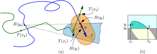
Figure 8: Computation of the gates $\mathsf{r}=(x_{\mathsf{r}},y_{\mathsf{r}})$ and $\mathsf{s}=(x_{\mathsf{s}},y_{\mathsf{s}})$ of ${\mathsf{P}}^{3}_{i,j}$.

4.3 Analysis

We now analyze the correctness and running time of the algorithm described above.

Lemma 4.2

Given a cell $C_{i,i}$, a point $\mathsf{p}\in\mathcal{D}_{\leq\delta}$ and a parameter $\delta\geq 0$, the diagonalTunnel procedure described in Section 4.2.3 returns a set of points ${\mathsf{P}}\subseteq C_{i,i}$, such that for any $\mathsf{q}\in C_{i,i}$, it holds that ${\mathrm{p{r}c}}_{\mathsf{\tau}}\!\left({\mathsf{p},\mathsf{q}}\right)\leq\delta$ if and only if $\mathsf{q}\in{\mathsf{P}}$.

Proof 4.3

The correctness of the procedure follows from the correctness of the line-stabbing algorithm as analyzed in [14]. Recall that we intersect the line-stabbing wedge of $B(y_{\mathsf{p}})$ and the disks $D_{1},\dots,D_{k}$ with the edge of $B$ that corresponds to $C_{i,i}$ to retrieve the horizontal slab in $C_{i,i}$ that defines ${\mathsf{P}}$. Refer to Figure 5 for an illustration. It follows that any directed line segment $\overline{B(y_{\mathsf{p}})B(y_{\mathsf{q}})}$, where $y_{\mathsf{q}}$ is the $y$-coordinate of a point $\mathsf{q}\in{\mathsf{P}}$, contains points $\mathsf{p}_{i}$ for $1\leq i\leq k$ in the order of $i$ along the segment, such that $\mathsf{p}_{i}\in D_{i}$. (For the case that $B(y_{\mathsf{p}})$ is contained in each of the disks $D_{1},\dots,D_{k}$, any line through $B(y_{\mathsf{p}})$ stabs the disks in any order, by choosing $\mathsf{p}_{i}=B(y_{\mathsf{p}})$ for all $1\leq i\leq k$.) Thus, we can match the shortcut $\overline{B}\!\left[\rule[0.0pt]{0.0pt}{9.95863pt}{y_{\mathsf{p}},y_{\mathsf{q}}}\right]$ to the subcurve ${T}\left[\rule[0.0pt]{0.0pt}{9.95863pt}{x_{\mathsf{p}},x_{\mathsf{q}}}\right]$ within Fréchet distance $\delta$ as follows. For any two inner vertices $\mathsf{v}_{i},\mathsf{v}_{i+1}$ of ${T}\left[\rule[0.0pt]{0.0pt}{9.95863pt}{x_{\mathsf{p}},x_{\mathsf{q}}}\right]$, we can match the edge connecting them to the line segment $\overline{\mathsf{p}_{i}\mathsf{p}_{i+1}}$ by Observation 4.1. For the first segment, note that we required $\mathsf{p}\in\mathcal{D}_{\leq\delta}$. For the last segment, we ensured that ${\mathsf{P}}\subseteq\mathcal{D}_{\leq\delta}$ by construction. Thus, also here we can apply Observation 4.1. As for the other direction, let $\mathsf{q}\in C_{i,i}$, such that ${\mathrm{p{r}c}}_{\mathsf{\tau}}\!\left({\mathsf{p},\mathsf{q}}\right)\leq\delta$. It must be, that the line segment from $B(y_{\mathsf{p}})$ to $B(y_{\mathsf{q}})$ stabs the disks $D_{1},\dots,D_{k}$ in the correct order. Thus, $B(y_{\mathsf{q}})$ would be included in the computed line-stabbing wedge and subsequently, $\mathsf{q}$ would be included in ${\mathsf{P}}$.

Lemma 4.4

For two polygonal curves $T$ and $B$ in ${\rm I\!R}^{2}$ of total complexity $n$, the diagonalTunnel procedure described in Section 4.2.3 takes $O(n\log n)$ time and $O(n)$ space.

Proof 4.5

Our modification of the line-stabbing algorithm does not increase the running time and space requirements of the algorithm, which is $O(k\log k)$ with $k$ being the number of disks handled. Intersecting the line-stabbing wedge with a line segment can be done in time $O(\log k)$, since the complexity of the wedge is $O(k)$. Thus, the claim follows directly from the analysis of the line-stabbing algorithm in [14] and by the fact that the algorithm handles at most $n$ disks.

Lemma 4.6

For any $1\leq i\leq n_{1}$ and $1\leq j\leq n_{2}$, let ${\mathsf{P}}^{3}_{i,j}$ be the set computed in Step 3 of the decision algorithm layed out in Figure 6 and let $R=\bigcup_{k=1}^{i-1}\bigcup_{\ell=1}^{i-1}{\mathsf{P}}_{k,\ell}$, i.e., the reachable points computed in the lower left quadrant of the cell. It holds that:

1. There exists a point $\mathsf{p}\in R$, such that for any $\mathsf{q}\in C_{i,j}$, the diagonal tunnel $\mathsf{\tau}\!\left({\mathsf{p},\mathsf{q}}\right)$ has price ${\mathrm{p{r}c}}_{\mathsf{\tau}}\!\left({\mathsf{p},\mathsf{q}}\right)\leq 3\delta$ if and only if $\mathsf{q}\in{\mathsf{P}}^{3}_{i,j}$.

2. There exists no other point $\mathsf{b}\in C_{i,j}\setminus{\mathsf{P}}^{3}_{i,j}$ that is the endpoint of a diagonal tunnel from $R$ with price at most $\delta$.

Proof 4.7

The lemma follows from the monotonicity of the tunnel prices, which is testified by Lemma 4.1 and from the correctness of the diagonalTunnel procedure (Lemma 4.2). Note that the algorithm computes the gates of $R$ within every cell. Furthermore, the gates are maintained in the arrays ${}\overline{g}^{r}$ and ${}g^{r}$, such that, when handling the cell $C_{i,j}$, we can retrieve the rightmost gate in the lower left quadrant of the lower left corner of $C_{i,j}$ from ${}\overline{g}^{r}[i-1]$. (This can be easily shown by induction on the cells in the order in which they are handled.) Let $\mathsf{p}$ be the point stored in ${}\overline{g}^{r}[i-1]$. Part (i) of the claim follows from Lemma 4.2, since diagonalTunnel is called with the parameter $\mathsf{p}$ to obtain ${\mathsf{P}}^{3}_{i,j}$. Part (ii) of the claim follows from Lemma 4.1, since $\mathsf{p}$ is the rightmost point in $R$ that could serve as a starting point for a diagonal tunnel ending in $C_{i,j}$. Indeed, assume that there would exist such points $\mathsf{b}\in C_{i,j}\setminus{\mathsf{P}}^{3}_{i,j}$ and $\mathsf{c}\in R$ with tunnel price ${\mathrm{p{r}c}}_{\mathsf{\tau}}\!\left({\mathsf{c},\mathsf{b}}\right)\leq\delta$. It must be that $\mathsf{b}$ lies to the left of $\mathsf{p}$, since $\mathsf{p}$ was the rightmost possible gate. By (i), ${\mathrm{p{r}c}}_{\mathsf{\tau}}\!\left({\mathsf{p},\mathsf{b}}\right)>3\delta$ and therefore Lemma 4.1 implies that ${\mathrm{p{r}c}}_{\mathsf{\tau}}\!\left({\mathsf{c},\mathsf{b}}\right)>\delta$, a contradiction.

Lemma 4.8

For any $1\leq i\leq n_{1}$ and $1\leq j\leq n_{2}$, let ${\mathsf{P}}^{2}_{i,j}$ be the set computed in Step 2 of the decision algorithm layed out in Figure 6. and let $R=\bigcup_{\ell=1}^{j-1}{\mathsf{P}}_{i,\ell}$, i.e., the reachable points computed in column $i$ below the cell. For any $\mathsf{q}\in C_{i,j}$, the vertical tunnel $\mathsf{\tau}\!\left({\mathsf{p},\mathsf{q}}\right)$ has price ${\mathrm{p{r}c}}_{\mathsf{\tau}}\!\left({\mathsf{p},\mathsf{q}}\right)\leq\delta$ for some $\mathsf{p}\in R$ if and only if $\mathsf{q}\in{\mathsf{P}}^{2}_{i,j}$.

Proof 4.9

Note that vertical tunnels are always affordable if they are feasible by Observation 4.1. As in the proof of Lemma 4.6, we note that the algorithm computes the gates of $R$ within every cell. Furthermore, gates are maintained in the arrays ${}\overline{g}^{\ell}$ and ${}g^{\ell}$, such that, when handling the cell $C_{i,j}$, we can retrieve the leftmost gate below $C_{i,j}$ in the same column from ${}\overline{g}^{\ell}[i]$. (Again, this can be easily shown by induction on the cells in the order in which they are handled.) Let $\mathsf{p}$ be the point stored in ${}\overline{g}^{\ell}[i]$ when handling the cell $C_{i,j}$. Since ${\mathsf{P}}^{2}_{i,j}$ is computed by calling verticalTunnel on $\mathsf{p}$, the claim follows.

Lemma 4.10

The output of the decision algorithm layed out in Figure 6 and described in Section 4.2.4 is correct.

Proof 4.11

The proof goes by induction on the order of the handled cells. We claim that for any point $\mathsf{q}\in C_{i,j}$ it holds that (a) if $\mathsf{q}\in{\mathsf{P}}_{i,j}$, then $\mathsf{q}\in\mathcal{R}_{\leq 3\delta}$, and (b) if $\mathsf{q}\in\mathcal{R}_{\leq\delta}$ then $\mathsf{q}\in{\mathsf{P}}_{i,j}$. For the first cell $C_{1,1}$, this is clearly true. Indeed, a shortcut from $B(0)$ to any point on the first edge of $B$, results in a shortcut curve that has Fréchet distance zero to $B$. By the convexity of the free space in a single cell, it follows that $\mathcal{R}_{\leq\delta}^{(1,1)}=\mathcal{D}_{\leq\delta}^{(1,1)}={\mathsf{P}}_{1,1}\subseteq\mathcal{R}_{\leq 3\delta}^{(1,1)}$ given that $(0,0)\in\mathcal{D}_{\leq\delta}$.

Now, consider a cell $C_{i,j}$ that is handled by the algorithm. We argue that part (a) of the induction hypothesis holds. It must be that either (i) $\mathsf{q}\in{\mathsf{P}}^{1}_{i,j}$, (ii) $\mathsf{q}\in{\mathsf{P}}^{2}_{i,j}$, (iii) $\mathsf{q}\in{\mathsf{P}}^{3}_{i,j}$, or (iv) $\mathsf{q}$ is in the upper right quadrant of some point $\mathsf{q}^{\prime}$ in one of ${\mathsf{P}}^{1}_{i,j},{\mathsf{P}}^{2}_{i,j}$ or ${\mathsf{P}}^{3}_{i,j}$. In cases (i), the claim follows by induction since ${\mathsf{P}}_{i-1,j}$ and ${\mathsf{P}}_{i,j-1}$ are computed before ${\mathsf{P}}_{i,j}$. In case (ii) the claim follows by induction, since the rows are handled from bottom to top and by Lemma 4.8. In case (iii) the claim follows by Lemma 4.6 and by induction, since the algorithm traverses the free space diagram in a row-by-row manner from bottom to top and in every row from left to right. Now, in case (iv), the claim follows from (i),(ii), or (iii). Indeed, we can always connect $\mathsf{q}^{\prime}$ with $\mathsf{q}$ by a straight line segment, and since $\mathcal{D}_{\leq\delta}$ is convex inside any cell, these straight monotone paths are preserved in the intersection with the free space.

It remains to prove part (b). Let $\mathsf{q}\in C_{i,j}$ be the endpoint of a monotone path from $(0,0)$ that stays inside the $\delta$-free space and otherwise uses tunnels of price at most $\delta$. There are three possibilities for $\pi$ to enter $C_{i,j}$: (i) via the boundary with its direct neighbors, (ii) via a vertical tunnel, or (iii) via a diagonal tunnel. (As for horizontal tunnels, we can always replace such a horizontal tunnel by the corresponding monotone path through the free space.) We can show in each of these cases that $\mathsf{q}$ should be included ${\mathsf{P}}_{i,j}$. In case (i) we can apply the induction hypothesis for ${\mathsf{P}}_{i-1,j}$ and ${\mathsf{P}}_{i,j-1}$, in case (ii) we can apply Lemma 4.8 and the induction hypothesis for cells below ${\mathsf{P}}_{i,j}$ in the same column and in case (iii) we can apply Lemma 4.6 and the induction hypothesis for cells in the lower left quadrant of the cell.

Lemma 4.12

Given two polygonal curves $T$ and $B$ in ${\rm I\!R}^{2}$ of complexity $n=n_{1}+n_{2}$, the decision algorithm takes time in $O(n^{3}\log n)$ and space in $O(n)$.

Proof 4.13

The algorithm keeps six arrays of length $n_{1}$, which store objects of constant complexity. The tunnel procedure takes space in $O(n)$, by Lemma 4.4. Thus, overall, the algorithm requires $O(n)$ space. As for the running time, the algorithm handles $O(n^{2})$ cells. Each cell is handled in three steps of which the first and second step take constant time each and the third step takes time in $O(n\log n)$ by Lemma 4.4. The computation of the gates can be done in constant time per cell. Furthermore, the algorithm takes $O(n)$ time per row to update the arrays. Overall, the running time can be bounded by $O(n^{3}\log n)$ time.

Theorem 4.14

Given two curves $T$ and $B$ of complexity $n=n_{1}+n_{2}$ and a value of $\delta$, the decision algorithm outputs one of the following, either

1. $d_{\mathcal{S}}\!\left({T,B}\right)\leq 3\delta$, or

2. $d_{\mathcal{S}}\!\left({T,B}\right)>\delta$.

In any case, the output is correct. The algorithm runs in $O(n^{3}\log n)$ time and $O(n)$ space.

4.4 Exact decision algorithm for vertex-restricted case

A similar strategy as the approximation algorithm for the general case gives an exact algorithm for deciding the vertex-restricted case. That is, given two polygonal curves $T,B$, and $\delta>0$, we want to decide whether $\mathsf{d}_{\mathcal{S}}\!\left({T,B}\right)\leq\delta$. For this, we again traverse the free space, and in each cell compute, additionally to the reachable free space from neighboring cells, the free space reachable using shortcuts between vertices. We observe that in the vertex-restricted case, tunnels can start and end only on grid lines, and hence the free space does not fragment. In the following, we assume that shortcuts may be taken on the curve corresponding to the vertical axis of the free space diagram, i.e., between horizontal grid lines.

Now, in each cell, instead of testing the shortest tunnel (as in the approximation algorithm), we need to test all tunnels between the upper horizontal cell boundary and (at most $n^{2}$) horizontal cell boundaries left and below the current cell. In fact, by the following lemma, (which is similar to the monotonicity of the prices of tunnels) we only need to test each shortcut with the shortest possible subcurve of the other curve. Thus, we only need to test $n$ tunnels.

Lemma 4.15

Let $\overline{B}=qq^{\prime}$ be a segment, and let ${T}_{2}$ be a subcurve of ${T}_{1}$, s.t. the start and end points of ${T}_{2}$ have distance at most $\delta$ to $q$ and $q^{\prime}$, respectively. Then it holds $\mathsf{d}_{\mathcal{F}}\!\left({{T}_{1},\overline{B}}\right)\leq\delta\Rightarrow\mathsf{d}_{\mathcal{F}}\!\left({{T}_{2},\overline{B}}\right)\leq\delta$.

Proof 4.16

Let $\sigma$ be a homeomorphism realizing a distance $\delta\geq\delta$ between $\overline{B}$ to ${T}_{1}$. We can easily modify $\sigma$ to a homeomorphism $\sigma^{\prime}$ realizing at most the same distance $\delta$ between $\overline{B}$ to ${T}_{2}$, as illustrated in the Figure.

Now, assume we are handling free space cell $C_{ij}$. First, we compute reachability from neighboring cells, as usual. Next we consider reachability by tunnels. The lemma above implies, that for each of the $j-1$ possible shortcuts (starting at $q_{h}<q_{j}$ and ending at $q_{j}$), we only need to test the tunnel corresponding to the shortest possible subcurve on $T$, i.e., starting at the rightmost point on $T$. If this tunnel has a price larger than $\delta$, then by the lemma so do all other tunnels starting at $p_{l}^{\prime}<p_{l}$. If this tunnel has price at most $\delta$, then the complete upper cell boundary is reachable and we do not need to test further tunnels. Thus, for all $h<j$ we test whether the tunnel from the rightmost point $p_{l}$ to the leftmost point $p_{k}$ on the current upper cell boundary has price $\leq\delta$. For this, we maintain for each vertex $q_{h}$ on $B$ the rightmost point $p_{l}$ on $T$ such that $(p_{l},q_{h})$ is in reachable free space. This can be updated in constant time per cell, and linear space in total. To test all $l-1$ possible tunnels per cell, we use a similar strategy as for the approximation algorithm in the previous section. We build the line stabbing wedge, from “left to right”, i.e., starting at $q_{j}$, and adding disks $p_{i},p_{i-1},\ldots$ For each $h<j$ we test if $q_{h}$ is in the wedge for the corresponding $p_{l}$.

The modified tunnel procedure for cell $C_{ij}$ takes $O(i\log i)$ time for computing the line-stabbing wedge and $O(j)$ time for testing tunnels, giving $O(i\log i+j)=O(n\log n)$ time in total. Thus, we can handle the complete free space diagram in $O(n^{3}\log n)$ time.

The correctness and runtime analysis of the algorithm follow in the lines of the approximation algorithm. We conclude with the following theorem.

Theorem 4.17

Given two curves $T$ and $B$ and a value of $\delta$. One can decide whether the vertex-restricted shortcut Fréchet distance between $T$ and $B$ is $\leq\delta$ in $O(n^{3}\log n)$ time and $O(n)$ space.

5 Conclusions

In this paper we studied the computational complexity of the shortcut Fréchet distance, that is the minimal Fréchet distance achieved by allowing shortcuts on one of two polygonal curves. We proved that this problem is NP-hard and doing so, provided the first NP-hardness result for a variant of the Fréchet distance between two polygonal curves in the plane. Furthermore, we gave polynomial time algorithms for the decision problem: an approximation algorithm for the general case and an exact algorithm for the vertex-restricted case, which improves upon a previous result.

Computation problem

An important open question is how to compute (or even approximate) the shortcut Fréchet distance. The standard way to compute the Fréchet distance is to use a decision procedure in a binary search over candidate values, also called critical values. These are determined by local geometric configurations such as the distance between a vertex and an edge [3]. Also for the vertex-restricted shortcut Fréchet distance, there are at most a polynomial number of critical values that need to be considered in the search [12]. The situation becomes more intricate in the general case where shortcuts are not confined to input vertices. In the example depicted in Figure 9, the shortcut Fréchet distance coincides with the minimum value of $\delta$ such that three tunnels can be connected monotonically along the base curve. The realizing shortcut curve is also shown. For any input size one can construct an example of this type where the critical value depends on the geometric configuration of a linear-size subset of edges. Thus, in order to compute all critical values of this type one would have to consider an exponential number of geometric configurations. A full characterization of the events and algorithms to compute or approximate the critical values is subject for further research.

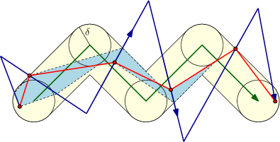
Figure 9: Example of a geometric configuration that determines the shortcut Fréchet distance.

In the light of these considerations it is interesting how the continuous and the vertex-restricted variant of the computation problem relate to each other. We can approximate the continuous variant (with additive error) by increasing the sampling of the input curve and using the vertex-restricted exact algorithm on the resulting curves. Thus, we can get arbitrarily close to the correct distance value for the continuous case by using a pseudo-polynomial algorithm. However, it is unclear if this helps in finding an exact solution for the continuous case.

[r] Note that there may be many combinatorially different shortcut curves which are close to the target curve under the Fréchet distance, as demonstrated by the example depicted in the figure to the right.

Complexity under restrictions

The base curve in our NP-hardness reduction self-intersects and is not $c$-packed. In fact, it cannot be $c$-packed for any placement of the connector edges for any constant $c$. 0 Whether the problem is NP-hard or polynomial time computable for $c$-packed, non-intersecting, or even monotone curves is currently unclear. Our reduction from SUBSET-SUM proves that the problem is weakly NP-hard. It would be interesting to determine whether it is also strongly NP-hard.

Shortcuts on both curves

We studied the shortcut Fréchet distance where shortcuts are only allowed on one curve. In [11] this is called the directed variant of the shortcut Fréchet distance. As we discussed in the introduction, this variant is important in applications. However, it may also be interesting to consider undirected (or symmetric) variants of the shortcut Fréchet problem, where shortcuts are allowed on either or both curves. The first question is how to define an undirected variant: One needs to restrict the set of eligible shortcuts, otherwise the minimization would be achieved by simply shortcutting both curves from start to end, and this does not yield a meaningful distance measure. A reasonable restriction could be to disallow shortcuts to be matched to each other under the Fréchet distance. Note that for this definition of the undirected shortcut Fréchet distance the presented NP-hardness proof also applies. Intuitively, shortcuts can only affect the target curve by either shortening or eliminating one or more twists. However, any feasible shortcut curve of the base curve has to pass through the buffer zones corresponding to these twists by using a shortcut. As a result, any shortcut on the target curve has to be matched at least partially to a shortcut of the base curve in order to affect the feasible solutions and this is prevented by definition.

Other variants

Another interesting direction of research would be to study the computational complexity of a discrete shortcut Fréchet distance. The discrete Fréchet distance only considers matchings between the vertices of the curves and can be computed using dynamic programming. In practice, such a discrete shortcut Fréchet distance might approximate the continuous version and it might be easier to compute. Thus it deserves further attention. Finally, it would also be interesting to study a weak shortcut Fréchet distance, where the reparameterizations not need be monotone. Again, one would first have to find a reasonable definition for this variant, and then study its computational complexity.

Acknowledgements

We thank Maarten Löffler for insightful discussions on the NP-hardness construction, and Sariel Har-Peled and anonymous referees for many helpful comments.

References

- [1] P. K. Agarwal, S. Har-Peled, N. H. Mustafa, and Y. Wang. Near-linear time approximation algorithms for curve simplification. Algorithmica, 42:203–219, 2005.
- [2] H. Alt, A. Efrat, G. Rote, and C. Wenk. Matching planar maps. Journal of Algorithms, 49:262–283, 2003.
- [3] H. Alt and M. Godau. Computing the Fréchet distance between two polygonal curves. International Journal of Computational Geometry & Applications, 5:75–91, 1995.
- [4] S. Bereg, M. Jiang, W. Wang, B. Yang, and B. Zhu. Simplifying 3d polygonal chains under the discrete Fréchet distance. In Proc. 8th Latin American Conference on Theoretical Informatics, pages 630–641, 2008.
- [5] S. Brakatsoulas, D. Pfoser, R. Salas, and C. Wenk. On map-matching vehicle tracking data. In Proc. 31st International Conference on Very Large Data Bases, pages 853–864, 2005.
- [6] K. Buchin, M. Buchin, and J. Gudmundsson. Detecting single file movement. In Proc. 16th ACM International Conference on Advances in Geographic Information Systems, pages 288–297, 2008.
- [7] K. Buchin, M. Buchin, J. Gudmundsson, M. Löffler, and J. Luo. Detecting commuting patterns by clustering subtrajectories. International Journal of Computational Geometry & Applications, 21(03):253–282, 2011.
- [8] K. Buchin, M. Buchin, W. Meulemans, and W. Mulzer. Four Soviets walk the dog—with an application to Alt’s conjecture. arXiv/1209.4403, 2012.
- [9] K. Buchin, M. Buchin, and Y. Wang. Exact algorithm for partial curve matching via the Fréchet distance. In Proc. 20th ACM-SIAM Symposium on Discrete Algorithms, pages 645–654, 2009.
- [10] M. de Berg and M. Streppel. Approximate range searching using binary space partitions. Computational Geometry: Theory and Applications, 33(3):139 – 151, 2006.
- [11] A. Driemel. Realistic Analysis for Algorithmic Problems on Geographical Data. PhD thesis, Utrecht University, 2013.
- [12] A. Driemel and S. Har-Peled. Jaywalking your dog – computing the Fréchet distance with shortcuts. SIAM Journal of Computing, 2013. To appear.
- [13] A. Driemel, S. Har-Peled, and C. Wenk. Approximating the fréchet distance for realistic curves in near linear time. Discrete & Computational Geometry, 48(1):94–127, 2012.
- [14] L. J. Guibas, J. Hershberger, J. S. B. Mitchell, and J. Snoeyink. Approximating polygons and subdivisions with minimum link paths. In Proc. 2nd International Symposium on Algorithms, pages 151–162, 1991.
- [15] A. Mascret, T. Devogele, I. L. Berre, and A. Hénaff. Coastline matching process based on the discrete Fréchet distance. In Proc. 12th International Symposium on Spatial Data Handling, pages 383–400, 2006.
- [16] T. Wylie and B. Zhu. A polynomial time solution for protein chain pair simplification under the discrete Fréchet distance. In Proc. 8th International Symposium on Bioinformatics Research and Applications, volume 7292 of Lecture Notes in Computer Science, pages 287–298, 2012.