A new construction of Lagrangians
in the complex Euclidean plane
in terms of planar curves

Abstract.

We introduce a new method to construct a large family of Lagrangian surfaces in complex Euclidean plane $\mathbb{C}^{2}$ by means of two planar curves making use of their usual product as complex functions and integrating the Hermitian product of their position and tangent vectors.

Among this family, we characterize minimal, constant mean curvature, Hamiltonian stationary, solitons for mean curvature flow and Willmore surfaces in terms of simple properties of the curvatures of the generating curves. As an application, we provide explicitly conformal parametrizations of known and new examples of these classes of Lagrangians in $\mathbb{C}^{2}$.

1. Introduction

An isometric immersion $\phi:M^{n}\rightarrow\widetilde{M}^{n}$ of an $n$-dimensional Riemannian manifold $M^{n}$ into an $n$-dimensional Kaehler manifold $\widetilde{M}^{n}$ is said to be Lagrangian if the complex structure $J$ of $\widetilde{M}^{n}$ interchanges each tangent space of $M^{n}$ with its corresponding normal space. Lagrangian submanifolds appear naturally in several contexts of Mathematical Physics. For example, special Lagrangian submanifolds of the complex Euclidean space $\mathbb{C}^{n}$ (or of a Calabi-Yau manifold) have been studied widely and in [18] it was proposed an explanation of mirror symmetry in terms of the moduli spaces of special Lagrangian submanifolds. These submanifolds are volume minimizing and, in particular, they are minimal submanifolds. In the two-dimensional case, special Lagrangian surfaces of $\mathbb{C}^{2}$ are exactly complex surfaces with respect to another complex structure on $\mathbb{R}^{4}\equiv\mathbb{C}^{2}$.

The simplest examples of Lagrangian surfaces in $\mathbb{C}^{2}$ are given by the product of two planar curves $\alpha=\alpha(t)$, $t\in I_{1}\subseteq\mathbb{R}$, and $\omega=\omega(s)$, $s\in I_{2}\subseteq\mathbb{R}$:

(1.1) $$(t,s)\stackrel{{\scriptstyle\phi}}{{\longmapsto}}\left(\alpha(t),\omega(s)\right).$$

Another fruitful method of construction of Lagrangian surfaces in $\mathbb{C}^{2}$ is obtained when one takes the particular version for the two-dimensional case of Proposition 3 in [16] (see also [7] and [2]), involving a planar curve $\alpha=\alpha(t)$, $t\in I_{1}\subseteq\mathbb{R}$, and a Legendre curve $(\gamma_{1},\gamma_{2})=\gamma=\gamma(s)$, $s\in I_{2}\subseteq\mathbb{R}$, in the 3-sphere $\mathbb{S}^{3}\subset\mathbb{C}^{2}$

(1.2) $$(t,s)\stackrel{{\scriptstyle\phi}}{{\longmapsto}}\alpha(t)\cdot\gamma(s)=\alpha(t)\left(\gamma_{1}(s),\gamma_{2}(s)\right).$$

In [4], it was presented a different method to construct a large family of Lagrangian surfaces in $\mathbb{C}^{2}$ using a Legendre curve $(\alpha_{1},\alpha_{2})=\alpha(t)$, $t\in I_{1}\subseteq\mathbb{R}$, in the anti De Sitter 3-space $\mathbb{H}^{3}_{1}\subset\mathbb{C}^{2}$ and a Legendre curve $(\gamma_{1},\gamma_{2})=\gamma(s)$, $s\in I_{2}\subseteq\mathbb{R}$, in $\mathbb{S}^{3}\subset\mathbb{C}^{2}$:

(1.3) $$(t,s)\stackrel{{\scriptstyle\phi}}{{\longmapsto}}\left(\alpha_{1}(t)\gamma_{1}(s),\alpha_{2}(t)\gamma_{2}(s)\right).$$

We observe that in the constructions (1.1), (1.2) and (1.3) the components of the position vector $\phi=(\phi_{1},\phi_{2})$ of the immersions are given by the product of two complex functions:

(1.4) $$\phi_{1}(t,s)=\begin{cases}\alpha(t)\\ \alpha(t)\gamma_{1}(s)\\ \alpha_{1}(t)\gamma_{1}(s)\end{cases},\qquad\phi_{2}(t,s)\begin{cases}\omega(s)\\ \alpha(t)\gamma_{2}(s)\\ \alpha_{2}(t)\gamma_{2}(s)\end{cases}.$$

From an algebraic point of view, we propose now to consider one of the components as a product of two complex functions and the other as an addition of another two complex functions. So, we can consider the following type of possible Lagrangian immersions:

(1.5) $$\phi(t,s)=\left(f(t)+g(s),\alpha(t)\omega(s)\right),$$

where $\alpha=\alpha(t)$, $t\in I_{1}\subseteq\mathbb{R}$ and $\omega=\omega(s)$, $s\in I_{2}\subseteq\mathbb{R}$ are planar curves. If we impose that $\phi$ gives an orthonormal parametrization of a Lagrangian immersion, we have that $\left(\phi_{t},\phi_{s}\right)=0$, where $(\cdot,\cdot)$ denotes the usual bilinear Hermitian product of $\mathbb{C}^{2}$. Since $\phi_{t}=(f^{\prime}(t),\alpha^{\prime}(t)\omega(s))$ and $\phi_{s}=(\dot{g}(s),\alpha(t)\dot{\omega}(s))$ where ^′ (resp. $\dot{\ }$) means derivate respect to $t$ (resp. to $s$), we get

(1.6) $$f^{\prime}(t)\overline{\dot{g}(s)}+\alpha^{\prime}(t)\overline{\alpha(t)}\omega(s)\overline{\dot{\omega}(s)}=0.$$

So, essentially we can take

(1.7) $$f(t)=-\int\alpha^{\prime}(t)\overline{\alpha(t)}dt,\qquad g(s)=\int\dot{\omega}(s)\overline{\omega(s)}ds.$$

Putting this in (1.5) we can check that

(1.8) $$\phi(t,s)=\left(\int\dot{\omega}(s)\overline{\omega(s)}ds-\int\alpha^{\prime}(t)\overline{\alpha(t)}dt,\alpha(t)\omega(s)\right)$$

is a Lagrangian immersion constructed from two planar curves (see Theorem 2.1), well defined up to a translation in $\mathbb{C}^{2}$.

An interesting problem in this setting is to find nontrivial examples of Lagrangian surfaces with some given geometric properties. In this paper we pay our attention to an extrinsic point of view and focus on several classical equations involving the mean curvature vector and natural associated variational problems. In this way, we determine in our construction of Lagrangians not only those which are minimal, have parallel mean curvature vector or constant mean curvature, but also those ones that are Hamiltonian stationary, solitons of mean curvature flow or Willmore.

When we involve lines and circles in (1.8) we get the most regular surfaces: special Lagrangians (Corollary 3.1) and Hamiltonian stationary Lagrangians (Corollary 3.3). In this setting, we provide explicit conformal parametrizations of some known examples in terms of elementary functions and obtain some new examples of interesting Hamiltonian stationary Lagrangians. With some more sophisticated curves, we obtain a very large family of new Lagrangians with constant mean curvature vector (Corollary 3.4), which includes a (branched) Lagrangian torus. Our construction (1.8) is actually inspired in the Lagrangian translating solitons obtained in [6] associated to certain special solutions of the curve shortening flow that we recover in Corollary 3.6. We also provide Willmore Lagrangians when we consider free elastic curves (Corollary 3.7). Finally, we illustrate in section 3.8 that we can also arrive at Lagrangian tori starting from certain closed curves.

The key point of the proof of all our results is the simple expression (2.5) for the mean curvature vector of the Lagrangian immersion in terms of the curvature functions of the generatrix curves.

2. The construction

In the complex Euclidean plane $\mathbb{C}^{2}$ we consider the bilinear Hermitian product defined by

$$(z,w)=z_{1}\bar{w}_{1}+z_{2}\bar{w}_{2},\quad z,w\in\mathbb{C}^{2}.$$

Then $\langle\,\,,\,\rangle={\rm Re}(\,\,,\,)$ is the Euclidean metric on $\mathbb{C}^{2}$ and $\omega=-{\rm Im}(\,,)$ is the Kaehler two-form given by $\omega(\,\cdot\,,\,\cdot\,)=\langle J\cdot,\cdot\rangle$, where $J$ is the complex structure on $\mathbb{C}^{2}$.

Let $\phi:M\rightarrow\mathbb{C}^{2}$ be an isometric immersion of a surface $M$ into $\mathbb{C}^{2}$. $\phi$ is said to be Lagrangian if $\phi^{*}\omega=0$. Then we have $\phi^{*}T\mathbb{C}^{2}=\phi_{*}TM\oplus J\phi_{*}TM$, where $TM$ is the tangent bundle of $M$. The second fundamental form $\sigma$ of $\phi$ is given by $\sigma(v,w)=JA_{Jv}w$, where $A$ is the shape operator, and so the trilinear form

$$C(\cdot,\cdot,\cdot)=\langle\sigma(\cdot,\cdot),J\cdot\rangle$$

is fully symmetric.

Suppose $M$ is orientable and let $\omega_{M}$ be the area form of $M$. If $\Omega=dz_{1}\wedge dz_{2}$ is the closed complex-valued 2-form of $\mathbb{C}^{2}$, then $\phi^{*}\Omega=e^{i\beta}\omega_{M}$, where $\beta:M\rightarrow\mathbb{R}/2\pi\mathbb{Z}$ is called the Lagrangian angle map of $\phi$ (see [11]). In general, $\beta$ is a multivalued function; nevertheless $d\beta$ is a well defined closed 1-form on $M$ and its cohomology class is called the Maslov class.

It is remarkable that $\beta$ satisfies (see for example [17])

(2.1) $$H=J\nabla\beta,$$

where $H$ is the mean curvature vector of $\phi$, defined by $H={\rm trace}\,\sigma$.

In this section, we describe a new method to contruct Lagrangian surfaces in complex Euclidean plane $\mathbb{C}^{2}$ with nice geometric properties, in the sense of they are similar to those of a product of curves.

Theorem 2.1.

Let $\alpha=\alpha(t)\subset\mathbb{C}\setminus\{0\}$, $t\in I_{1}$, and $\omega=\omega(s)\subset\mathbb{C}\setminus\{0\}$, $s\in I_{2}$, be regular planar curves, where $I_{1}$ and $I_{2}$ are intervals of $\mathbb{R}$. For any $t_{0}\in I_{1}$ and $s_{0}\in I_{2}$, let define

$$\Phi=\alpha\ast\omega:I_{1}\times I_{2}\subset\mathbb{R}^{2}\rightarrow\mathbb{C}^{2}=\mathbb{C}\times\mathbb{C}$$

$$\Phi(t,s)=\left(\int_{s_{0}}^{s}\dot{\omega}(y)\overline{\omega(y)}dy-\int_{t_{0}}^{t}\alpha^{\prime}(x)\overline{\alpha(x)}dx\,,\,\alpha(t)\omega(s)\right).$$

Then $\Phi$ is a Lagrangian immersion whose induced metric is

(2.2) $$\Phi^{*}\langle\ ,\ \rangle=\left(|\alpha|^{2}+|\omega|^{2}\right)\left(|\alpha^{\prime}|^{2}dt^{2}+|\dot{\omega}|^{2}ds^{2}\right),$$

where ^′ and ^⋅ denote the derivatives respect to $t$ and $s$ respectively.

The intrinsic tensor $C(\cdot,\cdot,\cdot)=\langle\sigma(\cdot,\cdot),J\cdot\rangle$ of $\Phi=\alpha\ast\omega$ is given by

(2.3) $$C(\partial_{t},\partial_{t},\partial_{t}) =|\alpha^{\prime}|^{2}\left((|\alpha|^{2}+|\omega|^{2})|\alpha^{\prime}|\kappa_{\alpha}-\langle\alpha^{\prime},J\alpha\rangle\right)$$

$$C(\partial_{t},\partial_{t},\partial_{s}) =|\alpha^{\prime}|^{2}\langle\dot{\omega},J\omega\rangle$$

$$C(\partial_{t},\partial_{s},\partial_{s}) =|\dot{\omega}|^{2}\langle\alpha^{\prime},J\alpha\rangle$$

$$C(\partial_{s},\partial_{s},\partial_{s}) =|\dot{\omega}|^{2}\left((|\alpha|^{2}+|\omega|^{2})|\dot{\omega}|\kappa_{\omega}-\langle\dot{\omega},J\omega\rangle\right)$$

where $\kappa_{\alpha}$ and $\kappa_{\omega}$ are the curvature functions of $\alpha$ and $\omega$, and $J$ also denotes the $+\pi/2$-rotation acting on $\mathbb{C}\equiv\mathbb{R}^{2}$.

The Lagrangian angle map of $\Phi=\alpha\ast\omega$ is given by

(2.4) $$\beta=\arg\left(\alpha^{\prime}\right)+\arg\left(\dot{\omega}\right)+\pi$$

and the mean curvature vector $H$ of $\Phi=\alpha\ast\omega$ by

(2.5) $$H=\frac{1}{|\alpha|^{2}+|\omega|^{2}}\left(\frac{\kappa_{\alpha}}{|\alpha^{\prime}|}J\Phi_{t}+\frac{\kappa_{\omega}}{|\dot{\omega}|}J\Phi_{s}\right).$$

Proof.

We first compute the tangent vector fields

$$\Phi_{t}=\alpha^{\prime}\left(-\overline{\alpha},\omega\right),\qquad\Phi_{s}=\dot{\omega}\left(\overline{\omega},\alpha\right).$$

Then we obtain $|\Phi_{t}|^{2}=|\alpha^{\prime}|^{2}\left(|\alpha|^{2}+|\omega|^{2}\right)$, $|\Phi_{s}|^{2}=|\dot{\omega}|^{2}\left(|\alpha|^{2}+|\omega|^{2}\right)$ and $\left(\Phi_{t},\Phi_{s}\right)=0$. So $\Phi$ is a Lagrangian immersion whose induced metric is written as in (2.2).

Taking imaginary parts in $(\Phi_{tt},\Phi_{t})$, $(\Phi_{tt},\Phi_{s})$, $(\Phi_{ss},\Phi_{t})$ and $(\Phi_{ss},\Phi_{s})$, we obtain the formulas given for the tensor $C$ in (2.3).

Using the definition of the Lagrangian angle map $\beta$, we obtain that

$$e^{i\beta}=\det_{\mathbb{C}}\Bigl{(}\frac{\Phi_{t}}{|\Phi_{t}|},\frac{\Phi_{s}}{|\Phi_{s}|}\Bigr{)}=-\frac{\alpha^{\prime}\dot{\omega}}{|\alpha^{\prime}||\dot{\omega}|}$$

and so we arrive at (2.4).

Finally, we can get the expresion (2.5) for $H$ using (2.1) taking into account that $\left(\arg\alpha^{\prime}\right)^{\prime}=|\alpha^{\prime}|\kappa_{\alpha}$ and $(\arg\dot{\omega})\dot{\ }=|\dot{\omega}|\kappa_{\omega}$, or directly from (2.3) using the orthonormal frame $\Bigl{\{}e_{1}=\frac{\partial_{t}}{|\alpha^{\prime}|\sqrt{|\alpha|^{2}+|\omega|^{2}}},\,e_{2}=\frac{\partial_{s}}{|\dot{\omega}|\sqrt{|\alpha|^{2}+|\omega|^{2}}}\Bigr{\}}$. ∎

Remark 2.1.

Up to a translation, we can rewrite the Lagrangian immersion $\Phi=\alpha\ast\omega$ as

$$\Phi(t,s)=\left(\frac{|\omega(s)|^{2}}{2}+\int_{s_{0}}^{s}\langle\dot{\omega},J\omega\rangle(y)dy-\frac{|\alpha(t)|^{2}}{2}-\int_{t_{0}}^{t}\ \langle\alpha^{\prime},J\alpha\rangle(x)dx\,,\,\alpha(t)\omega(s)\right).$$

From (2.2), we also observe that $\left(t^{*},s^{*}\right)\in I_{1}\times I_{2}$ is a singular point of $\Phi=\alpha\ast\omega$ if and only if $\alpha(t^{*})=0=\omega(s^{*})$.

Remark 2.2.

Interchanging the roles of $\alpha$ and $\omega$ is produced congruent Lagrangians in $\mathbb{C}^{2}$. In addition, the same happens with rotations of $\alpha$ and/or $\omega$. But only if we consider the same homotethy for $\alpha$ and $\omega$ we get homothetic Lagrangian immersions, concretely, $\rho\alpha\ast\rho\omega=\rho^{2}\alpha\ast\omega,\,\forall\rho>0$.

For example, the totally geodesic Lagrangian plane is recovered in our construction simply considering straight lines passing through the origin, $\alpha(t)=t$, $t\in\mathbb{R}$, $\omega(s)=s$, $s\in\mathbb{R}$, since in this case

(2.6) $$\left(\alpha\ast\omega\right)(t,s)=\left(\frac{s^{2}-t^{2}}{2},t\,s\right).$$

3. Applications

This section is devoted to study several families of Lagrangian surfaces in our construction described in Theorem 2.1; those characterized by different geometric properties related with the behavior of the mean curvature vector.

3.1. Special Lagrangians

A Lagrangian oriented surface is called special if its Lagrangian angle is constant ($\beta\equiv\beta_{0}$). From (2.1) this means that $H=0$, that is, the Lagrangian immersion is minimal, but in fact is area-minimizing because they are calibrated by ${\rm Re}(e^{-i\beta_{0}}\Omega)$ (see [11]). It is well known that these surfaces should be holomorphic curves with respect to another complex structure on $\mathbb{C}^{2}$.

Corollary 3.1.

The immersion $\Phi=\alpha\ast\omega$, given in Theorem 2.1, is special Lagrangian if and only if $\alpha$ and $\omega$ are straight lines.

Putting $\alpha(t)=t+i\,a$, $a\in\mathbb{R}$, and $\omega(s)=s+i\,b$, $b\in\mathbb{R}$, then $\Phi=\alpha\ast\omega$ can be written, up to a translation in $\mathbb{C}^{2}$, by

(3.1) $$\Phi(t,s)=\left(\frac{s^{2}-t^{2}}{2}+i(at-bs),ts+i(as+bt)\right),\ (t,s)\in\mathbb{R}^{2}.$$

If $(a,b)=(0,0)$, we get the totally geodesic Lagrangian plane (2.6). If $(a,b)\neq(0,0)$, these special Lagrangians correspond to the holomorphic curves $z\mapsto c\,z^{2}$, $c=-\frac{(a-ib)^{2}}{2(a^{2}+b^{2})^{2}}\in\mathbb{C}^{*}$.

Remark 3.1.

According to [13], the graphs $z\mapsto c\,z^{2},\,c>0$, are the only complete orientable minimal surfaces in Euclidean $n$-space with finite total curvature $-2\pi$. Topologically they are cylinders lying in $\mathbb{R}^{4}$ and (3.1) provides a conformal Lagrangian parametrization of them.

Proof.

From (2.5) we get that the minimality of $\Phi=\alpha\ast\omega$ is equivalent to $\kappa_{\alpha}=0=\kappa_{\omega}$. Then $\alpha$ and $\omega$ must be straight lines. So, up to rotations, we can consider $\alpha(t)=t+i\,a$, $a\in\mathbb{R}$, and $\omega(s)=s+i\,b$, $b\in\mathbb{R}$, and it is a straightforward computation to get (3.1).

If $(a,b)\neq(0,0)$, considering $\varphi:\mathbb{C}^{2}\rightarrow\mathbb{C}^{2}$, $\varphi(x_{1}+i\,y_{1},x_{2}+i\,y_{2})=(y_{1}+i\,y_{2},x_{1}-i\,x_{2})$ and $w=t+i\,s\in\mathbb{C}$, one easily obtains the holomorphic map

$$\left(\varphi\circ\Phi\right)(w)=\left((a+i\,b)\,w,-\frac{w^{2}}{2}\right)\subset\mathbb{C}^{2}.$$

Letting $w=(a+i\,b)\,z$, we finally get $\left(\varphi\circ\Phi\right)(z)=\Bigl{(}z,-\frac{(a-ib)^{2}}{2(a^{2}+b^{2})^{2}}\,z^{2}\Bigr{)}$ and the proof is finished. ∎

3.2. Lagrangians with parallel mean curvature vector

From the point of view of the mean curvature vector $H$, the easiest (non minimal) examples are those with parallel mean curvature vector, i.e., $\nabla^{\perp}H=0$, where $\nabla^{\perp}$ is the connection in the normal bundle. In the Lagrangian setting, the complex structure $J$ defines an isomorphism between the tangent and the normal bundles, so the condition to have parallel mean curvature vector is equivalent to the fact that $JH$ is a parallel vector field.

In the next result, we show that the right circular cylinder is the only Lagrangian with parallel mean curvature vector in our construction.

Corollary 3.2.

The Lagrangian immersion $\Phi=\alpha\ast\omega$, given in Theorem 2.1, has parallel (non null) mean curvature vector if and only if $\alpha$ and $\omega$ are both circles centered at the origin.

Putting $\alpha(t)=e^{it}$ and $\omega(s)=R\,e^{is}$, $R>0$, then $\Phi=\alpha\ast\omega$ can be written by

(3.2) $$\Phi(t,s)=\left(i(R^{2}s-t),R\,e^{i(s+t)}\right),\ (t,s)\in\mathbb{R}^{2}$$

that describes the right circular cylinder $\mathbb{R}\times\mathbb{S}^{1}(R)$.

Proof.

Without loss of generality we can consider $\alpha$ and $\omega$ curves parametrized by arclength. From (2.2) the induced metric is given by $e^{2u}\left(dt^{2}+ds^{2}\right)$, where $e^{2u}=|\alpha|^{2}+|\omega|^{2}$. Using (2.5), it is not difficult to check that $JH=-e^{-2u}(\kappa_{\alpha}\partial_{t}+\kappa_{\omega}\partial_{s})$ is a parallel vector field if and only if

(3.3) $$\kappa_{\alpha}^{\prime}-u_{t}\kappa_{\alpha}+u_{s}\kappa_{\omega}=0,\quad u_{t}\kappa_{\omega}+u_{s}\kappa_{\alpha}=0,\quad\dot{\kappa}_{\omega}-u_{s}\kappa_{\omega}+u_{t}\kappa_{\alpha}=0.$$

From the first and the third equation of (3.3) we deduce that $\kappa_{\alpha}^{\prime}+\dot{\kappa}_{\omega}=0$ and hence $\kappa_{\alpha}(t)=a\,t+b$ and $\kappa_{\omega}(s)=-a\,s+c$, with $a$, $b$, $c\in\mathbb{R}$. We distinguish three cases: We first suppose that $u_{s}=0$. It is equivalent to $|\omega|$ is constant. Using (3.3) and the fact that $\phi$ is non minimal, it follows that $u_{t}=0$ what means that $|\alpha|$ is also constant. If $u_{t}=0$ similarly we get that $|\alpha|$ and $|\omega|$ are constants. Finally, if $u_{t}\neq 0$ and $u_{s}\neq 0$, from the second equation of (3.3), there exists $c_{1}\in\mathbb{R}^{*}$ such that $\kappa_{\alpha}=c_{1}u_{t}$ and $\kappa_{\omega}=-c_{1}u_{s}$. So $u_{t}=(at+b)/c_{1}$ and $u_{s}=(as-c)/c_{1}$. Putting this information in (3.3), we arrive at $a=b=c=0$ which is a contradiction since we are assuming that $H\neq 0$. ∎

3.3. Hamiltonian stationary Lagrangians

A Lagrangian surface is called Hamiltonian stationary if the Lagrangian angle $\beta$ is harmonic, i.e. $\Delta\beta=0$, where $\Delta$ is the Laplace operator on $M$. Using (2.1), this is equivalent to the vanishing of the divergence of the tangent vector field $JH$. Hamiltonian stationary Lagrangian (in short HSL) surfaces are critical points of the area functional with respect to a special class of infinitesimal variations preserving the Lagrangian constraint; namely, the class of compactly supported Hamiltonian vector fields (see [15]). Special Lagrangians and Lagrangians with parallel mean curvature vector are trivial examples of HSL surfaces in $\mathbb{C}^{2}$; more interesting examples can be found in [1] [2], [8] and [12].

Corollary 3.3.

The immersion $\Phi=\alpha\ast\omega$, given in Theorem 2.1, is Hamiltonian stationary Lagrangian if and only if the curvature functions $k_{\alpha}$ and $k_{\omega}$ of $\alpha$ and $\omega$ are given by $k_{\alpha}(t)=at+b$ and $k_{\omega}(s)=-as+c$, with $a,b,c\in\mathbb{R}$, and where $t$ and $s$ are the arclength parameters of $\alpha$ and $\omega$, respectively.

Proof.

Without loss of generality we can consider $\alpha$ and $\omega$ parametrized by arclength and, in this way $\Phi$ is conformal. The Lagrangian surface $\Phi=\alpha\ast\omega$ is Hamiltonian stationary if and only if the Lagrangian angle map $\beta$ verifies $\Delta\beta=0$. So, using (2.4), we get that $\Phi$ is HSL if and only if the curvature functions $\kappa_{\alpha}$ and $\kappa_{\omega}$ of $\alpha$ and $\omega$ satisfy $\kappa_{\alpha}^{\prime}+\dot{\kappa}_{\omega}=0$, where ^′ and ^⋅ denote the derivatives respect to the arclength parameters $t$ and $s$, respectively. Then there exists $a\in\mathbb{R}$ such that $\kappa_{\alpha}^{\prime}=a=-\dot{\kappa}_{\omega}$ and this finishes the proof of the corollary. ∎

We distinguish two essential cases in the family described in Corollary 3.3:

Case 1: $a=0$, i.e. $\kappa_{\alpha}\equiv b$ and $\kappa_{\omega}\equiv c$. So, $\alpha$ and $\omega$ are either straight lines or circles. If $\alpha$ and $\omega$ are both straight lines we lie in the situation of Corollary 3.1 obtaining the special Lagrangians described there. Otherwise, we get the following subcases: either $b\neq 0$ and $c=0$ (or $b=0$ and $c\neq 0$) or $b\neq 0$ and $c\neq 0$.

First, if $b\neq 0$ and $c=0$, taking $\alpha(t)=a_{0}+R\,e^{it/R}$, with $R=1/|b|>0$, and $\omega(s)=s+i\,b_{0}$, $a_{0},b_{0}\geq 0$, then $\Phi=\alpha\ast\omega$ can be written, up to a translation in $\mathbb{C}^{2}$, by

$$\Phi(t,s)=\left(\frac{s^{2}}{2}-R\,a_{0}\,e^{it/R}-i(b_{0}\,s+Rt),a_{0}s+R(s+ib_{0})e^{it/R}\right),\,(t,s)\in\mathbb{R}^{2}.$$

In particular, when $a_{0}=b_{0}=0$, $R=1$ we get $(t,s)\mapsto\left(\frac{s^{2}}{2}-it,s\,e^{it}\right)$, which corresponds to the complete non-trivial HSL plane described in Corollary 3.5 of [6].

Second, if $b\neq 0$ and $c\neq 0$, up to a dilation we can consider $b=1$, $|c|=1/R$, and take $\alpha(t)=a_{1}+e^{it}$ and $\omega(s)=a_{2}+Re^{is/R}$, $a_{1},a_{2}\geq 0,\,R>0$. Then $\Phi=\alpha\ast\omega$ can be written, up to a translation in $\mathbb{C}^{2}$, by

$$\Phi(t,s)=\left(a_{2}Re^{is/R}\!-\!a_{1}e^{it}\!+\!i(Rs-t),a_{1}Re^{is/R}\!+\!a_{2}e^{it}\!+\!R\,e^{i(t+s/R)}\right),\,(t,s)\in\mathbb{R}^{2}.$$

In particular, when $a_{1}=a_{2}=0$ we recover the right circular cylinder $\mathbb{R}\times\mathbb{S}^{1}(R)$.

The above immersions provide conformal parametrizations of HSL complete surfaces, some of them studied in [1] from a different approach.

Case 2: $a\neq 0$, i.e. $\kappa_{\alpha}$ and $\kappa_{\omega}$ are certain linear functions of the arc parameter. After applying suitable translations on the parameter, we can consider $\kappa_{\alpha}(t)=a\,t$ and $\kappa_{\omega}(s)=-a\,s$. Thus, in this case $\alpha$ and $\omega$ must be Cornu spirals with opposite parameter. The corresponding immersions $\alpha\ast\omega$ provide new examples of HSL surfaces.

3.4. Lagrangians with constant mean curvature

A Lagrangian surface has constant mean curvature if $|H|$ is constant. Examples of Lagrangians with constant mean curvature can be found in [10]

Corollary 3.4.

The immersion $\Phi=\alpha\ast\omega$, given in Theorem 2.1, has constant mean curvature $|H|\equiv\rho>0$ if and only if the curvature functions $k_{\alpha}$ and $k_{\omega}$ of $\alpha$ and $\omega$ satisfy, respectively, $\kappa_{\alpha}^{2}=\rho^{2}|\alpha|^{2}-\lambda$ and $\kappa_{\omega}^{2}=\rho^{2}|\omega|^{2}+\lambda$, for some $\lambda\in\mathbb{R}$.

Proof.

Using the expresion (2.5), it follows that

$$|H|^{2}=\frac{1}{|\alpha|^{2}+|\omega|^{2}}\left(\kappa_{\alpha}^{2}+\kappa_{\omega}^{2}\right).$$

If $|H|\equiv\rho$, since $\alpha$ depends on $t$ and $\omega$ depends on $s$, there exists $\lambda\in\mathbb{R}$ such that $\kappa_{\omega}^{2}-\rho^{2}|\omega|^{2}=\lambda=\rho^{2}|\alpha|^{2}-\kappa_{\alpha}^{2}$, what proves the result. ∎

Now we show how the conditions on $\alpha$ and $\omega$ given in Corollary 3.4 determine both curves. If we take $\alpha$ and $\omega$ planar curves parametrized by arclength, they can be written as follows

$$\alpha =r_{1}\,e^{i\int\frac{\sqrt{1-r_{1}^{\prime 2}}}{r_{1}}},\quad r_{1}=r_{1}(t)=|\alpha(t)|,$$

$$\omega =r_{2}\,e^{i\int\frac{\sqrt{1-\dot{r}_{2}^{2}}}{r_{2}}},\quad r_{2}=r_{2}(s)=|\omega(s)|.$$

It is not difficult to check that the curvatures $\kappa_{\alpha}$ and $\kappa_{\omega}$ can be expressed in terms of the derivatives of $r_{1}$ and $r_{2}$ by the following equations:

$$r_{1}\sqrt{1-r_{1}^{\prime 2}}\,\kappa_{\alpha}=1-r_{1}^{\prime 2}-r_{1}r_{1}^{\prime\prime},\qquad r_{2}\sqrt{1-\dot{r}_{2}^{2}}\,\kappa_{\omega}=1-\dot{r}_{2}^{2}-r_{2}\ddot{r}_{2}.$$

Studying the case of Corollary 3.4, i.e. $\kappa_{\alpha}^{2}=\rho^{2}r_{1}^{2}-\lambda$ and $\kappa_{\omega}^{2}=\rho^{2}r_{2}^{2}+\lambda$, we get the following ordinary differential equations for $r_{1}$ and $r_{2}$:

(3.4) $$(1-r_{1}^{\prime 2}-r_{1}r_{1}^{\prime\prime})^{2}=\left(\rho^{2}r_{1}^{2}-\lambda\right)r_{1}^{2}(1-r_{1}^{\prime 2}),$$

(3.5) $$(1-\dot{r}_{2}^{2}-r_{2}\ddot{r}_{2})^{2}=\left(\rho^{2}r_{2}^{2}+\lambda\right)r_{2}^{2}(1-\dot{r}_{2}^{2}).$$

When we consider $r_{1}$ and $r_{2}$ constant, we recover the right circular cylinder obtained in the Corollary 3.2 corresponding to the parallel mean curvature case.

In the general case, we are able to obtain first integrals of the differential equations (3.4) and (3.5):

(3.6) $$\frac{\left(\rho^{2}r_{1}^{2}-\lambda\right)^{3/2}}{\rho^{2}}+\mu_{1}=3\,r_{1}\sqrt{1-r_{1}^{\prime 2}},$$

and

(3.7) $$\frac{\left(\rho^{2}r_{2}^{2}+\lambda\right)^{3/2}}{\rho^{2}}+\mu_{2}=3\,r_{2}\sqrt{1-\dot{r}_{2}^{2}},$$

where $\mu_{1}$ and $\mu_{2}$ are arbitrary constants.

This shows that the family of Lagrangian surfaces with constant mean curvature $\rho>0$ in our construction with planar curves is very large. In general, the solutions of (3.6) and (3.7) are not easy to control, appearing hyperelliptic functions in most cases. We finish this section considering the following illustrative situation:

Let $\lambda=\mu_{1}=\mu_{2}=0$. Up to dilations, we can suppose $\rho=3$. Then equations (3.6) and (3.7) coincide and they are reduced to the differential equation

(3.8) $$r^{\prime 2}+r^{4}=1$$

Using (3.8) we get that the generatrix curves are given by

(3.9) $$\alpha(t)=r(t)e^{i\int r(t)dt},\quad\omega(s)=r(s)e^{i\int r(s)ds}$$

and so, taking into account (3.8) again, we arrive at

(3.10) $$\ (\alpha\ast\omega)(t,s)=\Biggl{(}\frac{r(s)^{2}-r(t)^{2}}{2}+i\left(\int r(s)^{3}ds-\int r(t)^{3}dt\right),$$

$$r(t)r(s)e^{i(\int r(t)dt+\int r(s)ds)}\Biggr{)}$$

The solution of (3.8) can be expressed in terms of some elliptic functions. Concretely, from formulas 160.01 and 318.01 of [3], we can write that

$$r(t)=\text{sn}(t,i)=\frac{1}{\sqrt{2}}\frac{\text{sn}(\sqrt{2}\,t,1/\sqrt{2})}{\text{dn}(\sqrt{2}\,t,1/\sqrt{2})},$$

and

$$\theta(t):=\int r(t)dt=-\arctan\left(\frac{1+\text{cn}(\sqrt{2}\,t,1/\sqrt{2})}{1-\text{cn}(\sqrt{2}\,t,1/\sqrt{2})}\right),$$

where sn, cn and dn are the elementary Jacobi elliptic functions usually known as sine amplitude, cosine amplitude and delta amplitude respectively (see [3] for background in Jacobi elliptic functions). Then it is not difficult to get that $r=\sin 2\theta$ and hence $\alpha$ and $\omega$ are both Bernoulli’s lemniscatae (see Figure 1). Finally, using formula 318.03 of [3], we can conclude from (3.10) that $\Phi=\alpha\ast\omega$ is given explicitly by the following:

$$\Phi(t,s)=\frac{1}{4}\biggl{(}\text{sd}^{2}(\sqrt{2}\,s)-\text{sd}^{2}(\sqrt{2}\,t)+i(\text{cd}(\sqrt{2}\,t)\text{nd}(\sqrt{2}\,t)-\text{cd}(\sqrt{2}\,s)\text{nd}(\sqrt{2}\,s)),$$

$$2\text{sd}(\sqrt{2}\,t)\text{sd}(\sqrt{2}\,s)\exp\left(-i\left(\arctan\left(\tfrac{1+\text{cn}(\sqrt{2}\,t)}{1-\text{cn}(\sqrt{2}\,t)}\right)+\arctan\left(\tfrac{1+\text{cn}(\sqrt{2}\,s)}{1-\text{cn}(\sqrt{2}\,s)}\right)\right)\right)\biggr{)},$$

Figure 1. Bernoulli’s lemniscata.

where $\text{sd}u=\frac{\text{sn}u}{\text{dn}u}$, $\text{cd}u=\frac{\text{cn}u}{\text{dn}u}$ and $\text{nd}u=\frac{1}{\text{dn}u}$. Since it is doubly-periodic, this provides a (branched) Lagrangian torus with constant mean curvature vector $|H|^{2}=9$. In Figure 2 we illustrate the projections of $\Phi$ to the coordinate 3-spaces of $\mathbb{R}^{4}$.

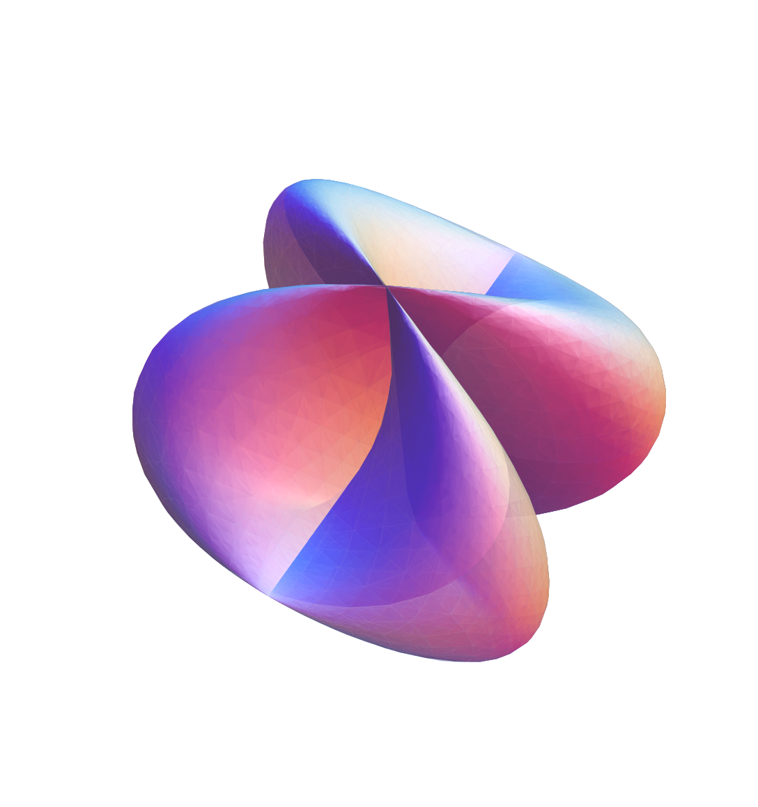
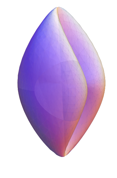
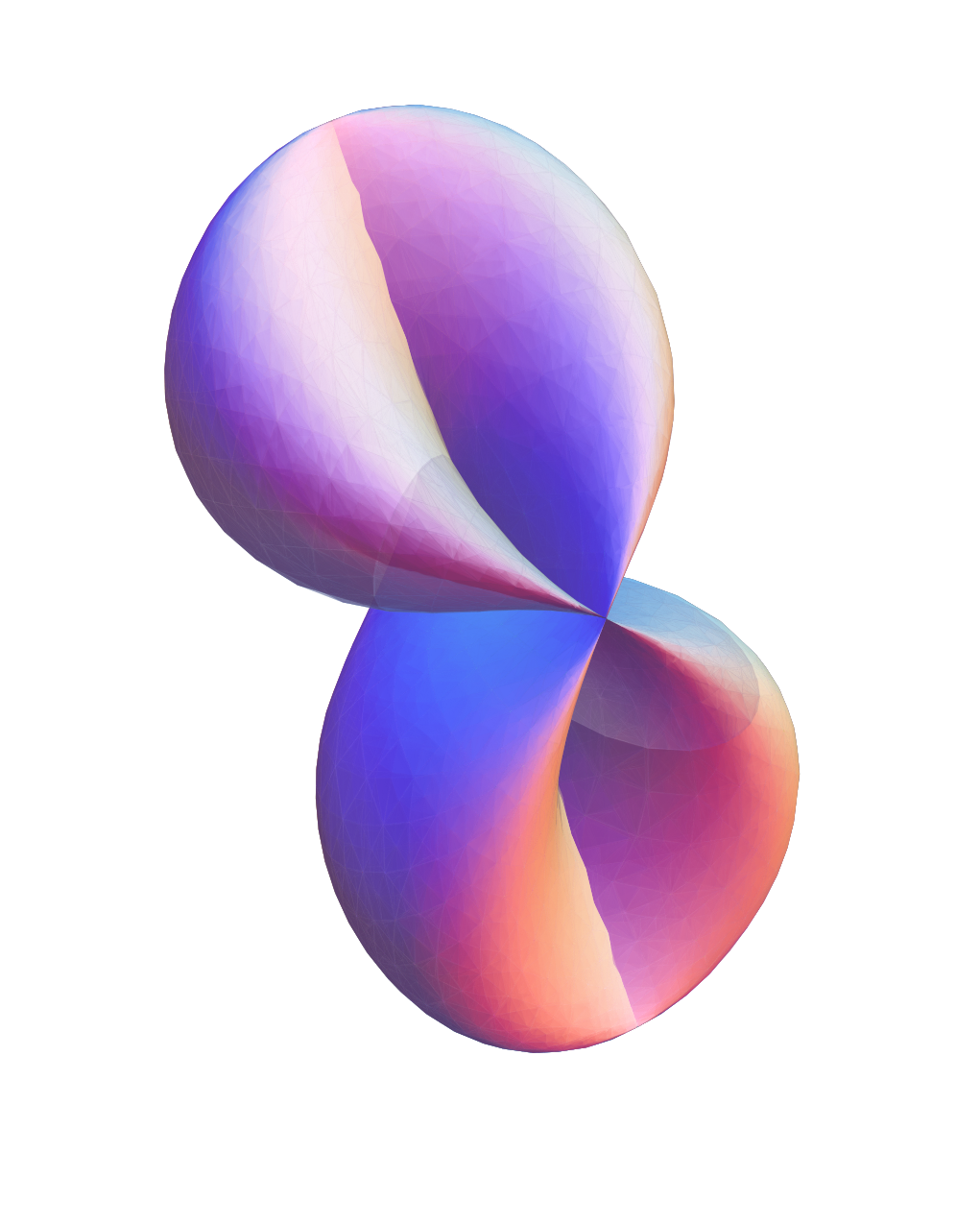
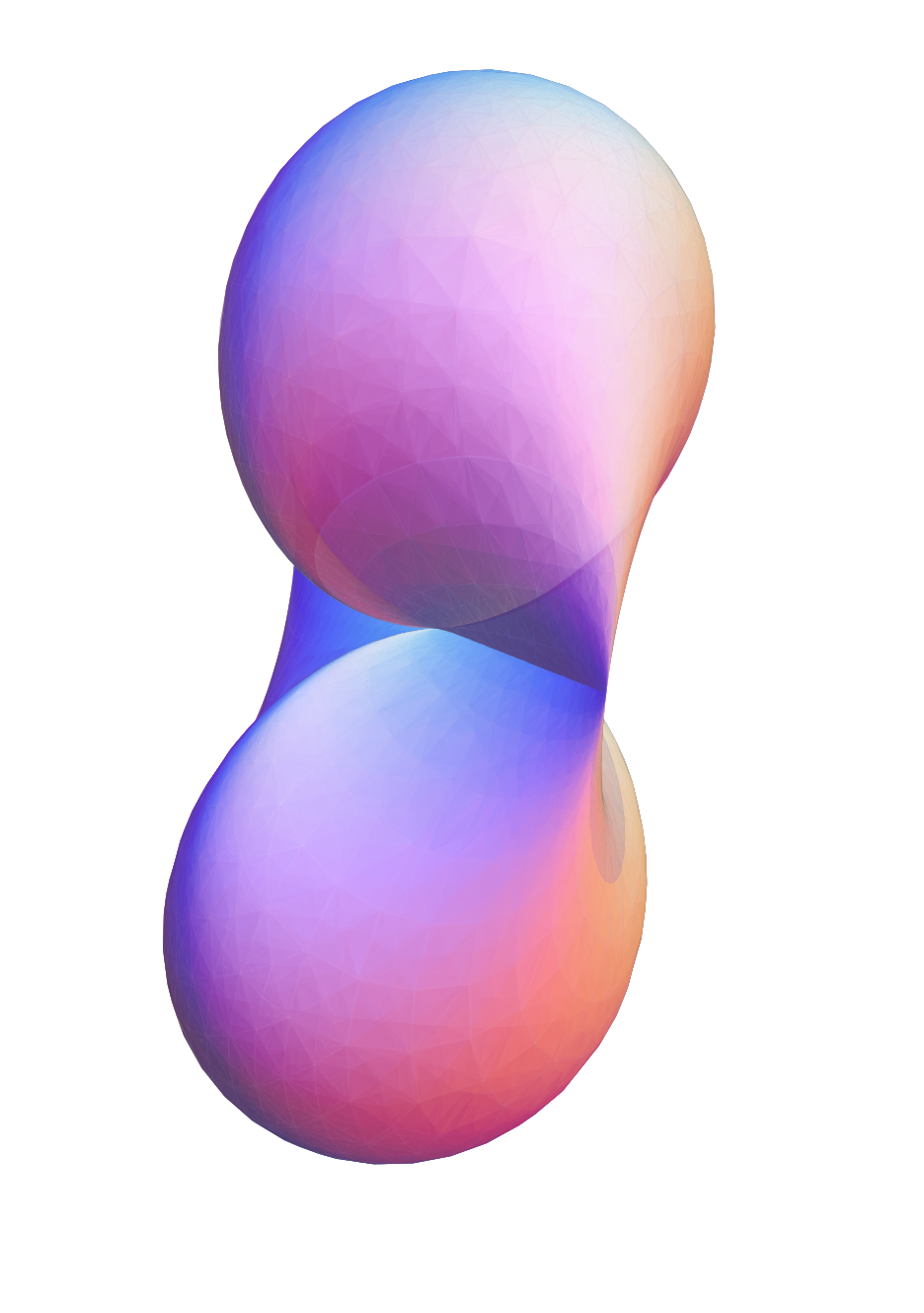
Figure 2. Projections of the Lagrangian torus with $|H|^{2}=9$ to the coordinate 3-spaces of $\mathbb{C}^{2}\equiv\mathbb{R}^{4}$.

3.5. Lagrangian self-similar solitons

An immersion $\phi:M\rightarrow\mathbb{R}^{4}$ is called a self-similar solution for mean curvature flow if

(3.11) $$H=\pm\phi^{\perp}$$

where $\phi^{\perp}$ denotes the normal projection of the position vector $\phi$. If $H=-\phi^{\perp}$ it is called a self-shrinker, and if $H=\phi^{\perp}$ it is called a self-expander. Examples of Lagrangian self-shrinkers and self-expanders can be found in [5].

In the next result we show that the cylinder $\mathbb{S}^{1}\times\mathbb{R}$ is the only (non totally geodesic) self-shrinker for the mean curvature flow in our construction.

Corollary 3.5.

The Lagrangian immersion $\Phi=\alpha\ast\omega$, given in Theorem 2.1, is a (non totally geodesic) self-similar solution for mean curvature flow if and only if $\alpha$ and $\omega$ are both circles of radius one centered at the origin, so that $\Phi=\alpha\ast\omega$ describes the right circular cylinder $\mathbb{R}\times\mathbb{S}^{1}$.

Proof.

We first calculate $\Phi^{\perp}$ as follows:

$$\Phi^{\perp}= \frac{1}{|\alpha|^{2}+|\omega|^{2}}\left(\frac{\mathop{\rm Im}\nolimits\left(\Phi,\Phi_{t}\right)}{|\alpha^{\prime}|^{2}}\,J\Phi_{t}+\frac{\mathop{\rm Im}\nolimits\left(\Phi,\Phi_{s}\right)}{|\dot{\omega}|^{2}}\,J\Phi_{s}\right)$$

$$= \frac{1}{|\alpha^{\prime}|^{2}(|\alpha|^{2}+|\omega|^{2})}\Biggl{(}\frac{|\alpha|^{2}+|\omega|^{2}}{2}\langle\alpha,J\alpha^{\prime}\rangle$$

$$+\left(\int\langle\alpha^{\prime},J\alpha\rangle-\int\langle\dot{\omega},J\omega\rangle\right)\langle\alpha,\alpha^{\prime}\rangle\Biggr{)}J\Phi_{t}$$

$$+\frac{1}{|\dot{\omega}|^{2}(|\alpha|^{2}+|\omega|^{2})}\Biggl{(}\frac{|\alpha|^{2}+|\omega|^{2}}{2}\langle\omega,J\dot{\omega}\rangle$$

$$+\left(\int\langle\dot{\omega},J\omega\rangle-\int\langle\alpha^{\prime},J\alpha\rangle\right)\langle\omega,\dot{\omega}\rangle\Biggr{)}J\Phi_{s}.$$

Taking into account (2.5), we have that $H=\epsilon\,\Phi^{\perp}$, $\epsilon=\pm 1$, if and only if the curvatures of the curves $\alpha$ and $\omega$ satisfy

$$\kappa_{\alpha}= \epsilon\left(\frac{|\alpha|^{2}+|\omega|^{2}}{2}\langle\alpha,J\alpha^{\prime}\rangle+\left(\int\langle\alpha^{\prime},J\alpha\rangle-\int\langle\dot{\omega},J\omega\rangle\right)\langle\alpha,\alpha^{\prime}\rangle\right),$$

$$\kappa_{\omega}= \epsilon\left(\frac{|\alpha|^{2}+|\omega|^{2}}{2}\langle\omega,J\dot{\omega}\rangle+\left(\int\langle\dot{\omega},J\omega\rangle-\int\langle\alpha^{\prime},J\alpha\rangle\right)\langle\omega,\dot{\omega}\rangle\right).$$

Now we derivate the above equations with respect to $s$ and $t$ respectively and we obtain the following necessary condition

(3.12) $$\langle\omega,\dot{\omega}\rangle\langle\alpha,J\alpha^{\prime}\rangle=\langle\dot{\omega},J\omega\rangle\langle\alpha,\alpha^{\prime}\rangle.$$

Using (3.12) together with the conditions on $\kappa_{\alpha}$ and $\kappa_{\omega}$, we get that necessarily $\epsilon=-1$ and so $\Phi$ is a self-shrinker and the only possibility is that the curves $\alpha$ and $\omega$ are both circles centered at the origin. Corollary 3.2 finishes the proof. ∎

3.6. Lagrangian translating solitons

An immersion $\phi:M\rightarrow\mathbb{R}^{4}$ is called a translating soliton for mean curvature flow if

(3.13) $$H={\bf e}^{\perp}$$

for some nonzero constant vector ${\bf e}\in\mathbb{R}^{4}$, where ${\bf e}^{\perp}$ denotes the normal projection of the vector $\bf e$, which can be fixed up to congruences. Examples of Lagrangian translating solitons can be found in [6].

Corollary 3.6.

The Lagrangian immersion $\Phi=\alpha\ast\omega$, given in Theorem 2.1, is a translating soliton with translating vector $\mathbf{e}=\left(\rho\,e^{i\theta},0\right)\in\mathbb{C}^{2}$ if and only if the planar curves $\alpha$ and $\omega$ satisfy that

(3.14) $$|\alpha^{\prime}|\kappa_{\alpha}=\rho\,\mathop{\rm Im}\nolimits\left(e^{-i\,\theta}\alpha^{\prime}\overline{\alpha}\right),\qquad|\dot{\omega}|\kappa_{\omega}=-\rho\,\mathop{\rm Im}\nolimits\left(e^{-i\,\theta}\dot{\omega}\overline{\omega}\right).$$

Remark 3.2.

In Corollary 3.6 we recover, up to dilations and isometries, the Lagrangian translating solitons described in Proposition 3.3 of [6]. The corresponding curves $\alpha$ and $\omega$ are special non trivial solution of the curve shortening problem including spirals and self-shrinking and self-expanding planar curves (see [6] and references therein).

Proof.

We first compute $\left(\rho\,e^{i\theta},0\right)^{\perp}$ for $\Phi=\alpha\ast\omega$:

$$\left(\rho\,e^{i\theta},0\right)^{\perp} =\frac{\rho}{|\alpha|^{2}+|\omega|^{2}}\left(\frac{\mathop{\rm Im}\nolimits\left(\left(e^{i\theta},0\right),\Phi_{t}\right)}{|\alpha^{\prime}|^{2}}\,J\Phi_{t}+\frac{\mathop{\rm Im}\nolimits\left(\left(e^{i\theta},0\right),\Phi_{s}\right)}{|\dot{\omega}|^{2}}\,J\Phi_{s}\right)$$

$$=\frac{\rho}{|\alpha|^{2}+|\omega|^{2}}\left(\frac{\mathop{\rm Im}\nolimits\left(e^{-i\theta}\alpha^{\prime}\overline{\alpha}\right)}{|\alpha^{\prime}|^{2}}J\Phi_{t}-\frac{\mathop{\rm Im}\nolimits\left(e^{-i\theta}\dot{\omega}\overline{\omega}\right)}{|\dot{\omega}|^{2}}J\Phi_{s}\right).$$

Then, taking into account (2.5), we finish the proof. ∎

3.7. Willmore Lagrangians

Consider the Willmore functional

$$\mathcal{W}=\int_{\Sigma}|H|^{2}d\mu$$

for a closed surface $\Sigma$ immersed in Euclidean space. The critical points of $\mathcal{W}$ are known as Willmore surfaces. Examples of Lagrangian Willmore surfaces can be found in [9].

We take $\alpha$ and $\omega$ closed unit speed planar curves. Using Theorem 2.1, the Willmore functional of the Lagrangian conformal immersion $\Phi=\alpha\ast\omega$ is given by

(3.15) $$\mathcal{W}_{\Phi}=\int_{I_{1}\times I_{2}}\left(\kappa_{\alpha}^{2}+\kappa_{\omega}^{2}\right)dtds=L(\omega)\int_{I_{1}}\kappa_{\alpha}^{2}dt+L(\alpha)\int_{I_{2}}\kappa_{\omega}^{2}ds,$$

where $L(\alpha)$ and $L(\omega)$ denote the lengths of $\alpha$ and $\omega$, respectively.

Corollary 3.7.

The Lagrangian immersion $\Phi=\alpha\ast\omega$, given in Theorem 2.1, is a critical point of the Willmore functional $\mathcal{W}_{\Phi}$ (with fixed lengths $L(\alpha)$ and $L(\omega)$) if and only if the curves $\alpha$ and $\omega$ are free elastic curves parametrized by the arc length.

Proof.

From (3.15), the critical points of the Willmore functional $\mathcal{W}_{\Phi}$ (with fixed $L_{1}=L(\alpha)$ and $L_{2}=L(\omega)$) are given by Lagrangian conformal immersions constructed with unit speed planar curves that are critical points of the functionals $\int_{0}^{L_{1}}\kappa_{\alpha}^{2}dt$ and $\int_{0}^{L_{2}}\kappa_{\omega}^{2}ds$, respectively. Since these are precisely free elastic curves according to [14] we finish the proof. ∎

3.8. Lagrangian tori

We now ask about the possibility of obtaining compact Lagrangians from our construction of Theorem 2.1. The following result gives a sufficient condition on the generatrix closed curves to produce Lagrangian tori.

Proposition 3.1.

Let $\alpha=\alpha(t)\subset\mathbb{C}\setminus\{0\}$, $t\in\mathbb{R}$, and $\omega=\omega(s)\subset\mathbb{C}\setminus\{0\}$, $s\in\mathbb{R}$, be regular periodic planar curves, with periods $T$ and $S$ respectively, such that

(3.16) $$\int_{0}^{T}\langle\alpha^{\prime},J\alpha\rangle=0=\int_{0}^{S}\langle\dot{\omega},J\omega\rangle.$$

Then the Lagrangian immersion $\Phi=\alpha\ast\omega$, given in Theorem 2.1, is doubly periodic; concretely, $\Phi(t+T,s)=\Phi(t,s)=\Phi(t,s+S)$, $\forall(t,s)\in\mathbb{R}^{2}$.

Proof.

Under the hypothesis of this proposition, using Remark 2.1, it is clear that $\Phi(t+T,s)=\Phi(t,s)=\Phi(t,s+S)$ if and only if

$$\int_{0}^{t+T}\langle\alpha^{\prime},J\alpha\rangle=\int_{0}^{t}\langle\alpha^{\prime},J\alpha\rangle,\quad\int_{0}^{s+S}\langle\dot{\omega},J\omega\rangle=\int_{0}^{s}\langle\dot{\omega},J\omega\rangle.$$

But using again that $\alpha$ is $T$-periodic and $\omega$ is $S$-periodic, the above conditions are reduced to (3.16). ∎

For example, we can consider a Gerono’s lemniscata (see Figure 3) given by

$$\alpha(t)=\left(1+2\cos t,2\cos t\sin t\right)$$

and a Lissajous curve (see Figure 4) given by

$$\omega(s)=\left(\sin s,\sin(2s)\right).$$

Then it is easy to check that $\Phi=\alpha\ast\omega$ can be written as

$$\Phi(t,s)= \biggl{(}\frac{1}{4}\bigl{(}8\sin^{4}t-2\cos^{2}s-\cos(4s)-8\cos t\bigr{)}$$

$$+\frac{i}{6}\,\bigl{(}9\cos s-\cos(3s)-2\left(9\sin t+3\sin(2t)+\sin(3t)\right)\bigr{)},$$

$$\left(1+\left(2-4\cos s\sin t\right)\cos t\right)\sin s+i\bigl{(}\left(1+2\cos t\right)\sin(2s)+\sin s\sin(2t)\bigr{)}\biggr{)}.$$

In Figure 5 we illustrate the projections of $\Phi=\alpha\ast\omega$ to the coordinate 3-spaces of $\mathbb{R}^{4}$.

Figure 3. Gerono’s lemniscata.

Figure 4. Lissajous curve.

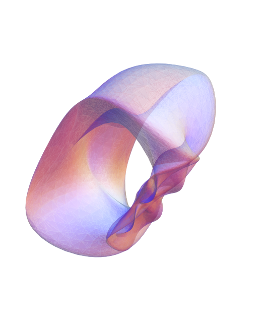
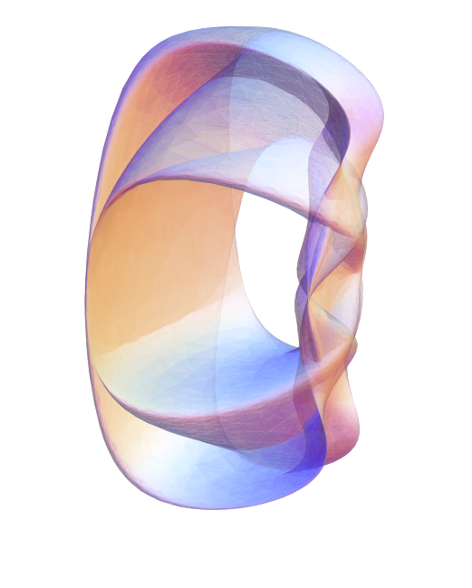
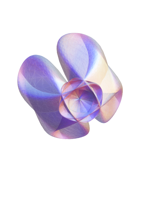
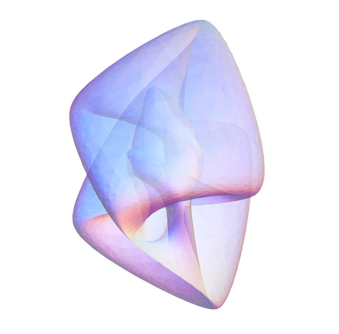
Figure 5. Projections of the torus to the coordinate 3-spaces of $\mathbb{C}^{2}\equiv\mathbb{R}^{4}$.

References

• [1] H. Anciaux. Construction of many Hamiltonian stationary Lagrangian surfaces in Euclidean four-space. Calc. Var. 17 (2003), 105–120.
• [2] H. Anciaux and I. Castro. Constructions of Hamiltonian-minimal Lagrangian submanifolds in complex Euclidean space. Results Math. 60 (2011), 325 -349
• [3] P.F. Byrd and M.D. Friedman. Handbook of Elliptic Integrals for Engineers and Scientists. Springer-Verlag, New-York (1971).
• [4] I. Castro and B.-Y. Chen. Lagrangian surfaces in complex Euclidean plane via spherical and hyperbolic curves. Tohoku Math. J. 58 (2006), 565–579.
• [5] I. Castro and A.M. Lerma. Hamiltonian stationary self-similar solutions for Lagrangian mean curvature flow in complex Euclidean plane. Proc. Amer. Math. Soc. 138 (2010), 1821–1832.
• [6] I. Castro and A.M. Lerma. Translating solitons for Lagrangian mean curvature flow in complex Euclidean plane . Internat. J. Math.  23 (2012), 1250101 (16 pages).
• [7] I. Castro and C. R. Montealegre. A family of surfaces with constant curvature in Euclidean four-space. Soochow J. Math. 30 (2004), no. 3, 293–301.
• [8] I. Castro and F. Urbano. Examples of unstable Hamiltonian-minimal Lagrangian tori in $\mathbb{C}^{2}$. Compositio Math. 111 (1998), 1–14.
• [9] I. Castro and F. Urbano. Willmore surfaces of $\mathbb{R}^{4}$ and the Whitney sphere. Ann. Global Anal. Geom. 19 (2001), 153–175.
• [10] I. Castro and F. Urbano. A characterization of the Lagrangian pseudosphere. Proc. Amer. Math. Soc. 132 (2004), 1797–1804.
• [11] R. Harvey and H.B. Lawson. Calibrated geometries. Acta Math. 148 (1982), 47–157.
• [12] F. Helein and P. Romon. Hamiltonian stationary Lagrangian surfaces in $\mathbb{C}^{2}$. Comm. Anal. Geom. 10 (2002), 79–126.
• [13] D.A. Hoffman and R. Osserman. The geometry of the generalized Gauss map. Mem. Amer. Math. Soc.  236, 1980.
• [14] J. Langer and D. A. Singer. The total squared curvature of closed curves. J. Differential Geom. 20 (1984), no. 1, 1–22.
• [15] Y.G. Oh. Volume minimization of Lagrangian submanifolds under Hamiltonian deformations. Math. Z. 212 (1993), 175–192.
• [16] A. Ros and F. Urbano. Lagrangian submanifolds of $\mathbb{C}^{n}$ with conformal Maslov form and the Witney sphere. J. Math. Soc. Japan 508 (1998), no. 1, 203–226.
• [17] R. Schoen and J.G. Wolfson. Minimizing area among Lagrangian surfaces: the mapping problem. J. Differential Geom. 57 (2001), 301–388.
• [18] A. Strominger, S.T. Yau and E. Zaslow. Mirror symmetry is T-duality. Nuclear Phys. B479 (1996) 243–259.