Self-organization versus top-down planning in the evolution of a city

Abstract

Interventions of central, top-down planning are serious limitations to the possibility of modelling the dynamics of cities. An example is the city of Paris (France), which during the 19th century experienced large modifications supervised by a central authority, the ‘Haussmann period’. In this article, we report an empirical analysis of more than 200 years (1789-2010) of the evolution of the street network of Paris. We show that the usual network measures display a smooth behavior and that the most important quantitative signatures of central planning is the spatial reorganization of centrality and the modification of the block shape distribution. Such effects can only be obtained by structural modifications at a large-scale level, with the creation of new roads not constrained by the existing geometry. The evolution of a city thus seems to result from the superimposition of continuous, local growth processes and punctual changes operating at large spatial scales.

Introduction

A city is a highly complex system where a large number of agents interact, leading to a dynamics seemingly difficult to understand. Many studies in history, geography, spatial economics, sociology, or physics discuss various facets of the evolution of the city Mumford ; Batty ; Angel:book ; Fujita:2001 ; Glaeser:2011 ; Makse:1995 ; Bettencourt:2007 ; Marshall:2009 ; Batty:2009 ; Geddes:1949 . From a very general perspective, the large number and the diversity of agents operating simultaneously in a city suggest the intriguing possibility that cities are an emergent phenomenon ruled by self-organization Batty . On the other hand, the existence of central planning interventions might minimize the importance of self-organization in the course of evolution of cities. Central planning –here understood as a top-down process controlled by a central authority – plays an important role in the city, leaving long standing traces, even if the time horizon of planners is limited and much smaller than the age of the city. One is thus confronted with the question of the possiblity of modelling a city and its expansion as a self-organized phenomenon. Indeed central planning could be thought of as an external perturbation, as if it were foreign to the self-organized development of a city. The recent digitization and georeferentiation of old maps will enable us to test quantitatively this effect, at least at the level of the structure of the road network. Such a transportation network is a crucial ingredient in cities as it allows individuals to work, transport and exchange goods, etc., and the evolution of this network reflects the evolution of the population and activity densities Southworth ; Xie:2009 . These network aspects were first studied in the 1960s in quantitative geography Haggett:1969 , and in the last decade, complex networks theory has provided significant contributions to the quantitative characterization of urban street patterns Jiang:2004 ; Porta:2006 ; Lammer:2006 ; Crucitti:2006 ; Marshall:2006 ; Cardillo:2006 ; Xie:2007 ; Barthelemy:2008 ; Courtat:2011 ; Barthelemy:2011 ; Strano:2012 .

In this article, we will consider the case of the evolution of the street network of Paris over more than 200 years with a particular focus on the 19th century, period when Paris experienced large transformations under the guidance of Baron Haussmann Jordan . It would be difficult to describe the social, political, and urbanistic importance and impact of Haussmann works in a few lines here and we refer the interested reader to the existing abundant literature on the subject (see Samuels:2012 , and Jordan and references therein). Essentially, until the middle of the 19th century, central Paris has a medieval structure composed of many small and crowded streets, creating congestion and, according to some contemporaries, probably health problems. In 1852, Napoleon III commissioned Haussmann to modernize Paris by building safer streets, large avenues connected to the new train stations, central or symbolic squares (such as the famous place de l’Etoile, place de la Nation and place du Panthéon), improving the traffic flow and, last but not least, the circulation of army troops. Haussmann also built modern housing with uniform building heights, new water supply and sewer systems, new bridges, etc (see Fig. 1 where we show how dramatic the impact of Haussmann transformations are).

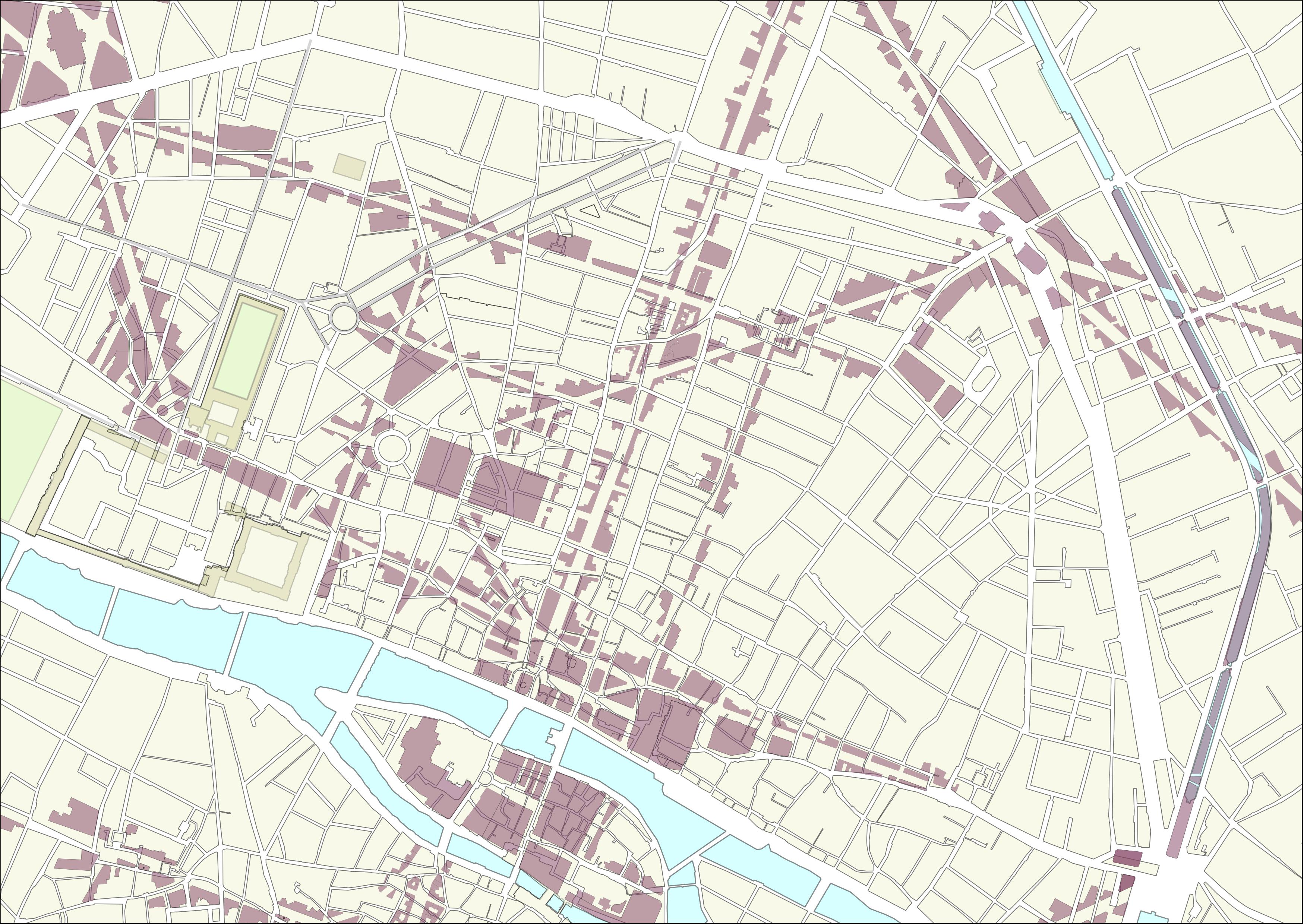
Figure 1: Illustration on a small area of the impact of Haussmann’s transformations. On the yellow background, we show the parcel distribution before Haussmann (extracted from the Vasserot cadastre, 1808-1836), and in brown we show the new buildings delineating the new streets as designed by Haussmann and as they appeared in 1888. We can see on this example that the Haussmann plan implied a large number of destruction and rebuilding: approximately $28,000$ houses were destroyed and $100,000$ were built Samuels:2012 (figure created from our data).

The case of Paris under Haussmann provides an interesting example where changes due to central planning are very important and where a naive modelling is bound to fail. We analyze here in detail the effect of these planned transformations on the street network. By introducing physical quantitative measures associated with this network, we are able to compare the effect of the Hausmann transformation of the city with its ‘natural’ evolution over other periods.

By digitizing historical maps (for details on the sources used to construct the maps, see the Methods section) into a Geographical Information System (GIS) environment, we reconstruct the detailed road system (including minor streets) at six different moments in time, $t=1,2,\ldots,6$, respectively corresponding to years: $1789,1826,1836,1888,1999,2010$. For each time, we constructed the associated primal graph $G_{t}$ (see the Methods section and  Barthelemy:2011 ; Strano:2012 ), i.e. the graph where the nodes represent street junctions and the links correspond to road segments. In particular, it is important to note that we have thus snapshots of the street network before Haussmann works (1789-1836) and after (1888-2010). This allows us to study quantitatively the effect of such central planning.

In Fig. 2(a), we display the map of Paris as it was in 1789 on top of the current map (2010).

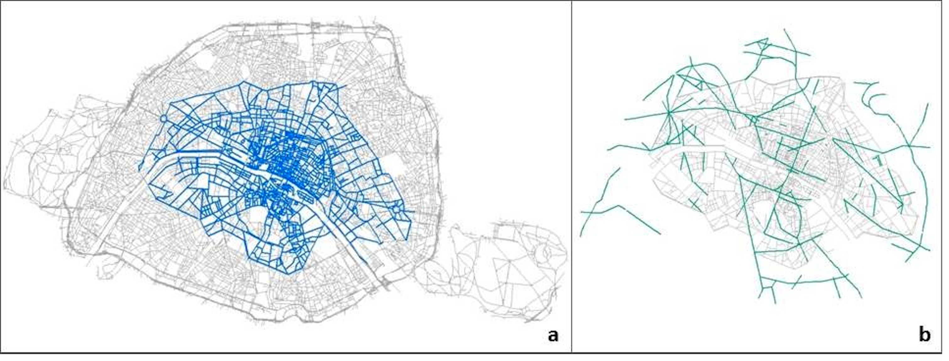
Figure 2: (a) Map of Paris in 1789 superimposed on the map of current 2010 Paris. In the whole study, we focus on the Haussmann modifications and limited ourselves to the 1789 portion of the street network. (b) Map of Haussmann modifications. The grey lines represent the road network in 1836, the green lines represent the Haussmann modifications which are basically all contained in the 1789 area (figure created from our data).

In order to use a single basis for comparison, we limited our study over time to the portion corresponding to 1789. We note here that the evolution of the outskirts and small villages in the surroundings has certainly an impact on the evolution of Paris and even if we focus here (mainly because of data availability reasons) on the structural modifications of the inner structure of Paris, a study at a larger scale will certainly be needed for capturing the whole picture of the evolution of this city. We then have 6 maps for different times and for the same area (of order $34km^{2}$). We also represent on Fig. 2(b), the new streets created during the Haussmann period which covers roughly the second half of the 19th century. Even if we observe some evolution outside of this portion, most of the Haussmann works are comprised within this portion.

Results

Simple measures.

In the following we will study the structure of the graph $G_{t}$ at different times $t$ (see the Methods section for precise definitions), having in mind that our goal is to identify the most important quantitative signatures of central planning during the evolution of this road network.

First basic measures include the evolution of the number of nodes $N$, edges $E$, and total length $L_{tot}$ of the networks (restricted to the area corresponding to 1789). In Fig. 3 we show the results for these indicators which display a clear acceleration during the Haussmann period (1836-1888).

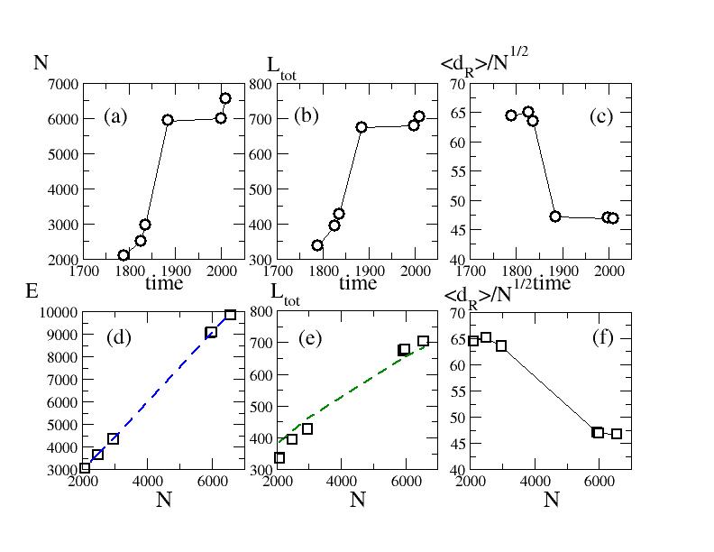
Figure 3: Top panels: Number of (a) nodes, (b) total length (kms), and (c) rescaled average route distance versus time. Bottom panels: Number of (d) edges, (e) total length (kms), and (f) the rescaled average route distance versus the number of nodes $N$. In (d) the dashed (blue) line is a linear fit with slope $1.55$ ($r^{2}=0.99$) consistent with constant average degree of order $\langle k\rangle\approx 3$, and in (e) the dashed (green) line a square root fit of the form $a\sqrt{N}$ with $a=8.44$kms ($r^{2}=0.99$). Based on a perturbed lattice picture this gives an area equal to $A\simeq 29.7$km² consistent with the actual value ($A=33.6$km²). In (f), we show the rescaled average shortest route versus $N$ which decreases showing that the denser the network and the easier it is to navigate from one node to the other (if delays at junctions are neglected).

The number of nodes increased from about 3000 in 1836 to about 6000 in 1888 and the total length increase from about 400 kms to almost 700kms, all this in about 50 years. It is interesting to note that this node increase corresponds essentially to an important increase in the population. In particular, we note (see the Supplementary Information for more details) that the number of nodes $N$ is proportional to the population $P$ and that the corresponding increase rate is of order $dN/dP\approx 0.0021$, similar to what was measured in a previous study about a completely different area Strano:2012 . The rapid increase of nodes during the Haussmann period is thus largely due to demographic pressure. Now, if we want to exclude exogeneous effects and focus on the structure of networks, we can plot the various indicators such as the number of edges and the total length versus the number of nodes taken as a time clock. The results shown Fig. 3(d-f) display a smoother behavior. In particular, $E$ is a linear function of $N$, demonstrating that the average degree is essentially constant $\langle k\rangle\approx 3.0$ since 1789. The total length versus $N$ also displays a smooth behavior consistent with a perturbed lattice Barthelemy:2011 . Indeed, if the segment length $\ell_{1}$ is roughly constant and equal to $\ell_{1}=1/\sqrt{\rho}$ where $\rho=N/A$ is the density of nodes ($A$ is the area considered here), we then obtain for the total length

$$L_{tot}=\frac{\langle k\rangle}{2}\sqrt{AN}$$ (1)

A fit of the type $a\sqrt{N}$ is shown in Fig. 3(d) and the value of $a$ measured gives an estimate of the area $A\simeq 29.7km^{2}$, in agreement with the actual value $A=33.6km^{2}$ (for the 1789 portion). This agreement demonstrates that all the networks at different times are not far from a perturbed lattice.

We also plot the average route distance $d_{R}$ defined as the average over all pairs of nodes of the shortest route between them (see Methods for more details). For a two dimensional spatial network, we expect this quantity to scale as $d_{R}\sim\sqrt{N}$ and thus increases with $N$. The ratio $d_{R}/\sqrt{N}$ is thus better suited to measure the efficiency of the network and we observe (Fig. 3(c,f)) that it decreases with time and $N$. This result simply demonstrate that if we neglect delays at junctions, it becomes easier to navigate in the network as it gets denser.

Typology of new links

We can have three different types of new links depending on the number of new nodes they connect. We denote by $E_{i}$ ($i=1,2,3$) the number of new links appearing at time $t+1$ connecting $i$ new nodes. For example $E_{0}$ counts the new links appearing at time $t+1$ connecting two nodes existing at time $t$. In order to categorize more precisely these new links, we use the betweenness centrality impact $\delta$ defined in Strano:2012 and which measures how a new link (absent at time $t$ and present at time $t+1$) affects the average betweenness centrality (see Methods section for definitions of the betweenness centrality impact $\delta$). In Strano:2012 , the distribution of this quantity displays two peaks which corresponds to two types of links belonging to two distinct processes: densification and exploration Strano:2012 . We first observe (see Figure 2 of SI) that in the first period, the majority of new links are of the $E_{2}$ type and correspond to construction of new streets with new nodes. We see that the Haussmann transition period (1836-1888) is not particularly different from the other previous periods. In the modern period (after 1999), $E_{0}$ becomes dominant and consistent with the idea of a mature street network where densification dominates the evolution of the urban tissue. Obviously, this is also an effect of limiting ourselves to the 1789 portion: in a wider area, many new roads were created and both densification and exploration coexist. We note here that the structure of the street network of central Paris remained remarkably stable from 1888 until now (and in this period also, densification was the main process in this area).

We then plot the distribution of this quantity $\delta$ for the different transition periods and the result is shown in Fig. 4.

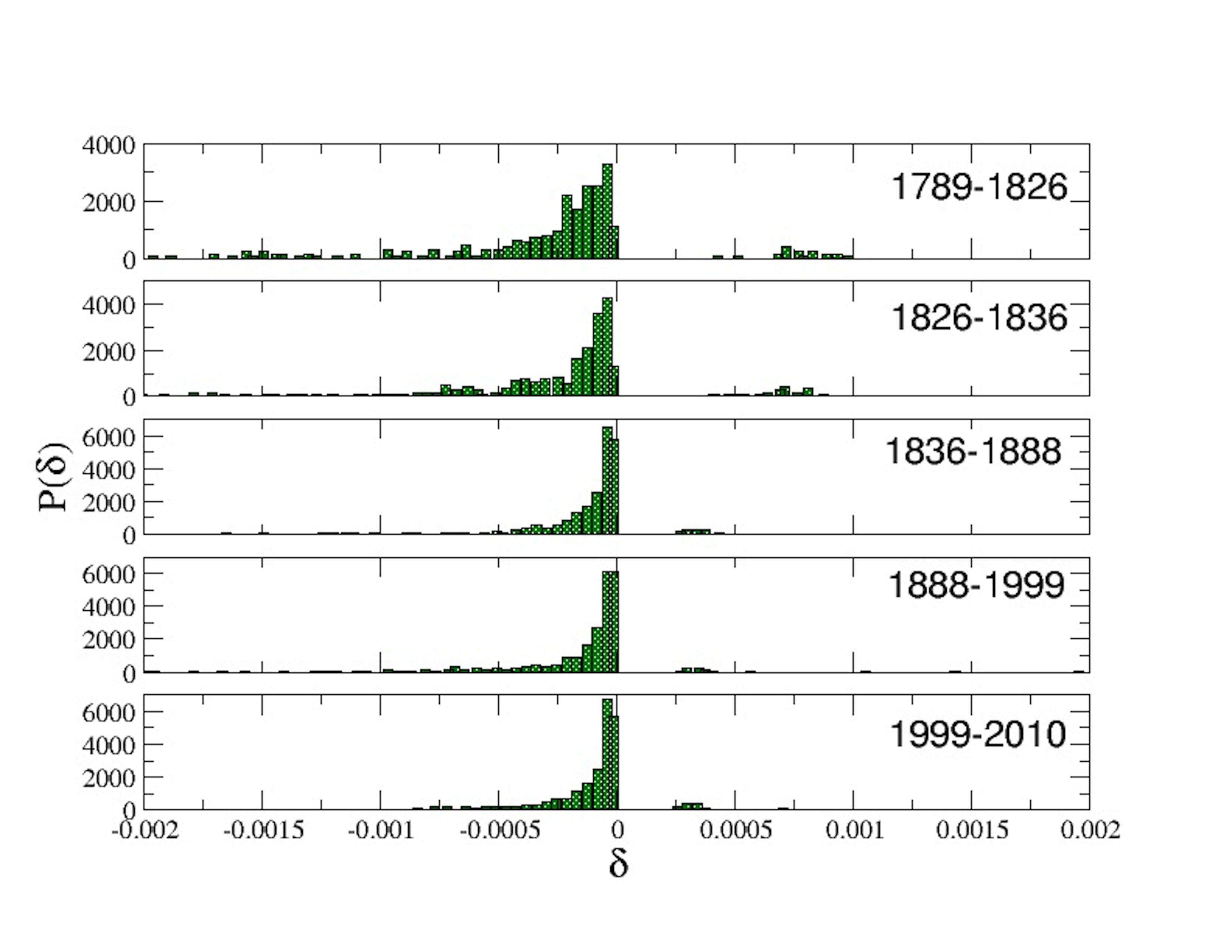
Figure 4: Betweenness centrality impact distribution for the periods $1789\rightarrow 1826$, $1826\rightarrow 1836$, $1836\rightarrow 1888$, $1888\rightarrow 1999$, $1999\rightarrow 2010$. This figure shows that densification is the main process for this portion of Paris and that from this point of view, the Haussmann period seems to be rather smooth and comparable to other periods.

These figures show that for all periods most new links belong to the densification process with a small peak of exploration in the period 1836-1888. In well-developed, mature systems, it is expected that densification is the dominant growth mechanism. Here also, we see that the Haussmann period is not significantly different from previous periods.

Evolution of the spatial distribution of centrality

The betweenness centrality (BC) $g_{v}(i)$ of a node $i$ is defined in the Methods section and essentially measures the fraction of times a given node is used in the shortest paths connecting any pair of nodes in the network, and is thus a measure of the contribution of a link in the organisation of flows in the network Freeman:1977 . In our case where we consider a limited portion of a spatial network, two important effects need to be taken into consideration. First, as we consider a portion, only paths within this portion are taken into account in the calculation of the BC and this usually does not reflect the reality of the actual origin-destination matrix. In particular, flows with the exterior of the portion and surrounding villages are not taken into account. As a result, the BC will be able to detect important routes and nodes in the internal structure of the network but will miss large-scale communication roads such as a north-south or east-west road connecting the portion with the surroundings of Paris. In Strano:2012 , the scale of the network was large enough so that the BC could recover important central roads such as Roman streets. The BC in the present case has then to be used as a structural probe of the network, enabling us to track the important modifications. The second point concerns the spatial distribution of the BC which will be important in the following. For a lattice the most central nodes (see the discussion in Barthelemy:2011 for example) are close to the barycenter of the nodes: spatial centrality and betweenness centrality are then usually strongly correlated. In Lammer:2006 and Crucitti:2006 it is shown that the most central points display interesting spatial structures which still need to be understood, but which represent an important signature of the networks’ topology.

We first consider the time evolution of the node betweenness centrality (with similar results for the edge BC). In the SI (see figure 3 of SI), we show the distribution of the node BC at different times. Apart from the fact that the average BC varies, we see that the tail of the distribution remains constant in time, showing that the statistics of very central nodes is not modified. From this point of view, the evolution of the road network follows a smooth behavior, even in the Haussmann period.

So far, most of the measures indicate that the evolution of the street network follows simple densification and exploration rules and is very similar to other areas studied Strano:2012 . At this point, it appears that Haussmann works didn’t change radically the structure of the city. However, we can suspect that Haussmann’s impact is very important on congestion and traffic and should therefore be seen on the spatial distribution of centrality. In the figure 5, we show the maps of Paris at different times and we indicate the most central nodes (such that their centrality $g_{v}(i)$ is larger than $\max{g_{v}}/\alpha$ with $\alpha=10$ see the SI, for a discussion on the effect of the value of $\alpha$).

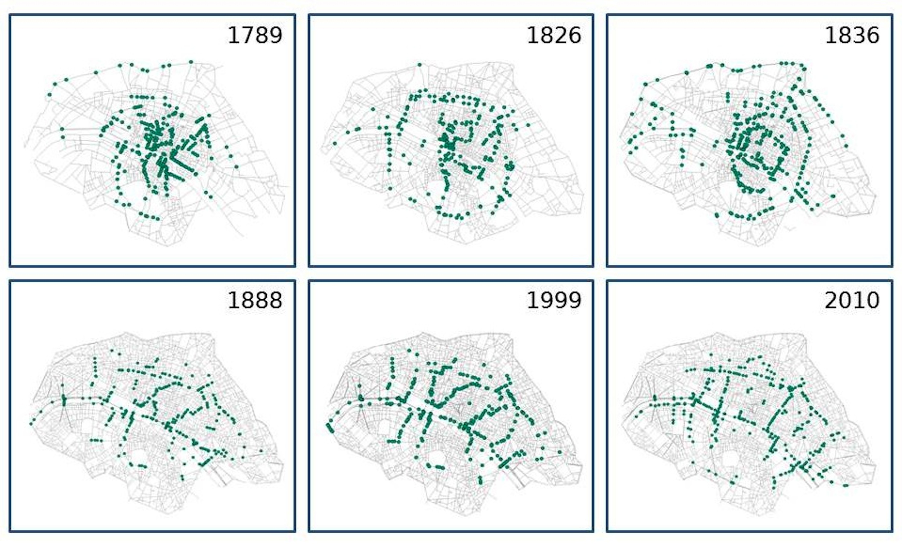
Figure 5: Spatial distribution of the most central nodes (with centrality $g_{v}$ such that $g_{v}>\max{g_{v}}/10$). We observe for the different periods important reorganizations of the spatial distribution of centrality, corresponding to different specific interventions. In particular, we observe a very important redistribution of centrality during the Haussmann period with the appearance of a reticulated structure on the 1888 map.

We can clearly see here that the spatial distribution of the BC is not stable, displays large variations, and is not uniformly distributed over the Paris area (we represented here the node centrality, and similar results are obtained for the edge centrality, see the SI for plots for the edge centrality and more details). In particular, we see that between 1836 and 1888, the Haussmann works had a dramatical impact on the spatial structure of the centrality, especially near the heart of Paris. Central roads usually persist in time Mouton:1989 ; Strano:2012 , but in our case, the Haussmann reorganization was acting precisely at this level by redistributing the shortest paths which had certainly an impact on congestion inside the city. After Haussmann we observe a large stability of the network until nowadays.

It is interesting to note that these maps also provide details about the evolution of the road network of Paris during other periods which seems to reflect what happened in reality and which we can relate to specific local interventions. For example, in the period 1789-1826 between the French Revolution and the Napoleonic empire, the maps shown in Fig. 5 display large variations with redistribution of central nodes which probably reflects the fact that many religious and aristocratic domains and properties were sold and divided in order to create new houses and new roads, improving congestion inside Paris. During the period 1826-1836 which corresponds roughly to the beginning of the the July Monarchy, the maps in Fig. 5 suggests an important reorganization on the east side of Paris. This seems to correspond very well to the creation during that period of a new channel in this area (the channel ‘Saint Martin’) which triggered many transformations in the eastern part of the network.

In order to analyse the spatial redistribution effect more quantitatively, we compute various quantities inside a disk of radius $r$ centered on the barycenter of all nodes (which stays approximately at the same location in time). We first study the number of nodes $N(r)$ (Fig. 6), its variation $\delta N(r)$ between $t$ and $t+1$, and the number of central nodes (such that $g_{v}(i)>\max{g_{v}}/10$).

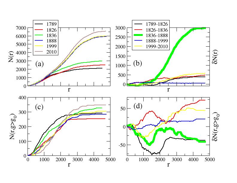
Figure 6: Top panels: (a) number of nodes in a disk of radius $r$ from the barycenter of Paris and (b) its variation versus $r$. As expected the largest variation occurred during the Haussmann period. (c) Number of nodes at distance $r$ and with centrality larger than $g_{0}$ ($g_{0}=\max{g_{v}}/10$) and (d) its variation. The thick green line in the right panels indicate the Haussmann transition 1836-1888. We see here that during the Haussmann period (and also in the 1789-1826 period), there is a large decrease of the number of central nodes in the central region of Paris ($r<2,000$ meters).

We see that the largest variation of the number of nodes (see 6(b)) is indeed in the Haussmann period 1836-1888, especially for distance $r>1,500$ meters. More interesting, is the variation of the most central nodes (Fig. 6d). In particular, we observe that during the pre-Haussmann period, even if in the period 1789-1826 there was an improvement of centrality concentration, there is an accumulation of central nodes both at short distances ($r<2,500$ meters) and at long distances ($r>2,500$ meters) in the following period (1826-1836). As a result, visually clear in Fig. 5, there is a large concentration of centrality in the center of Paris until 1836 at least. The natural consequence of this concentration is that the center of Paris was very probably very congested at that time. In this respect, what happens under the Haussmann supervision is natural as he acts on the spatial organization of centrality. We see indeed that in 1888, the most central nodes form a more reticulated structure excluding concentration of centrality. A structure which remained stable until now. Interestingly, we note that Haussmann’s new roads and avenues represent approximately $6\%$ of the total length only (compared to nowadays network), which is a small fraction, considered that it has a very important impact on the centrality spatial organization.

This reorganization of centrality was undertaken with creation of new roads and avenues destroying parts of the original pattern (see Fig. 1 and Fig. 2(b)) resulting in the modification of the geometrical structure of blocks (defined here as the faces of the planar street network). The effect of Haussmann modifications on the geometrical structure of blocks can be quantitatively measured by the distribution of the shape factor $\phi$ (see Methods) shown in Fig. 7.

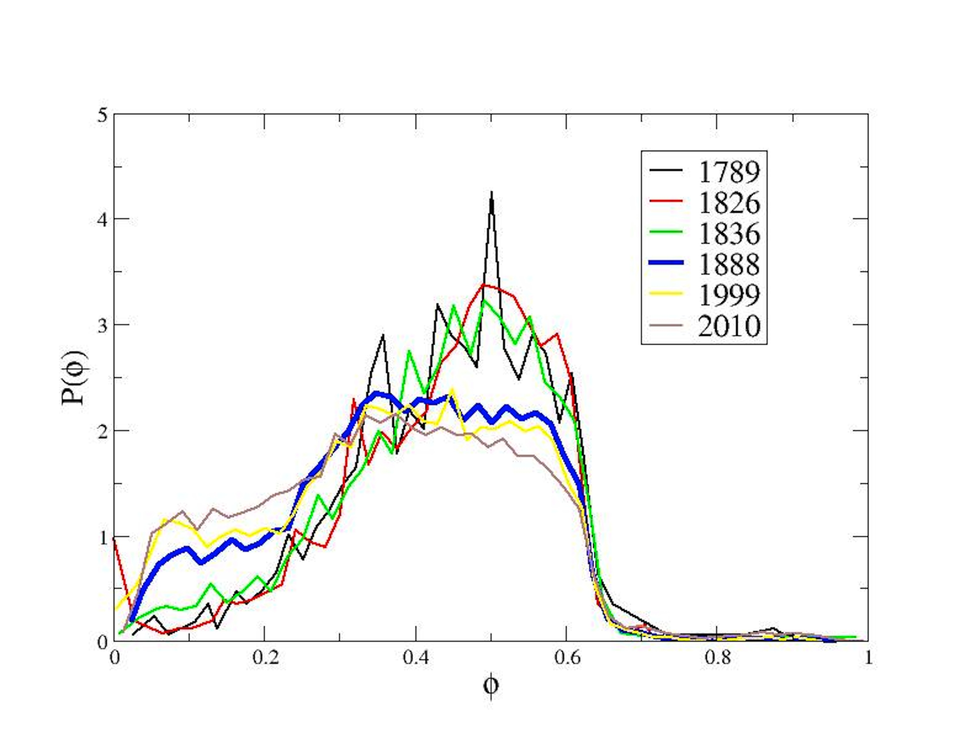
Figure 7: Probability distribution of the $\phi$ shape factor for the blocks at different years. Until 1836, this distribution is stable and we observe a dramatical change during the Haussmann period with a larger abundance of blocks with small value of $\phi$. These small values correspond to elongated rectangle or triangles created by streets crossing the existing geometry at various angles.

We see that before the Haussmann modifications, the distribution of $\phi$ is stable and is essentially centered around $\phi=0.5$ which corresponds to rectangles. From 1888, the distribution is however much flatter showing a larger diversity of shapes. In particular, we see that for small values of $\phi<0.25$ there is an important increase of $P(\phi)$ demonstrating an abundance of elongated shapes (triangles and rectangles mostly) created by Haussmann’s works. These effects can be confirmed by observing the angle distribution of roads shown on Fig. 8 where we represent on a polar plot $r(\theta)=P(\theta)$ with $P(\theta)$ the probability that a road segment makes an angle $\theta$ with the horizontal line.

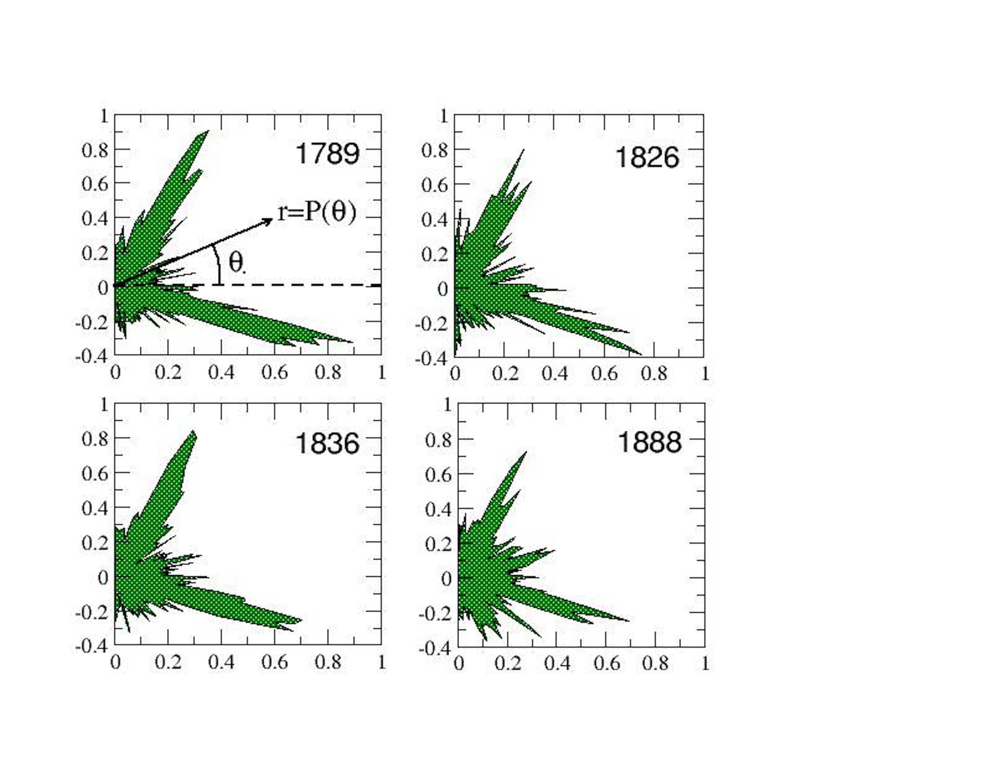
Figure 8: Radial representation of the angle distribution of road segments for 1789, 1826, 1836, 1888. The radial distance $r$ in this plot represents the probability to observe a street with angle $\theta$: $r=P(\theta)$ with $\theta\in[-\pi/2,\pi/2]$ and $P(\theta)$ is the probability to observe an oriented road with angle $\theta$ with the horizontal line (see first panel, top left). Until 1836, the distribution is peaked around two values separated by approximately $90$ degrees and in 1888, we observe an important fraction of diagonals and other lines at intermediate angles.

Before Haussmann’s modifications, the distribution has two clear peaks corresponding to perpendicular streets and in 1888 we indeed observe a more uniform distribution with a large proportion of various angles such as diagonals.

Discussion

In this paper, we have studied the evolution of the street network of the city of Paris. This case is particularly interesting as Paris experienced large modifications in the 19th century (the Haussmann period) allowing us to try to quantity the effect of central planning. Our results for central Paris reveal that most indicators follow a smooth evolution, dominated by a densification process, despite the important perturbation that happened during Haussmann. In our results, the important quantitative signature of central planning is the spatial reorganization of the most central nodes, in contrast with other regions where self-organization dominated and which didn’t experience such a large-scale structure modification. This structural reorganization was obtained by the creation at a large scale of new roads and avenues (and the destruction of older roads) which do not follow the constraints of the existing geometry. These new roads do not follow the densification/exploration process but appear at various angles and intersect with many other existing roads.

While the natural, self-organized evolution of roads seems in general to be local in space, the Haussmann modifications happen during a relatively short time and at a large spatial scale by connecting important nodes which are far away in the network. Following the Haussmann interventions, the natural processes take over on the modified substrate. It is unclear at this stage if Haussmann modifications were optimal and more importantly, if they were at a certain point inevitable and would have happened anyway (due to the high level of congestion for example). More work, with more data on a larger spatial scale are probably needed to study these important questions.

Methods

Temporal Network Data

We denote by $G_{t}\equiv G(V_{t},E_{t})$ the obtained primal graph at time $t$, where $V_{t}$ and $E_{t}$ are respectively the set of nodes and links at time $t$. The number of nodes at time $t$ is then $N(t)=|V_{t}|$ and the number of links is $E(t)=|E_{t}|$. Using common definitions, we thus have $V_{t}=V_{t-1}\cup\Delta V_{t}$ and $E_{t}=E_{t-1}\cup\Delta E_{t}$, where $\Delta V_{t}$ and $\Delta E_{t}$ are respectively the new street junctions and the new streets added in time $]t-1,t]$ to the network existing at time $t-1$.

The networks for 1789, 1826, 1836, 1888 are extracted from the following maps:

• 1789: Map of the city of Paris with its new enclosure. Geometrically based on the ‘meridienne de l’Observatoire’ and surveyed by Edmé Verniquet. Achieved in 1791.

• 1826: Road map of Paris surveyed by Charles Picquet, geographer for the King and the duke of Orléans.

• 1836: Cadastre of Paris, Philibert Vasserot. Map constructed according blocks and classified according to old districts. 24 Atlas, 1810-1836.

• 1888: Atlas of the 20 districts of Paris, surveyed by M. Alphand, and L. Fauve, under the administration of the prefect E. Poubelle, Paris, 1888.

All these maps were digitized at the LaDéHiS under the supervision of Maurizio Gribaudi, in the framework of a research on the social and architectural transformations of parisian neighborhoods between the 18th and 19th centuries. The network (and the block structure of figure 1) extracted from the Vasserot cadastre was initiated by Anne-Laure Bethe for the program Alpage Alpage .

The networks of 1999 and 2010 are coming from the french Geographical National Institute (IGN) on the basis of modern surveys.

Average route distance

For a network, the shortest path between two nodes is defined as the path with the minimum number of links connecting the two nodes. For spatial networks, it makes more sense to weight the links with their length: to each edge $e$ we thus associate a weight given by its euclidean length $d_{e}$. We can then compute the length $\ell$ of a path $P$

$$\ell(P)=\sum_{e\in P}d_{e}$$ (2)

The shortest weighted path is then the one with the minimum total length. The average shortest weighted path is also called the average route distance $d_{R}$. It indicates on average how many kilometers you have to walk from one point to the other in this spatial network. For a two dimensional network, it is expected Barthelemy:2011 that it scales as

$$d_{R}\sim N^{1/2}$$ (3)

for a network of size $N$. In order to compare networks with different numbers of nodes $N$, it is then natural to compare the rescaled average route distance $d_{R}/\sqrt{N}$.

Betweenness centrality, Impact

The nature of the growth process can be quantitatively characterised by looking at the centrality of streets. Among the various centrality indices available for spatial networks we use here the betweenness centrality (BC) Freeman:1977 ; Crucitti:2006 ; Porta:2006 , which is one of the measures of centrality commonly adopted to quantify the importance of a node or a link in a graph. Given the graph $G_{t}\equiv G(V_{t},E_{t})$ at time $t$, the BC of a link $e$ is defined as:

$$g(e)=\sum_{i\in V}\sum_{\stackrel{{\scriptstyle j\in V}}{{j\neq i}}}\frac{\sigma_{ij}(e)}{\sigma_{ij}}$$ (4)

where $\sigma_{ij}$ is the number of shortest paths from node $i$ to node $j$, while $\sigma_{ij}(e)$ is the number of such shortest paths which contain the link $e$. The quantity $g(e)$ essentially measures the number of times a link is used in the shortest paths connecting any pair of nodes in the network, and is thus a measure of the contribution of a link in the organisation of flows in the network. The BC of a node is defined in a similar way

$$g_{v}(i)=\sum_{s,t\in V}\frac{\sigma_{st}(i)}{\sigma_{st}}$$ (5)

where $\sigma_{st}(i)$ denotes here the number of shortest path from node $s$ to $t$ going through the node $i$.

In order to evaluate the impact of a new link on the overall distribution of the betweenness centrality we use the betweenness centrality impact defined in Strano:2012 . In the graph at time $t$, we first compute the average betweenness centrality of all the links of $G_{t}$ as:

$$\overline{g}(G_{t})=\frac{1}{(N(t)-1)(N(t)-2)}\sum_{e\in E_{t}}g(e)$$ (6)

where $g(e)$ is the betweenness centrality of the edge $e$ in the graph $G_{t}$. Then, for each link $e^{*}\in\Delta E_{t}$, i.e. for each newly added link in the time window $]t-1,t]$ we consider the new graph obtained by removing the link $e^{*}$ from $G_{t}$ and we denote this graph as $G_{t}\setminus\{e^{*}\}$. We compute again the average edge betweenness centrality, this time for the graph $G_{t}\setminus\{e^{*}\}$. Finally, the impact $\delta(e^{*})$ of edge $e^{*}$ on the betweenness centrality of the network at time $t$ is defined as

$$\delta(e^{*})=\frac{\left[\overline{g}(G_{t})-\overline{g}(G_{t}\setminus\{e^{*}\})\right]}{\overline{g}(G_{t})}$$ (7)

The BC impact is thus the relative variation of the graph average betweenness due to the removal of the link $e^{*}$.

Form factor

The shape or form factor $\phi$ of blocks is defined as the ratio of the area of the block and the area of the circumscribed circle of diameter $D$ (see Lammer:2006 ; Barthelemy:2011 )

$$\phi=\frac{A}{\pi D^{2}/4}$$ (8)

The more anisotropic the block and the smaller the factor $\phi$.

Supplementary Information

.1 Population and nodes

In figure 9, we show the evolution of the number of nodes and of the population of Paris (for the 12 districts delimited by the ‘fermiers generaux’ for the period 1789-1851 and after for the 20th districts of Paris).

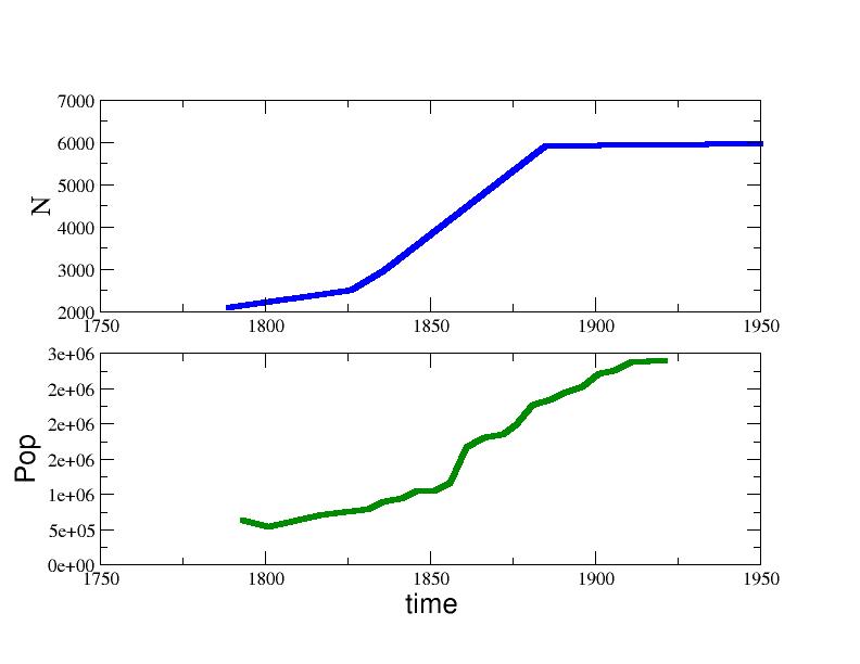
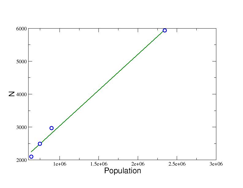
Figure 9: Top panel: Evolution of the number of nodes versus time for Paris. Middle panel: evolution of the Paris population. Bottom panel: Number of nodes versus population. The line is a linear fit ($r^{2}>0.99$).

The area under consideration for the calculation of the population is not exactly the same, and only the order of magnitude can be trusted here. We can compute the number of nodes $N$ versus the population $P$ and we observe a linear dependence with coefficient $dN/dP=0.0021$ (in previous studies, we also found a linear dependence [24], but with a linear coefficient equal to $dN/dP=0.019$). It is thus clear that the number of nodes follows the demographic population and that the large increase observed during the Haussmann period is largely due to the demographic pressure.

.2 Type of new links

In figure 10, we show the evolution of the proportion of the different types of new links. We see in this figure that the evolution is rather smooth and that from this point of view, the Haussmann period is not radically different from previous ones.

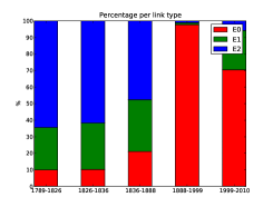
Figure 10: Evolution of the percentage of different types of links. $E_{i}$ corresponds to new links with creation of $i$ new nodes. The denser the network, the smaller $E_{2}$ and in particular, we observe that the Haussmann period is not radically different in this respect from other periods.

.3 Stability of the BC distribution

We consider here the evolution of the vertex BC with time. In figure 11, we see that the average BC decreases slightly and that the overall probability distribution remains constant in time.

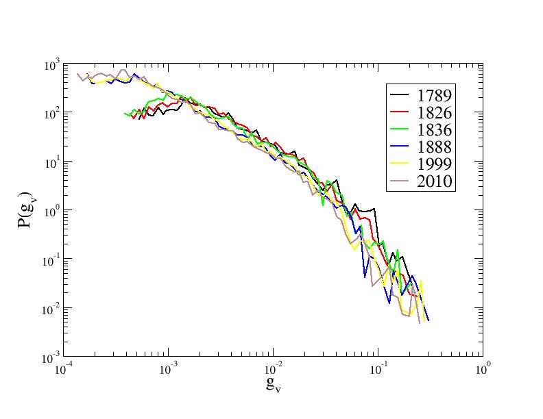
Figure 11: Vertex BC distribution for all links and all periods. Vertex BC probability distribution for the different time snapshots considered in this study. We note that the average BC decreases (indicating a larger navigability in the system) and that the overall shape and tail remain the same across all times.

.4 Most central nodes: stability of spatial patterns

The most central nodes are such as their centrality is $g_{v}>\max{g_{v}}/\alpha$. In the letter we consider $\alpha=10$ and we show in figure 12 the results for $\alpha=5$ and $\alpha=15$. A visual inspection shows that the patterns are rather robust versus $\alpha$ and that $\alpha=10$ corresponds to an intermediate situation displaying interesting patterns.

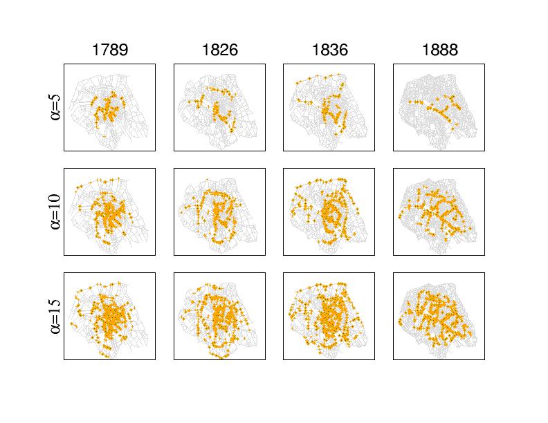
Figure 12: Spatial patterns of most central points defined by $g_{v}>\max{g_{v}}/\alpha$ for different values of $\alpha$. We see that for the 4 time points considered here that the pattern is robust with respect to the value of $\alpha$.

.5 Spatial pattern of the most central edges

Instead of the most central nodes, we can also represent the most central edges such that their centrality is $g_{e}>\max{g_{e}}/\alpha$. If we consider here $\alpha=20$ we obtain for the different dates the results presented in Fig. 13.

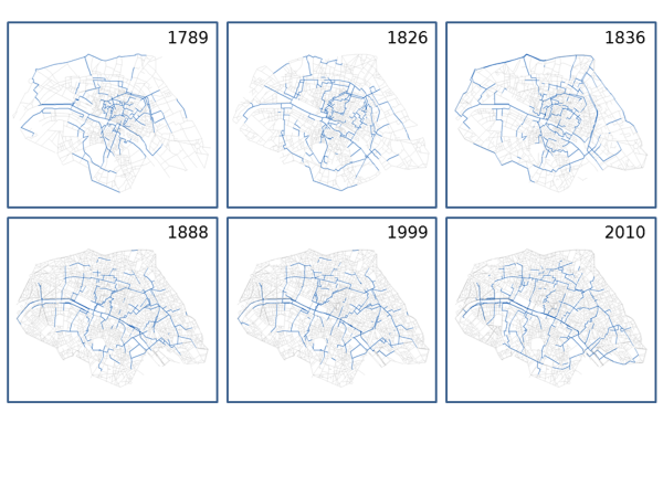
Figure 13: Spatial patterns of most central edges defined by $g_{e}>\max{g_{e}}/\alpha$ for $\alpha=20$.

We can see that the pattern for the edges is naturally consistent with the one obtained with the node centrality.

References

Acknowledgements. MB acknowledges funding from the EU Commission through project EUNOIA (FP7-DG.Connect-318367). HB acknowledges funding from the European Research Council under the European Union’s Seventh Framework Programme (FP/2007-2013) / ERC Grant Agreement n.321186 - ReaDi -Reaction-Diffusion Equations, Propagation and Modelling.

References

- (1) Mumford, L., The City in History (Harcourt Brace, New York, 1961).
- (2) Batty, M., Cities and complexity (The MIT Press, Cambridge, MA, 2005).
- (3) Angel,S., Sheppard, S. C., Civco. D. L., The Dynamics of Global Urban Expansion (The World Bank, Washington, DC, 2005).
- (4) Fujita, M. and Krugman, P.R. and Venables, A.J., The Spatial Economy: Cities, Regions and International Trade (MIT Press, 2001).
- (5) Glaeser, E., Cities, Productivity, and Quality of Life Science 333, 592-594 (2011)
- (6) Makse, H. A., Havlin, S., Stanley, H. E., Modelling urban growth patterns Nature 377, 608-612 (1995)
- (7) Bettencourt, L.M.A., Lobo, J., Helbing, D., Kuehnert, C., West, G.B., Growth, innovation, scaling, and the pace of life in cities. Proc. Natl Acad. Sci. (USA), 104, 7301–7306 (2007).
- (8) Marshall, S., Cities design and evolution. London: Routledge, 2009.
- (9) Batty, M., Marshall, S., ‘Centenary paper: The evolution of cities: Geddes, Abercrombie and the new physicalism.’ Town Planning Review, 80, 551–574 (2009).
- (10) Geddes, P., LeGates, R.T., Stout, F., Cities in evolution. Vol. 27. London: Williams Norgate, 1949.
- (11) Southworth, M., Ben-Joseph, E., Streets and the Shaping of Towns and Cities (Island Press, Washington DC. USA, 2003).
- (12) Xie, F., Levinson, D., Topological evolution of surface transportation networks. Computers, Environment and Urban Systems 33, 211–223 (2009).
- (13) Haggett, P., Chorley, R.J., Network analysis in geography. (Edward Arnold, London, 1969).
- (14) Jiang, B., Claramunt, C., Topological analysis of urban street networks. Environment and Planning B : Planning and design 31, 151-162 (2004).
- (15) Porta, S., Crucitti, P., Latora, V., The network analysis of urban streets: a primal approach. Environment and Planning B: Planning and Design 33, 705–725 (2006).
- (16) Lammer, S., Gehlsen, B., Helbing, D., Scaling laws in the spatial structure of urban road networks. Physica A, 363, 89–95 (2006).
- (17) Crucitti, P., Latora, V., Porta, S., Centrality measures in spatial networks of urban streets. Phy. Rev. E, 73, 0361251-5 (2006).
- (18) Marshall, S.,Streets and Patterns (Spon Press, Abingdon, Oxon UK, 2006).
- (19) Cardillo, A., Scellato, S., Latora, V., Porta, S., Structural properties of planar graphs of urban street patterns. Phys. Rev. E 73, (2006)
- (20) Xie, F., Levinson, D., Measuring the structure of road networks. Geographical Analysis 39, 336–356 (2007).
- (21) Barthelemy, M., Flammini, A., Modeling urban street patterns. Physical review letters 100:138702 (2008).
- (22) Courtat, T., Gloaguen, C., Douady, S., Mathematics and morphogenesis of cities: A geometrical approach. Phys. Rev. E 83, 036106 (2011).
- (23) Barthelemy, M., Spatial Networks. Physics Reports, 499, 1–101 (2011).
- (24) Strano, E., Nicosia, V., Latora, V., Porta, S., Barthelemy, M., Elementary processes governing the evolution of road networks, Scientific Reports 2, 296 (2012).
- (25) Jordan, D., Transforming Paris: The Life and Labors of Baron Haussmann. University of Chicago Press, Chicago, 1995.
- (26) Samuels, I., Panerai, P., Castex, J., Depaule, J. C. C., Urban Forms (Routledge publishers, 2012).
- (27) Freeman, L.C., A set of measures of centrality based on betweenness. Sociometry, 40, 35–41 (1977).
- (28) Vernesz-Mouton, A., Built for change: neighborhood architecture in San Francisco (MIT Press, Cambrige, MA, 1989).
- (29) Bethe, A.-L., Vasserot voies (1810-1836), ALPAGE, 2009 (http://alpage.tge-adonis.fr/fr/).