Estimation of the parameters
of a stochastic logistic growth model

Abstract

We consider a stochastic logistic growth model involving both birth and death rates in the drift and diffusion coefficients for which extinction eventually occurs almost surely. The associated complete Fokker–Planck equation describing the law of the process is established and studied. We then use its solution to build a likelihood function for the unknown model parameters, when discretely sampled data is available. The existing estimation methods need adaptation in order to deal with the extinction problem. We propose such adaptations, based on the particular form of the Fokker–Planck equation, and we evaluate their performances with numerical simulations. In the same time, we explore the identifiability of the parameters which is a crucial problem for the corresponding deterministic (noise free) model.

Keywords and phrases:

Logistic model, diffusion processes, extinction, Fokker–Planck equation, estimation, Monte Carlo.

1 Introduction

Most of the growth models in population dynamics and ecology are based on ordinary differential equations (ODE). Among these models, the logistic population growth model was first introduced by Verhulst [23] to take into account crowding effect, by damping the per capita growth rate in the Malthusian growth model; this model reads:

$$\dot{x}(t)=r\,x(t)\,\left(1-\frac{x(t)}{K}\right)\,,\qquad x(0)=x_{0}>0\,,\ t\geq 0$$ (1)

where $x(t)\geq 0$ is the density of some population, $r>0$ the growth rate and $K>x_{0}$ the carrying capacity of the environment. This formulation leaves aside the stochastic features resulting from diversity in the population or from random fluctuations of the environment.

Parameters in (1) are usually identified using least squares methods, but this approach obscures two issues. On the one hand the model (1) cannot account for a possible extinction of the population and therefore cannot benefit from the information in a data set with extinction. On the other hand only the growth rate $r=\lambda-\mu$, which is the difference between the birth rate $\lambda$ and death rate $\mu$, can be identified in this context and (1) cannot provide information on each of these rates separately.

Stochastic counterparts of (1), usually expressed as stochastic differential equations (SDE), may overcome these two issues. The stochastic model that we consider explicitly handles the question of extinction; it also makes the information contained in the demographic noise available, leading to a rough approximation of $\lambda+\mu$. Stochastic logistics models can be obtained by adding a random ad hoc perturbation term in (1). A more natural way is to consider a diffusion approximation of a birth and death process that features a logistic mechanism, see Appendix A. For both approaches, there will obviously be many stochastic models derived from or leading to the same deterministic model (1), but with different qualitative behaviors, see Schurz [21].

In this paper, we will consider the stochastic logistic model given by the following SDE:

$${{\textrm{d}}}X_{t} =(\lambda-\mu-\alpha\,X_{t})\,X_{t}\,{{\textrm{d}}}t+\rho\,\sqrt{(\lambda+\mu+\alpha\,X_{t})\,X_{t}}\,{{\textrm{d}}}B_{t}$$ (2)

where $\lambda>0$ is the birth rate, $\mu>0$ the death rate, $\alpha>0$ the logistic coefficient and $\rho>0$ the noise intensity which relates to the order of magnitude of the underlying population (see Appendix A); $B_{t}$ is a standard Brownian motion; the law of the initial condition $X_{0}$ is supported by $\mathbb{R}_{+}$; $B_{t}$ and $X_{0}$ are supposed independent.

The objective of this paper is to study the estimation problem of model (2) for the unknown parameter $\theta\in\Theta=(0,\infty)^{p}$, based on a discrete sample of one trajectory. The parameter $\theta$ may include some or all parameters $(\lambda,\mu,\alpha,\rho)$ and may also appear in the initial distribution law. Hence (2) can be rewritten:

$${{\textrm{d}}}X_{t} =b^{\theta}(X_{t})\,{{\textrm{d}}}t+\sigma^{\theta}(X_{t})\,{{\textrm{d}}}B_{t}\,,\quad 0\leq t\leq T\,,\quad X_{0}\sim\pi_{0}^{\theta}({{\textrm{d}}}x)$$ (3)

where $b^{\theta}(x)=(\lambda-\mu-\alpha\,x)\,x$ and $\sigma^{\theta}(x)=\rho\,\sqrt{(\lambda+\mu+\alpha\,x)\,x}$ are the drift and diffusion coefficients respectively; $\pi_{0}^{\theta}$ is the initial distribution law. We also define $a^{\theta}(x)\stackrel{{\scriptstyle{\textrm{\rm\tiny def}}}}{{=}}[\sigma^{\theta}(x)]^{2}$.

Due to the Markov nature of the process given by (3), the distribution law of the data can be expressed as a product of the transition kernel between successive instants of observation. The latter is known to be given, in a weak form, by the Kolmogorov Forward Equation. For diffusion process that never becomes extinct, this equation reduces to the Fokker-Planck Equation for the transition density. An originality of this work lies in the fact that the solution of this Kolmogorov equation fails to have a density with respect to the Lebesgue measure on $\mathbb{R}_{+}$. We investigate the complete form of the Fokker-Planck Equation (Feller [8]) that gives the evolution of the transition kernel of the diffusion process $\{X_{t}\}_{0\leq t\leq T}$ in Section 2: in Section 2.1 we prove that $x=0$ is an exit boundary point according to Feller terminology; in Section 2.2 we establish the Fokker-Planck Equation and finally the likelihood function is detailed in Section 2.3. The transition kernel and the likelihood function derived from it in Section 2 cannot be computed explicitly. In Section 3 we propose to adapt existing numerical approximation procedures to take extinction into account: in Section 3.1 we develop specific finite difference schemes in order to approximate the solution Fokker–Planck equation; in Section 3.2 we propose appropriate Monte Carlo approximations. The properties of the model and the approximations methods performances are numerically investigated in Section 4. Appendices are dedicated to the development of the logistic SDE, to the existence and uniqueness of solutions of the SDE, and to the algorithmic description of the Monte Carlo methods considered.

2 Statistical model

In Appendix A we prove that (2) admits a unique solution. In the present section we describe the nature of the boundary point $0$ and we establish the Fokker-Planck equation that gives the evolution of the transition kernel of the diffusion process (3). This Fokker-Planck equation explicitly handles the probability of extinction. The statistical model and the likelihood function are derived at the end of this section. For notational simplicity, we drop the reference of the parameter $\theta$ in the two next subsections.

2.1 Extinction time

For $y\geq 0$, let:

$$\tau_{y}\stackrel{{\scriptstyle{\textrm{\rm\tiny def}}}}{{=}}\inf\{t\geq 0\,;\,X_{t}=y\}$$

As a by–product of the proof of the existence and uniqueness of solutions of 3 given in Appendix A, we find that the process remains in the interval $[0,+\infty)$. We also show that $X_{t}=0$ for $t\geq\tau_{0}$, but whether the boundary 0 could be reach in finite time or not is still to be determined. A complete description of the possible behavior at the boundary points has been established by Feller [8]. A detailed review of these results can be found in Chapter 15 of Karlin and Taylor [14]. The following lemma states that 0 is an exit boundary point according to Feller terminology: it is reached in an almost surely finite time and no interior point in $(0;+\infty)$ can be reached starting from 0.

Lemma 2.1

Extinction occurs almost surely in finite time, that is for all $x\geq 0$, $\mathbb{P}_{x}(\tau_{0}<\infty)=1$ where $\mathbb{P}_{x}$ is the probability measure such that $X_{0}=x$.

Proof

For $0<x_{l}<x<x_{r}$, we have

$$\mathbb{P}_{x}(\tau_{x_{l}}<\tau_{x_{r}})=\frac{S(x_{r})-S(x)}{S(x_{r})-S(x_{l})}$$

where $S$ is the scale function, see e.g. Klebaner [15], defined by

$$S(x)\stackrel{{\scriptstyle{\textrm{\rm\tiny def}}}}{{=}}\int_{\eta}^{x}\exp\left\{-\int_{\eta}^{y}\frac{2\,b(z)}{a(z)}{{\textrm{d}}}z\right\}{{\textrm{d}}}y\,.$$

The choice of the lower bound $\eta$ in the integrals will appear to be unimportant and could be chosen arbitrarily within $(x_{l},x_{r})$ since the relevant expressions involve only differences of the function $S$. A straightforward computation gives for this particular case

$$S(x)=C_{\eta}\,\int_{\eta}^{x}\,s(y)\,{{\textrm{d}}}y$$

where

$$s(y)\stackrel{{\scriptstyle{\textrm{\rm\tiny def}}}}{{=}}\left(\mathrm{e}^{y}\,(\lambda+\mu+\alpha\,y)^{-\frac{2\,\lambda}{\alpha}}\right)^{\frac{2}{\rho^{2}}}$$

and $C_{\eta}$ is a constant depending on $\eta$ only, so that

$$\mathbb{P}_{x}(\tau_{x_{l}}<\tau_{x_{r}})=\frac{\int_{\eta}^{x_{r}}s(y)\,{{\textrm{d}}}y-\int_{\eta}^{x}s(y)\,{{\textrm{d}}}y}{\int_{\eta}^{x_{r}}s(y)\,{{\textrm{d}}}y-\int_{\eta}^{x_{l}}s(y)\,{{\textrm{d}}}y}=1-\frac{\int_{x_{l}}^{x}s(y)\,{{\textrm{d}}}y}{\int_{x_{l}}^{x_{r}}s(y)\,{{\textrm{d}}}y}\,.$$

Taking the limit as $x_{l}\downarrow 0$ yields

$$\mathbb{P}_{x}(\tau_{0}<\tau_{x_{r}})=1-\frac{\int_{0}^{x}s(y)\,{{\textrm{d}}}y}{\int_{0}^{x_{r}}s(y)\,{{\textrm{d}}}y}$$

where both integrals are finite since $s$ is continuous on the compact $[0,x_{r}]$. For the same reason, we have $\lim_{x_{r}\uparrow\infty}\int_{0}^{x_{r}}s(y)\,{{\textrm{d}}}y=\infty$. Note also that we already have from Appendix B, $\lim_{x_{r}\uparrow\infty}\tau_{x_{r}}=\infty$, a.s. since explosion does not occur. The probability of ultimate extinction is then

$$\mathbb{P}_{x}(\tau_{0}<\infty)=\lim_{{x_{r}}\uparrow\infty}\mathbb{P}_{x}(\tau_{0}<\tau_{x_{r}})=1\,.$$

$\square$

2.2 Fokker-Planck equation

We denote by:

$$Q_{t}({{\textrm{d}}}y\,|\,x)\stackrel{{\scriptstyle{\textrm{\rm\tiny def}}}}{{=}}\mathbb{P}(X_{s+t}\in{{\textrm{d}}}y|X_{s}=x)$$

the transition kernel of the Markov process $\{X_{t}\}_{t\geq 0}$ and by $\pi_{t}({{\textrm{d}}}y)=(\pi_{0}Q_{t})({{\textrm{d}}}y)$ the distribution of $X_{t}$. We note that $Q_{t}({{\textrm{d}}}y\,|\,x)$ is not absolutely continuous with respect to the Lebesgue measure on $\mathbb{R}_{+}$, because it gives positive probability to the boundary point $0$. The Lebesgue decomposition of $Q_{t}(\cdot\,|\,x)$ into absolutely continuous and singular parts reads

$$Q_{t}({{\textrm{d}}}y\,|\,x)=E_{t}(x)\,\delta_{0}({{\textrm{d}}}y)+p_{t}(y\,|\,x)\,{{\textrm{d}}}y\ .$$ (4)

The transition kernel $Q_{t}({{\textrm{d}}}y\,|\,x)$ is a probability measure for any $x\geq 0$, so that the extinction probability starting from $x$ is

$$E_{t}(x)=1-\int_{0}^{\infty}p_{t}(y\,|\,x)\,{{\textrm{d}}}y\ .$$

The transition kernel $Q_{t}({{\textrm{d}}}y\,|\,x)$ is absolutely continuous with respect to the reference measure on $\mathbb{R}_{+}$

$$m({{\textrm{d}}}y)\stackrel{{\scriptstyle{\textrm{\rm\tiny def}}}}{{=}}\delta_{0}({{\textrm{d}}}y)+{{\textrm{d}}}y$$

with density

$$q_{t}(y\,|\,x)\stackrel{{\scriptstyle{\textrm{\rm\tiny def}}}}{{=}}\begin{dcases}E_{t}(x)\,,&\text{ if }y=0\,,\\ p_{t}(y\,|\,x)\,,&\text{ otherwise.}\end{dcases}$$ (5a)

We suppose also that the initial distribution $$\pi_{0} m({{\textrm{d}}}y)$$ is absolutely continuous with respect to the reference measure , and we let:

$$q_{0}(y) \stackrel{{\scriptstyle{\textrm{\rm\tiny def}}}}{{=}}\frac{\pi_{0}({{\textrm{d}}}y)}{m({{\textrm{d}}}y)}=\begin{dcases}E_{0}\,,&\text{ if }y=0\,,\\ p_{0}(y)\,,&\text{ otherwise.}\end{dcases}$$ (5b)

We now establish the evolution equations for $E_{t}(x)$ and $p_{t}(y\,|\,x)$, for any $x>0$ fixed. Note that for $x=0$, $p_{t}(y,|\,x)=0$ and $E_{t}(x)=1$ for all $t\geq 0$ and all $y\in\mathbb{R}_{+}$. The Kolmogorov forward equation describes the evolution of $Q_{t}$ in a weak sense:

$$\frac{{{\textrm{d}}}}{{{\textrm{d}}}t}Q_{t}f=Q_{t}({\mathcal{A}}f)\,,\quad\forall f\in{\mathcal{C}}^{\infty}_{K}(\mathbb{R}_{+})$$ (6)

where ${\mathcal{A}}$ is the infinitesimal generator defined by:

$${\mathcal{A}}f(x)\stackrel{{\scriptstyle{\textrm{\rm\tiny def}}}}{{=}}b(x)\,f^{\prime}(x)+{{\textstyle\frac{1}{2}}}\,a(x)\,f^{\prime\prime}(x)$$ (7)

and ${\mathcal{C}}^{\infty}_{K}(\mathbb{R}_{+})$ is the set of functions differentiable for all degrees of differentiation and with compact support included in $[0,+\infty)$. Using decomposition (4),

$$Q_{t}({\mathcal{A}}f)(x) ={\mathcal{A}}f(0)+\int_{0}^{\infty}b(y)\,p_{t}(y\,|\,x)\,f^{\prime}(y)\,{{\textrm{d}}}y+\frac{1}{2}\,\int_{0}^{\infty}a(y)\,p_{t}(y\,|\,x)\,f^{\prime\prime}(y)\,{{\textrm{d}}}y$$

$$=\int_{0}^{\infty}b(y)\,p_{t}(y\,|\,x)\,f^{\prime}(y)\,{{\textrm{d}}}y+\frac{1}{2}\,\int_{0}^{\infty}a(y)\,p_{t}(y\,|\,x)\,f^{\prime\prime}(y)\,{{\textrm{d}}}y\,.$$

Note that ${\mathcal{A}}f(0)=0$ since both the drift and diffusion terms vanish at $0$. A first integration by parts gives

$$\int_{0}^{\infty}b(y)\,p_{t}(y\,|\,x)\,f^{\prime}(y)\,{{\textrm{d}}}y =\big{[}b(y)\,p_{t}(y\,|\,x)\,f(y)\big{]}_{0}^{\infty}-\int_{0}^{\infty}\,\frac{\partial(b\,p_{t}(\cdot\,|\,x))}{\partial y}(y)\,f(y)\,{{\textrm{d}}}y$$

$$=-\int_{0}^{\infty}\,\frac{\partial(b(y)\,p_{t}(y\,|\,x))}{\partial y}\,f(y)\,{{\textrm{d}}}y\,,$$

and similarly

$$\int_{0}^{\infty}a(y)\,p_{t}(y\,|\,x)\,f^{\prime\prime}(y)\,{{\textrm{d}}}y\ =-\int_{0}^{\infty}\frac{\partial(a(y)\,p_{t}(y\,|\,x))}{\partial y}\,f^{\prime}(y)\,{{\textrm{d}}}y$$

by the same property. In the above integrals, the non-integral terms vanish at $\infty$ because $f\in{\mathcal{C}}^{\infty}_{K}(\mathbb{R}_{+})$, but they vanish at $0$ because $b(0)=a(0)=0$. A second integration by parts gives

$$-\int_{0}^{\infty}\,\frac{\partial(a(y)\,p_{t}(y\,|\,x))}{\partial y}\,f^{\prime}(y)\,{{\textrm{d}}}y$$

$$\qquad\qquad=-\left[\frac{\partial(a(y)\,p_{t}(y\,|\,x))}{\partial y}\,f(y)\right]_{0}^{\infty}+\int_{0}^{\infty}\,\frac{\partial^{2}(a(y)\,p_{t}(y\,|\,x))}{\partial y^{2}}\,f(y)\,{{\textrm{d}}}y$$

$$\qquad\qquad=\left.\frac{\partial(a(y)\,p_{t}(y\,|\,x))}{\partial y}\right|_{y=0}\,f(0)+\int_{0}^{\infty}\,\frac{\partial^{2}(a(y)\,p_{t}(y\,|\,x))}{\partial y^{2}}\,f(y)\,{{\textrm{d}}}y\,.$$

We define ${\mathcal{A}}^{\ast}$ is the formal adjoint operator of ${\mathcal{A}}$ acting on the “forward” space variable $y$ only by

$${\mathcal{A}}^{\ast}p_{t}(y\,|\,x)=-\frac{\partial[b(y)\,p_{t}(y\,|\,x)]}{\partial y}+\frac{1}{2}\,\frac{\partial^{2}[a(y)\,p_{t}(y\,|\,x)]}{\partial y^{2}}\,,$$

and we finally have the decomposition

$$Q_{t}({\mathcal{A}}f)(x)=\frac{1}{2}\,\left.\frac{\partial(a(y)\,p_{t}(y\,|\,x))}{\partial y}\right|_{y=0}\,f(0)+\int_{0}^{\infty}\,{\mathcal{A}}^{\ast}p_{t}(y\,|\,x)\,f(y)\,{{\textrm{d}}}y\,.$$ (8)

In view of (6), the first term of this decomposition has a nice interpretation: it is the rate of increase of the extinction probability at time $t$, expressed as a probability flux through the boundary $0$ (up to a minus sign). Indeed, considering test functions $f_{\epsilon}$, such that $f_{\epsilon}(0)=1$, $f_{\epsilon}(y)=0$ for $y\geq\epsilon$ and with first two derivatives vanishing at $0$, we get

$$\frac{{{\textrm{d}}}}{{{\textrm{d}}}t}\left[E_{t}(x)+\int_{0}^{\infty}p_{t}(y\,|\,x)\,f_{\epsilon}(y)\;{{\textrm{d}}}y\right]=\frac{1}{2}\,\left.\frac{\partial(a(y)\,p_{t}(y\,|\,x))}{\partial y}\right|_{y=0}+\int_{0}^{\infty}\,{\mathcal{A}}^{\ast}p_{t}(y\,|\,x)\,f_{\epsilon}(y)\,{{\textrm{d}}}y\,.$$

The integrals vanish as $\epsilon\downarrow 0$ so that we obtain the differential equation satisfied by $E_{t}(x)$:

$$\frac{{{\textrm{d}}}}{{{\textrm{d}}}t}E_{t}(x)=\frac{1}{2}\,\left.\frac{\partial\big{(}a(y)\,p_{t}(y\,|\,x)\big{)}}{\partial y}\right|_{y=0}\,p_{t}(0\,|\,x)\,,\quad E_{0}(x)=0\,.$$ (9a)

On the other hand, the Fokker–Planck equation for the absolutely continuous part  $$p_{t}(\cdot\,|\,x) 0$$ is obtained by considering test functions vanishing at  in (8):

$$\frac{\partial p_{t}(y\,|\,x)}{\partial t}={\mathcal{A}}^{\ast}p_{t}(y\,|\,x)\,,\quad\lim_{t\downarrow 0}p_{t}(y\,|\,x)\,{{\textrm{d}}}y=\delta_{x}({{\textrm{d}}}y)$$ (9b)

which is a PDE in a classical sense describing the evolution of the process before extinction. It follows that $y\mapsto p_{t}(y\,|\,x)$ is the density of a defective distribution. This equation has been extensively studied by Feller [8]. A notable result of the latter work is that no boundary condition at $0$ is required for (9b) to have a unique solution in $L^{1}$. In chapter 5 and 6 of Schuss [22], the multidimensional case is investigated. In Campillo et al. [4], the authors establish an equation similar to (9) for a two–dimensional model of a bioreactor, where extinction concerns only one of the components.

Remark 2.2

According to Lemma 2.1, $E_{t}(x)$ increases to $1$, so that $Q_{t}(\cdot\,|\,x)$ will eventually degenerate to the Dirac mass at $0$. We note that this convergence may be slow, i.e. that the contribution of the Dirac mass in (4) may not be significant for the time scale at which the system is observed. This phenomenon is investigated in Grasman and van Herwaarden [10].

2.3 Likelihood function

We denote by $\mathbb{P}^{\theta}$ the underlying distribution of the process $\{X_{t}\}_{0\leq t\leq T}$. Observations from the SDE (3) are available under the form:

$$\xi^{\textrm{\rm\tiny o}}_{k}=X_{t^{\textrm{\rm\tiny o}}_{k}}\,,\quad k=0,\dots,M$$

where, for sake of simplicity, the observation instants are equally spaced, i.e. $t^{\textrm{\rm\tiny o}}_{k}=k\,\Delta$ with $\Delta\stackrel{{\scriptstyle{\textrm{\rm\tiny def}}}}{{=}}T/M$. By the Markov property, the distribution of the measurements vector is

$$\mathbb{P}^{\theta}(\xi^{\textrm{\rm\tiny o}}_{0}\in{{\textrm{d}}}\xi_{0},\dots,\xi^{\textrm{\rm\tiny o}}_{M}\in{{\textrm{d}}}\xi_{M})=\pi_{0}^{\theta}({{\textrm{d}}}\xi_{0})\,\prod_{k=0}^{M-1}Q^{\theta}_{\Delta}({{\textrm{d}}}\xi_{k+1}\,|\,\xi_{k})\,.$$

From the previous section, we know that $Q^{\theta}_{\Delta}({{\textrm{d}}}y\,|\,x)$ has decomposition

$$Q^{\theta}_{\Delta}({{\textrm{d}}}y\,|\,x)=E^{\theta}_{\Delta}(x)\,\delta_{0}({{\textrm{d}}}y)+p^{\theta}_{\Delta}(y\,|\,x)\,{{\textrm{d}}}y$$

where $p^{\theta}_{t}(x,y)$ and $E^{\theta}_{t}(x)$ solve the Fokker–Planck equation (9).

The transition kernel $Q^{\theta}_{\Delta}({{\textrm{d}}}y\,|\,x)$ and the initial distribution $\pi^{\theta}_{0}({{\textrm{d}}}y)$ are absolutely continuous with respect to the reference measure $m({{\textrm{d}}}y)=\delta_{0}({{\textrm{d}}}y)+{{\textrm{d}}}y$ with density $q^{\theta}_{\Delta}(y\,|\,x)$ and the initial distribution $q^{\theta}_{0}(y)$ given by (5). Our statistical model is therefore dominated by the product measure $m({{\textrm{d}}}\xi_{0})\dots m({{\textrm{d}}}\xi_{M})$, and a likelihood function is given by

$${\mathcal{L}}(\theta) =q^{\theta}_{0}(\xi_{0})\,\prod_{k=0}^{M-1}q^{\theta}_{\Delta}(\xi_{k+1}\,|\,\xi_{k})\,.$$ (10)

The main object of interest is $q^{\theta}_{\Delta}(y\,|\,x)$ for given $x$, which is the solution of the set of differential equations (9) for $t\in[0,\Delta]$. There is no explicit solution available for this equation; we will therefore rely on different types of approximations, either numerical or analytical. This is the subject of next section.

3 Transition kernel approximations

Notice that the density searched for consists of two distinctive parts. The continuous component $p_{t}$ can be approximated independently whereas the discrete component $E_{t}$ strongly depends on $p_{t}$. This suggests that we must first design an approximation to $p_{t}$ from which the approximation of $E_{t}$ can be deduced. In all cases, any acceptable approximation should be a probability density. Throughout this section, we will drop the index $\theta$ which is of no use for the description of the methods.

3.1 Finite difference approximation of the Fokker-Planck equation

Numerical approximations of (9b) can be obtained by classical methods of numerical analysis of PDEs, paying attention to the specific features of our model. Indeed, any appropriate discretization scheme should correctly handle the degeneracy (vanishing diffusion) at $0$. Also the approximated solution should remain non negative and integrate to at most $1$, since it approaches a defective probability distribution. Finally, the mass default must be a consistent approximation of (9a). The approach presented in Kushner and Dupuis [17] seems natural in this context, because it allows a straightforward interpretation of the discretized operator in terms of generator of a Markov process. See Campillo et al. [4] for such a discretization method applied to a two–dimensional model.

Space discretization

We discretize the space as a regular grid:

$$x_{\ell}=\ell\,h\,,\quad\ell=0,\dots,L$$

for $h$ and $L$ given. Note that this grid is finite so that it does not cover the whole support of $p_{t}(\cdot\,|\,x)$. In numerical experiments, the range of the grid will have to be large enough so that any artificial boundary condition imposed at $x_{L}$ will cause limited harm. More importantly, the boundary point $0$ has a twofold status; as the node $x_{0}$ of the grid, it enters the computation of the continuous component $p_{t}(0\,|\,x)$ and as an absorbing state, it carries the extinction probability $E_{t}$. It is thus legitimate to introduce an additional cemetery point $\Upsilon$ at location $0$, see Figure 1. Indeed, such a decomposition of the point $0$ gives the expected smoothness of $p$ at the boundary, depicted on Figure 1 and observed on Figure 7.

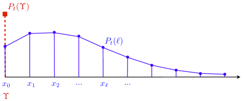
Figure 1: Discretization of the state space as a regular finite grid. Value $y=0$ is either the node $x_{0}$ at which the value of $p_{t}$ is evaluated and the cemetery point $\Upsilon$.

We now derive the finite difference approximation of the continuous part $p_{t}$, returning to the weak formulation. For suitable test function $\phi$,

$$\int_{0}^{\infty}p_{t}(y\,|\,x)\,{\mathcal{A}}\phi(y)\,{{\textrm{d}}}y \simeq\frac{h}{2}\,p_{t}(0\,|\,x)\,{\mathcal{A}}\phi(0)+h\,\sum_{\ell=1}^{L-1}p_{t}(x_{\ell}\,|\,x)\,{\mathcal{A}}\phi(x_{\ell})+\frac{h}{2}\,p_{t}(x_{L}\,|\,x)\,{\mathcal{A}}\phi(x_{L})\$$

$$\simeq\sum_{\ell=0}^{L}P_{t}(l)\,{\mathcal{A}}\phi(x_{\ell})$$

with

$$P_{t}(0)\simeq\frac{h}{2}\,p_{t}(0\,|\,x),\quad P_{t}(L)\simeq\frac{h}{2}\,p_{t}(x_{L}\,|\,x),\quad P_{t}(\ell)\simeq h\,p_{t}(x_{\ell}\,|\,x),\,\text{ for }0<\ell<L\,.$$ (11)

We also need to define $P_{t}(\Upsilon)\simeq E_{t}(x)$. When designing our approximation, we expect $P_{t}(\cdot)$ to be a discrete probability distribution on $\{\Upsilon,x_{0},\dots,x_{L}\}$. The differential operator ${\mathcal{A}}$ is now replaced by its finite difference approximation, denoted $A$, using an up–wind scheme, which reads for an interior point $x_{\ell}$ with $1\leq\ell\leq L-1$:

$$\phi^{\prime}(x_{\ell}) \simeq\begin{dcases}\frac{\phi(x_{\ell+1})-\phi(x_{\ell})}{h},\quad\text{if }b(x_{\ell})\geq 0\,,\\ \frac{\phi(x_{\ell})-\phi(x_{\ell-1})}{h},\quad\text{if }b(x_{\ell})<0\,,\\ \end{dcases}$$

$$\phi^{\prime\prime}(x_{\ell}) \simeq\frac{\phi(x_{\ell+1})-2\,\phi(x_{\ell})+\phi(x_{\ell-1})}{h^{2}}\,.$$

The resulting approximation can be written as

$${\mathcal{A}}\,\phi(x_{\ell})\simeq A_{\ell,\ell-1}\,\phi(x_{\ell-1})+A_{\ell,\ell}\,\phi(x_{\ell})+A_{\ell,\ell+1}\,\phi(x_{\ell+1}),\quad\ell=1,\dots,(L-1)\,,$$

with

$$\forall\,\ell=1,\dots,L-1,\quad A_{\ell,\ell-1} =\frac{b^{-}(x_{\ell})}{h}+\frac{a(x_{\ell})}{2\,h^{2}}\,,$$

$$A_{\ell,\ell} =-\frac{|b(x_{\ell})|}{h}-\frac{a(x_{\ell})}{h^{2}}\,,$$

$$A_{\ell,\ell+1} =\frac{b^{+}(x_{\ell})}{h}+\frac{a(x_{\ell})}{2\,h^{2}}\,.$$

Appropriate boundary condition at $x_{0}$ and $x_{L}$ will be given later on. It is enlightening to interpret this operator $A$ as the infinitesimal generator of a pure jump Markov process on the grid $(\Upsilon,x_{0},\dots,x_{L})$. Indeed, the extra–diagonal terms of $A$, considered as a matrix, are non–negative and the sum on each row is $0$. $P_{t}(\ell)$ is then the probability that this process occupies site $x_{\ell}$ at time $t$. From an interior point $x_{\ell}$, this process jumps to one of its neighbors with a bias directed according to the drift. This interpretation suggests how to complete the three lines of $A$ not yet defined. We set all coefficient of the first line to $0$, since it corresponds to the absorbing state $\Upsilon$. We introduce the notation $\mathbf{P}_{t}=\left(P_{t}(\ell)\right)_{\ell=\Upsilon,0,\dots,L}$ for the law of the jump process at time $t$ starting from $x$. This probability distribution solves the Fokker–Planck equation for jump processes that reads

$$\dot{\mathbf{P}}_{t}=A^{\ast}\mathbf{P}_{t}\ .$$ (12)

Observe that the first ODE of system (12) is

$$\dot{P}_{t}(0)=A_{0,0}\,P_{t}(0)+A_{1,0}\,P_{t}(1)$$

where

$$A_{1,0}=\frac{b^{-}(h)}{h}+\frac{a(h)}{2\,h^{2}}\,.$$

Using (11), this gives an approximation

$$\frac{\partial p_{t}(0\,|\,x)}{\partial t}\simeq\left(2\,\frac{b^{-}(h)}{h}+\frac{a(h)}{h^{2}}\right)\,p_{t}(h\,|\,x)+A_{0,0}\,p_{t}(0\,|\,x)\,.$$ (13)

A suggestion is to find $A_{0,0}$ such that (13) is a finite difference approximation for $\lim_{y\downarrow 0}{\mathcal{A}}^{\ast}p_{t}(y\,|\,x)$:

$$\lim_{y\downarrow 0}{\mathcal{A}}^{\ast}p_{t}(y\,|\,x) =-b^{\prime}(0)\,p_{t}(0\,|\,x)+\frac{1}{2}\,a^{\prime\prime}(0)\,p_{t}(0\,|\,x)+\frac{\partial p_{t}(y\,|\,x)}{\partial y}{\Big{|}_{y=0}}\ a^{\prime}(0)\,.$$

This limit involves only the first derivative of $p_{t}(y\,|\,x)$ due to the vanishing diffusion. With

$$\frac{\partial p_{t}(y\,|\,x)}{\partial y}{\Big{|}_{y=0}}\simeq\frac{p_{t}(h\,|\,x)-p_{t}(0\,|\,x)}{h}$$

we obtain the approximation

$$\frac{\partial p_{t}(0\,|\,x)}{\partial t} \simeq p_{t}(0\,|\,x)\,\left[-b^{\prime}(0)+\frac{1}{2}\,a^{\prime\prime}(0)-\frac{1}{h}\,a^{\prime}(0)\right]+p_{t}(h\,|\,x)\frac{1}{h}\,a^{\prime}(0)\,.$$ (14)

Using

$$a(h)=h\,a^{\prime}(0)+h^{2}\,\frac{1}{2}\,a^{\prime\prime}(0)$$

in (13) we get

$$\frac{\partial p_{t}(0\,|\,x)}{\partial t}\simeq 2\,\frac{b^{-}(h)}{h}\,p_{t}(h\,|\,x)+p_{t}(h\,|\,x)\frac{1}{h}\,a^{\prime}(0)+\frac{1}{2}\,a^{\prime\prime}(0)\,p_{t}(h\,|\,x)+A_{0,0}\,p_{t}(0\,|\,x)\ .$$

Also, $p_{t}(h\,|\,x)\simeq p_{t}(0\,|\,x)$ gives

$$\frac{\partial p_{t}(0\,|\,x)}{\partial t}\simeq p_{t}(0\,|\,x)\,\left[2\,\frac{b^{-}(h)}{h}+\frac{1}{2}\,a^{\prime\prime}(0)+A_{0,0}\right]+p_{t}(h\,|\,x)\frac{1}{h}\,a^{\prime}(0)\ .$$

Now since

$$b^{-}(h)=\frac{|b(h)|-b(h)}{2}\quad\text{and}\quad b(h)\simeq h\,b^{\prime}(0)$$

we finally have

$$\frac{\partial p_{t}(0\,|\,x)}{\partial t}\simeq p_{t}(0\,|\,x)\,\left[|b^{\prime}(0)|-b^{\prime}(0)+\frac{1}{2}\,a^{\prime\prime}(0)+A_{0,0}\right]+p_{t}(h\,|\,x)\frac{1}{h}\,a^{\prime}(0)\ .$$

In order to have an approximation of (14), we must set

$$A_{0,0}=-|b^{\prime}(0)|-\frac{1}{h}\,a^{\prime}(0)\,.$$

This diagonal term of $A$ is non–negative as expected. We see that the state $0$ of the jump process is not absorbing since $A_{0,0}\not=0$, but act as a transition state towards extinction $\Upsilon$. Since there is no reason to allow a jump to an interior point, we also set

$$\forall\,\ell=1,\dots L\quad A_{0,\,\ell}=0,\quad\text{ and }\quad A_{0,\Upsilon}=-A_{0,0}\ .$$

Observe that, from (12) the probability of extinction $P_{t}(\Upsilon)$ satisfies the evolution equation

$$\dot{P}_{t}(\Upsilon)=-A_{0,0}\,P_{t}(0)=\Big{(}\frac{1}{2}\,a^{\prime}(0)+\frac{h}{2}\,|b^{\prime}(0)|\Big{)}\;p_{t}(0\,|\,x)\,.$$

When $h\downarrow 0$, this equation is consistent with (9a) which gives the rate of extinction. Notice that $A_{0,0}$ could have been chosen so that the above equation exactly matches (9a), but then (13) and (14) would not match so closely.

The right boundary is simple: in order for the jump process to remain on the grid, its behavior at boundary $x_{L}$ has to be prescribed artificially. There is no canonical choice between absorbing or reflecting boundary condition, since both corrupt the theoretical behavior. We choose the reflecting boundary condition at $x_{L}$ that reads:

$$A_{L,L-1} =\frac{|b(x_{L})|}{h}+\frac{a(x_{L})}{h^{2}}\,, A_{L,L} =-\frac{|b(x_{L})|}{h}-\frac{a(x_{L})}{h^{2}}\,.$$

The sum on the last row is $0$, so that there is no probability leak at boundary $x_{L}$. The boundary condition at $0$ requires more care.

Time discretization

Equation (12) is discretized in time using the Euler implicit scheme

$$[I-\delta\,A]^{\ast}\,\mathbf{\tilde{P}}_{t_{k+1}}=\mathbf{\tilde{P}}_{t_{k}}\,,\quad k=0,\dots,n-1$$

where $t_{k}\stackrel{{\scriptstyle{\textrm{\rm\tiny def}}}}{{=}}k\,\delta$ with $\delta=\Delta/n$, $n$ given; see Figure 2. The initial condition is approximated by

$$\tilde{P}_{t_{0}}(l)=\begin{dcases}1\,,&\text{ if }\ell=\ell_{0}\,,\\ 0\,,&\text{ otherwise, }\end{dcases}$$

where $x_{\ell_{0}}$ is the nearest neighbor in the grid of the initial condition $x$. According to (11), the numerical solution $\mathbf{\tilde{P}}_{\Delta}$ yields a numerical approximation $\tilde{p}_{\Delta}(x_{\ell}\,|\,x)$ for the density at a grid point, that can be linearly interpolated to obtain an approximation $\tilde{p}_{\Delta}(y\,|\,x)$ for $0\leq y\leq x_{L}$. The likelihood function is then approximated by

$$q_{\Delta}(x,y)\simeq\begin{dcases}\textstyle P_{\Delta}(\Upsilon)\,,&\text{ if }y=0\,,\\ \tilde{p}_{\Delta}(y\,|\,x)\,,&\textrm{ if }y\in]0,x_{L}]\,.\end{dcases}$$

Figure 2: The observation instants are $t^{\textrm{\rm\tiny o}}_{k}=k\,\Delta$ with $\Delta=\frac{T}{M}$; the time-discretization instants are $t_{k}=k\,\delta$ with $\delta=\frac{\Delta}{n}$ for $n$ given.

Remark 3.1

This discretization scheme is unconditionally stable, but $h$ and $\delta$ have to be chosen in a coherent way. Indeed, $-A(\ell,\ell)$ gives the expectation of the holding time of the pure jump Markov process. We see that the order of magnitude of the holding time is $\frac{1}{h^{2}}$. The time step $\delta$ should then be chosen small enough to ensure that not too many jumps occur within an interval of length $\delta$.

The numerical treatment of the Fokker–Planck equation in the degenerate case has already been considered in the numerical analysis, see for example Cacio et al. [2]. The approach adopted in this work retains the probabilistic meaning of the objects involved, at the cost of a possible loss of accuracy.

3.2 Monte Carlo approximations

A number of estimation methods using Monte Carlo simulations have been proposed in the absolutely continuous case, see Hurn et al. [12] and references therein for a detailed review, or Fearnhead [7] which includes many application examples. In this section, we will design modifications of some of them in order to handle the extinction feature.

The numerical approximations of Monte Carlo type presented hereafter involve simulation of a $N$–samples with common law $Q_{\Delta}^{\theta}({{\textrm{d}}}y\,|\,x)$, for many different initial conditions $x$. In our case, we will not be able to draw random variates from $Q_{\Delta}^{\theta}({{\textrm{d}}}y\,|\,x)$ exactly, but only from distributions close to it. The simplest algorithm for simulating trajectories of (2) is the Euler–Maruyama scheme, restricted to non–negative values, that is

$$\bar{X}_{t_{k+1}} =\max\Big{(}0,\bar{X}_{t_{k}}+\delta\,b(\bar{X}_{t_{k}})+\sqrt{\delta}\,\sigma(\bar{X}_{t_{k}})\,w_{k}\Big{)}\,,\quad k=0,\dots,n-1$$ (15)

with $\bar{X}_{0}=x$ and where $w_{k}$ are i.i.d. ${\mathcal{N}}(0,1)$. One iteration of the approximation scheme (15) amounts to draw from the transition kernel $K_{\delta}({{\textrm{d}}}z\,|\,x)$ instead of $Q_{\delta}({{\textrm{d}}}z\,|\,x)$ where $K_{\delta}({{\textrm{d}}}z\,|\,x)$ is defined by:

$$K_{\delta}({{\textrm{d}}}z\,|\,x)\stackrel{{\scriptstyle{\textrm{\rm\tiny def}}}}{{=}}\begin{cases}e_{\delta}(x)\,\delta_{0}({{\textrm{d}}}z)+g_{\delta}(z\,|\,x)\,{{\textrm{d}}}z\,,&\textrm{ if }x>0\,,\\ \delta_{0}({{\textrm{d}}}z)\,,&\textrm{ if }x=0\,,\end{cases}$$ (16)

with

$$e_{\delta}(x) \stackrel{{\scriptstyle{\textrm{\rm\tiny def}}}}{{=}}\textstyle 1-\int_{0}^{\infty}g_{\delta}(z\,|\,x)\,{{\textrm{d}}}z\,,$$

$$g_{\delta}(z\,|\,x) \stackrel{{\scriptstyle{\textrm{\rm\tiny def}}}}{{=}}\textstyle\frac{1}{\sqrt{2\,\pi\,\delta\,\sigma(x)}}\,\exp\left\{-\frac{(z-x-\delta\,b(x))^{2}}{2\,\delta\,\sigma(x)}\right\}\,\mathbf{1}_{\mathbb{R}_{+}}(z)\,.$$

It is known that this approximation is valid if $\delta$ is sufficiently small, see Risken [19, chapter 4]. The numerical scheme (15) produces samples of common law $Q^{\textrm{\tiny E}}_{\Delta}({{\textrm{d}}}y\,|\,x)$

$$Q^{\textrm{\tiny E}}_{\Delta}({{\textrm{d}}}y\,|\,x)=\int_{\{y_{1}\geq 0\}}\cdots\int_{\{y_{n-1}\geq 0\}}K_{\delta}({{\textrm{d}}}y_{1}\,|\,x)\,K_{\delta}({{\textrm{d}}}y_{2}\,|\,y_{1})\,\cdots K_{\delta}({{\textrm{d}}}y\,|\,y_{n-1})\ ,$$ (17)

which is an approximation of the true transition kernel $Q_{\Delta}({{\textrm{d}}}y\,|\,x)$. Notice that, using the semi–group and the Markov properties, we also have a similar decomposition

$$Q_{\Delta}({{\textrm{d}}}y\,|\,x)=\int_{\{y_{1}\geq 0\}}\cdots\int_{\{y_{n-1}\geq 0\}}Q_{\delta}({{\textrm{d}}}y_{1}\,|\,x)\,Q_{\delta}({{\textrm{d}}}y_{2}\,|\,y_{1})\,\cdots Q_{\delta}({{\textrm{d}}}y\,|\,y_{n-1})\ .$$

Remark 3.2

The recent works Beskos and Roberts [1] about the Exact Algorithm (EA) seems promising for drawing exactly from $Q_{\Delta}({{\textrm{d}}}y\,|\,x)$. To our knowledge, this algorithm cannot be applied directly to our specific case, due to the almost sure extinction. There are also other alternatives to (15), such as the Milstein scheme, see e.g. Kloeden et al. [16], or Euler–Maruyama scheme for killed diffusion, see Gobet [9]. Modifications of these algorithms might be necessary to cope with the extinction problem.

Remark 3.3

If $\Delta$ is itself small enough, there would be no need to simulate the solution of (2) at intermediate time between $0$ and $\Delta$, since $K_{\Delta}$ has an explicit density with respect to $m$. However, for most applications, the observations are not available at a so high sampling rate.

3.2.1 Non–parametric estimation

A simple usage of the approximation scheme (15) is to produce a $N$–sample $\bar{X}_{\Delta}^{(1)},\dots\bar{X}_{\Delta}^{(N)}$ of $Q^{\textrm{\tiny E}}_{\Delta}({{\textrm{d}}}y\,|\,x)$. These faked observations are then fed into a nonparametric estimate of the density $p_{\Delta}(y\,|\,x)$ at $y$, denoted by $\hat{p}_{\Delta}(y\,|\,x)$. Again, the case of extinction should be cared for by first discarding the values $\bar{X}_{\Delta}^{(i)}=0$, if there are any, from the estimation. The resulting approximation reads

$$q_{\Delta}(y\,|\,x)\simeq\begin{cases}\frac{N-N_{s}}{N}\,,&\text{ if }y=0\,,\\ \frac{N_{s}}{N}\,\hat{p}_{\Delta}(y\,|\,x)\,,&\text{ otherwise }\end{cases}$$

where $N_{s}$ is the random number of trajectories still alive at time $\Delta$, that is

$$N_{s}\stackrel{{\scriptstyle{\textrm{\rm\tiny def}}}}{{=}}\#\big{\{}i=1,\dots,N\,;\,\bar{X}_{\Delta}^{(i)}\neq 0\big{\}}\,.$$

This approach, without extinction, is presented in Hurn et al. [11]. Its efficiency relies on that of the nonparametric estimation method used and is therefore subject to the classical problems of choice of bandwidth and leakage of mass in inaccessible region ($\mathbb{R}_{-}$ in our case).

3.2.2 Pedersen method

Figure 3: The Perdersen approximation $Q^{\textrm{\tiny P}}_{\Delta}$ of the kernel $Q_{\Delta}$ is obtained by sampling $N$ independent trajectories $\bar{X}_{t_{0:n-1}}^{(i)}$ from (15); then the approximation is given by (19). See text for the precise treatment of extinct trajectories.

It is possible to avoid the non–parametric estimation stage. Indeed from the Markov property:

$$Q_{\Delta}({{\textrm{d}}}y\,|\,x)=(Q_{\Delta-\delta}Q_{\delta})({{\textrm{d}}}y\,|\,x)=\int_{\{y_{n-1}\geq 0\}}Q_{\Delta-\delta}({{\textrm{d}}}y_{n-1}\,|\,x)\,Q_{\delta}({{\textrm{d}}}y\,|\,x)\,,$$ (18)

first approximate $Q_{\Delta-\delta}({{\textrm{d}}}y_{n-1}\,|\,x)$ by $Q^{\textrm{\tiny E}}_{\Delta-\delta}({{\textrm{d}}}y_{n-1}\,|\,x)$, hence

$$Q_{\Delta-\delta}({{\textrm{d}}}y_{n-1}\,|\,x)\simeq\frac{1}{N}\,\sum_{i=1}^{N}\delta_{\bar{X}_{t_{n-1}}^{(i)}}({{\textrm{d}}}y_{n-1})$$

where $\bar{X}_{t_{n-1}}^{(i)}\stackrel{{\scriptstyle\textrm{iid}}}{{\sim}}Q^{\textrm{\tiny E}}_{\Delta-\delta}({{\textrm{d}}}y_{n-1}\,|\,x)$, $i=1,\dots,N$; then approximating $Q_{\delta}({{\textrm{d}}}y\,|\,y_{n-1})$ by $K_{\delta}({{\textrm{d}}}y\,|\,y_{n-1})$, leads to the following approximation of the kernel $Q_{\Delta}({{\textrm{d}}}y\,|\,x)$:

$$Q^{\textrm{\tiny P}}_{\Delta}({{\textrm{d}}}y\,|\,x) \stackrel{{\scriptstyle{\textrm{\rm\tiny def}}}}{{=}}\frac{1}{N}\,\sum_{i=1}^{N}K_{\delta}({{\textrm{d}}}y\,|\,\bar{X}_{t_{n-1}}^{(i)})$$ (19)

see Figure 3. Let us re–numbered the sampled trajectories so that the surviving ones correspond to $i=1,\dots,N_{s}$, according to (16) we get:

$$Q^{\textrm{\tiny P}}_{\Delta}({{\textrm{d}}}y\,|\,x) =\textstyle\frac{1}{N}\,\sum_{i=N_{s}+1}^{N}K_{\delta}({{\textrm{d}}}y\,|\,0)+\frac{1}{N}\,\sum_{i=1}^{N_{s}}K_{\delta}({{\textrm{d}}}y\,|\,\bar{X}_{t_{n-1}}^{(i)})$$

$$=\textstyle\frac{N-N_{s}}{N}\,\delta_{0}({{\textrm{d}}}y)+\frac{1}{N}\,\sum_{i=1}^{N_{s}}\big{[}e_{\delta}(\bar{X}_{t_{n-1}}^{(i)})\,\delta_{0}({{\textrm{d}}}y)+g_{\delta}(y\,|\,\bar{X}_{t_{n-1}}^{(i)})\,{{\textrm{d}}}y\big{]}$$

$$=\textstyle\big{[}\frac{N-N_{s}}{N}+\frac{1}{N}\,\sum_{i=1}^{N_{s}}e_{\delta}(\bar{X}_{t_{n-1}}^{(i)})\big{]}\,\delta_{0}({{\textrm{d}}}y)+\frac{1}{N}\,\sum_{i=1}^{N_{s}}g_{\delta}(y\,|\,\bar{X}_{t_{n-1}}^{(i)})\,{{\textrm{d}}}y$$

so that $Q^{\textrm{\tiny P}}_{\Delta}({{\textrm{d}}}y\,|\,x)$ admits the following density with respect to the measure $m({{\textrm{d}}}y)$:

$$q^{\textrm{\tiny P}}_{\Delta}(y\,|\,x)\stackrel{{\scriptstyle{\textrm{\rm\tiny def}}}}{{=}}\begin{cases}\displaystyle\frac{N-N_{s}}{N}+\frac{1}{N}\,\sum_{i=1}^{N_{s}}e_{\delta}(\bar{X}_{t_{n-1}}^{(i)})\,,&\text{ if }y=0\,,\\ \displaystyle\frac{1}{N}\,\sum_{i=1}^{N_{s}}g_{\delta}(y\,|\,\bar{X}_{t_{n-1}}^{(i)})\,,&\text{ otherwise. }\end{cases}$$

This approach is presented in Pedersen [18] for diffusion on $\mathbb{R}^{d}$ having an absolutely continuous density. Even with our adaptation allowing the extinction, it is very easy to implement and does not involve heavy computations. It suffers however from a well known problem of Monte Carlo methods: if not so many trajectories terminate around the observation $y$ at which the density is to be evaluated, then only a few terms will significantly contribute to the approximation of $p_{\Delta}({{\textrm{d}}}y\,|\,x)$. In this case the approximation will be of poor quality. Beside, a number of trajectories will have been generated uselessly. This problem is usually well tackled by importance sampling procedures.

3.2.3 Importance sampling with a Brownian bridge

Figure 4: The approximation $Q^{\textrm{\tiny B}}_{\Delta}$ by importance sampling with a Brownian bridge of the kernel $Q_{\Delta}$ is obtained by sampling $N$ independent trajectories $\tilde{X}_{t_{0:n-1}}^{(i)}$ of the approximation of the Brownian bridge (20); then the approximation is given by (23). See text for the precise treatment of extinct trajectories.

When using importance sampling, the trajectories from $x$ to $y_{n-1}$ are sampled according to a different process and weighted to correct the change of law. Such a procedure is described among others in Durham and Gallant [5]. Once again, we have to modify the method to account for the possible extinction. Our choice is to generate the trajectories according to

$$\tilde{X}_{t_{k+1}}=\max\Big{(}0,\tilde{X}_{t_{k}}+\delta\,\frac{y-\tilde{X}_{t_{k}}}{\Delta-{t_{k}}}+\sqrt{\delta}\,\sigma(\tilde{X}_{t_{k}})\,w_{k}\Big{)}\,,\quad k=0,\dots,n-1$$ (20)

whith $X_{0}=x$ and $w_{k}\stackrel{{\scriptstyle\textrm{iid}}}{{\sim}}{\mathcal{N}}(0,1)$ which is nothing but a (modified for extinction) Euler–Maruyama scheme for the SDE

$${{\textrm{d}}}X_{t}=\frac{y-X_{t}}{\Delta-t}\,{{\textrm{d}}}t+\sigma(X_{t})\,{{\textrm{d}}}W_{t},\quad 0\leq t<\Delta\,.$$ (21)

The drift term is designed so as to force the trajectories towards the given final value $y$. Note that solution of (21) would be a “true” Brownian bridge if $\sigma$ were constant. The transition kernel associated with (20) depends on $t<\Delta$ and reads:

$$\tilde{K}_{t,\delta}({{\textrm{d}}}z\,|\,x)=\begin{cases}\tilde{e}_{\delta}(x)\,\delta_{0}({{\textrm{d}}}z)+\tilde{g}_{t,\delta}(z\,|\,x)\,{{\textrm{d}}}z\,,&\textrm{if }x>0\,,\\ \delta_{0}({{\textrm{d}}}z)\,,&\textrm{if }x=0\,,\end{cases}$$ (22)

where

$$\tilde{e}_{\delta}(x) \stackrel{{\scriptstyle{\textrm{\rm\tiny def}}}}{{=}}\textstyle\left(1-\int_{0}^{\infty}\tilde{g}_{t,\delta}(z\,|\,x)\,{{\textrm{d}}}z\right)\,,$$

$$\tilde{g}_{t,\delta}(z\,|\,x) \stackrel{{\scriptstyle{\textrm{\rm\tiny def}}}}{{=}}\textstyle\frac{1}{\sqrt{2\,\pi\,\delta\,\sigma(x)}}\,\exp\Big{\{}-\frac{(z-x-\delta\,\frac{y-x}{\Delta-t})^{2}}{2\,\delta\,\sigma(x)}\Big{\}}\,\mathbf{1}_{\mathbb{R}_{+}}(z)\,.$$

This transition kernel is absolutely continuous with respect to $K_{\delta}({{\textrm{d}}}z\,|\,x)$:

$$\tilde{K}_{\delta}({{\textrm{d}}}z\,|\,x)=\psi_{t,\delta}(z\,|\,x)\,K_{t,\delta}({{\textrm{d}}}z\,|\,x)$$

with

$$\psi_{t,\delta}(z\,|\,x) =\begin{dcases}\frac{1-\int_{0}^{\infty}g_{\delta}(z\,|\,x)\,{{\textrm{d}}}z}{1-\int_{0}^{\infty}\tilde{g}_{t,\delta}(z\,|\,x)\,{{\textrm{d}}}z}\,,&\text{ if }z=0\,,\\[3.00003pt] \displaystyle\frac{\int_{0}^{\infty}g_{\delta}(z\,|\,x)\,{{\textrm{d}}}z}{\int_{0}^{\infty}\tilde{g}_{t,\delta}(z\,|\,x)\,{{\textrm{d}}}z}\,,&\text{ otherwise, }\end{dcases}$$

for $x>0$ and $\psi_{t,\delta}(z\,|\,0)=\mathbf{1}_{\mathbb{R}_{+}}(z)$. We now have another expression for $Q^{\textrm{\tiny E}}_{\Delta-\delta}({{\textrm{d}}}y_{n-1}\,|\,x)$ as

$$Q^{\textrm{\tiny E}}_{\Delta-\delta}({{\textrm{d}}}y_{n-1}\,|\,x)=\int_{0}^{\infty}\dots\int_{0}^{\infty}\Psi(y_{1},\dots,y_{n-1}\,|\,x)\,\tilde{K}_{0,\delta}({{\textrm{d}}}y_{1}\,|\,x)\dots\tilde{K}_{\Delta-2\,\delta,\delta}({{\textrm{d}}}y_{n-1}\,|\,y_{n-2})$$

where

$$\Psi(y_{1},\dots,y_{n-1}\,|\,x)=\psi_{\delta,\delta}(y_{1}\,|\,x)\dots\psi_{\Delta-2\,\delta,\delta}(y_{n-1}\,|\,y_{n-2})\,.$$

Hereafter, we will denote by

$$\tilde{X}_{t_{1:n-1}}=(\tilde{X}_{t_{1}},\dots,\tilde{X}_{t_{n-1}})\in\mathbb{R}^{n}$$

a trajectory generated by (20) up to time $\Delta-\delta$, with initial value $\tilde{X}_{0}=x$.

With this setting, and like in the previous section, in (18) first approximate $Q_{\Delta-\delta}$ by a weighted sample

$$Q_{\Delta-\delta}({{\textrm{d}}}y_{n-1}\,|\,x)\simeq\frac{1}{N}\,\sum_{i=1}^{N}\Psi(\tilde{X}_{t_{1:n-1}}^{(i)}\,|\,x)\,\delta_{\tilde{X}_{t_{n-1}}^{(i)}}({{\textrm{d}}}y_{n-1})$$

then, as before, approximate $Q_{\delta}({{\textrm{d}}}y\,|\,y_{n-1})$ by $K_{\delta}({{\textrm{d}}}y\,|\,y_{n-1})$; finally the kernel $Q_{\Delta}({{\textrm{d}}}y\,|\,x)$ defined by (18) is approximated by:

$$Q^{\textrm{\tiny B}}_{\Delta}({{\textrm{d}}}y\,|\,x) \stackrel{{\scriptstyle{\textrm{\rm\tiny def}}}}{{=}}\frac{1}{N}\,\sum_{i=1}^{N}\Psi(\tilde{X}_{t_{1:n-1}}^{(i)}\,|\,x)\,K_{\delta}({{\textrm{d}}}y\,|\,\tilde{X}_{t_{n-1}}^{(i)})\,.$$ (23)

As before, let us re–numbered the sampled trajectories so that the surviving ones correspond to $i=1,\dots,N_{s}$:

$$Q^{\textrm{\tiny B}}_{\Delta}({{\textrm{d}}}y\,|\,x) =\textstyle\frac{1}{N}\,\sum_{i=N_{s}+1}^{N}\Psi(\tilde{X}_{t_{1:n-1}}^{(i)}\,|\,x)\,K_{\delta}({{\textrm{d}}}y\,|\,0)+\frac{1}{N}\,\sum_{i=1}^{N_{s}}\Psi(\tilde{X}_{t_{1:n-1}}^{(i)}\,|\,x)\,K_{\delta}({{\textrm{d}}}y\,|\,\tilde{X}_{t_{n-1}}^{(i)})$$

$$=\textstyle\frac{1}{N}\,\sum_{i=N_{s}+1}^{N}\Psi(\tilde{X}_{t_{1:n-1}}^{(i)}\,|\,x)\,\delta_{0}({{\textrm{d}}}y)$$

$$\textstyle\qquad\qquad+\frac{1}{N}\,\sum_{i=1}^{N_{s}}\Psi(\tilde{X}_{t_{1:n-1}}^{(i)}\,|\,x)\,\big{[}e_{\delta}(\tilde{X}_{t_{n-1}}^{(i)})\,\delta_{0}({{\textrm{d}}}y)+g_{\delta}(y\,|\,\tilde{X}_{t_{n-1}}^{(i)})\,{{\textrm{d}}}y\big{]}$$

$$=\textstyle\big{[}\frac{1}{N}\,\sum_{i=N_{s}+1}^{N}\Psi(\tilde{X}_{t_{1:n-1}}^{(i)}\,|\,x)+\frac{1}{N}\,\sum_{i=1}^{N_{s}}\Psi(\tilde{X}_{t_{1:n-1}}^{(i)}\,|\,x)\,e_{\delta}(\tilde{X}_{t_{n-1}}^{(i)})\big{]}\,\delta_{0}({{\textrm{d}}}y)$$

$$\textstyle\qquad\qquad+\frac{1}{N}\,\sum_{i=1}^{N_{s}}\Psi(\tilde{X}_{t_{1:n-1}}^{(i)}\,|\,x)\,g_{\delta}(y\,|\,\tilde{X}_{t_{n-1}}^{(i)})\,{{\textrm{d}}}y$$

hence $Q^{\textrm{\tiny B}}_{\Delta}({{\textrm{d}}}y\,|\,x)$ admits the following density with respect to $m({{\textrm{d}}}y)$:

$$q^{\textrm{\tiny B}}_{\Delta}(y\,|\,x)\stackrel{{\scriptstyle{\textrm{\rm\tiny def}}}}{{=}}\begin{dcases}\frac{1}{N}\,\sum_{i=N_{s}+1}^{N}\Psi(\tilde{X}_{t_{1:n-1}}^{(i)}\,|\,x)+\frac{1}{N}\,\sum_{i=1}^{N_{s}}\Psi(\tilde{X}_{t_{1:n-1}}^{(i)}\,|\,x)\,e_{\delta}(\tilde{X}_{t_{n-1}}^{(i)})\,,&\text{ if }y=0\,,\\ \frac{1}{N}\,\sum_{i=1}^{N_{s}}\Psi(\tilde{X}_{t_{1:n-1}}^{(i)}\,|\,x)\,g_{\delta}(y\,|\,\tilde{X}_{t_{n-1}}^{(i)})\,,&\text{ otherwise. }\end{dcases}$$

Remark 3.4

It is possible to use other importance sampler than (20). Durham and Gallant [5] use a modified Brownian bridge which seems to reduce further the variance of the resulting approximation. The generating algorithm reads

$$\tilde{X}_{t_{k+1}}=\tilde{X}_{t_{k}}+\delta\,\frac{y-\tilde{X}_{t_{k}}}{\Delta-t}+\sqrt{\delta}\,\sigma(\tilde{X}_{t_{k}})\,(1-\frac{\delta}{\Delta-t})\,w_{k}\,.$$

The drift term is as in (20) but the variance is progressively damped up to final time $t=\Delta-2\,h$ at which it equals $\frac{1}{2}\,\sigma(Y_{t})$.

4 Numerical experiments

We now evaluate the numerical performance of the approximation methods described above, on the scenario defined by the model parameter given in Table 1. These values are chosen so as to observe a short transient phase where the population grows quickly, starting from a small initial value, and a stationary phase with a high noise intensity. The simulation parameters of the approximation methods are also given by Table 1. In particular, the same time step $\delta$ is used for all methods.

Model
$\lambda$	$\mu$	$\alpha$	$\rho$	$x_{0}$	$T$	$N$
$20$	$18$	$1$	$10^{-1}$	0.25	10	200

Simulation
$h$	$\delta$	$N$
$10^{-3}$	$10^{-3}$	$200$

Table 1: Parameters

4.1 Dynamics

Figure 5 shows 200 trajectories of model (2), simulated with the Euler–Maruyama scheme. Within the time interval of the simulation, we observe the three possible behaviors:

• Early extinction during the transient phase. This stems from the fact that the initial level of the population is small and the noise intensity is high.

• Completed transient phase followed by noisy fluctuations around a natural carrying capacity. Even if it is known that all trajectories will eventually reach 0, all of them but one survive on the short term.

• Late extinction after reaching the stationary phase. Only one trajectory is concerned.

Due to early extinction, the estimated extinction probability grows quickly in the first part, and seems to approach an asymptotic value. Running the simulation on a much larger period of time will result in an extinction frequency reaching $1$ slowly. This Figure is to be compared with Figure 6 showing a contour plot of the numerical solution of Fokker–Planck equation (9) obtained by implementing the finite difference scheme of section 3.1. As expected, the first two moments quickly move to stationary values, after a transient phase where a large amount of mass is lost. On the long term, the mass keeps on decreasing slowly.

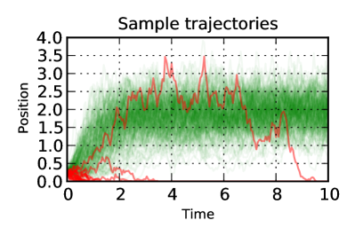
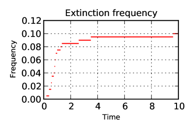
Figure 5: On the left: simulation of $n=200$ trajectories according to dynamics (2). Trajectories in red become extinct before final time. One of them completes the transient phase. On the right plot, the corresponding extinction frequency.

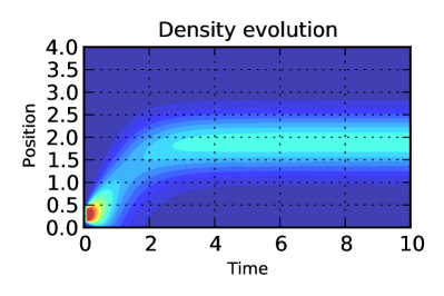
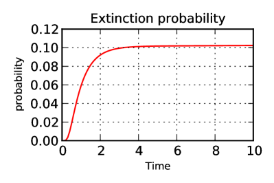
Figure 6: Finite difference approximation of Fokker–Planck equation (9). Diffusion induces a quick loss of mass in the transient phase. The loss of mass is then much slower.

4.2 Kernel approximations

We now investigate the ability of the methods to approximate the density $q_{\Delta}$, since the final parameter estimation heavily relies on the quality of this approximation. For this section, we take $T=1$ in order to observe correctly both continuous and discrete parts of $q_{\Delta}$. The other parameters are unchanged. The results obtained with the finite difference method are shown on the top row of Figure 7. There is no way to evaluate its performance since the exact solution is not available. However, the picture presented here does not change significantly when we use smaller discretization steps.

To compare with the Monte Carlo methods, we consider the extinction probability $E_{\Delta}$ together with the value of the continuous part $p_{\Delta}(x,y)$ at three locations $y_{1},\,y_{2}$ and $y_{3}$. The bottom line of Figure 7 shows the results of 200 independent realizations of the two Monte Carlo methods. The green dashed line gives the values obtained by finite difference approximation. As expected, the variance observed for the modified Brownian bridge is much smaller than for the Pedersen method. However the computational cost needed to achieve this performance is high. It is worth remembering also that the $N$ trajectories simulated for the Pedersen method do not depend of the value at which the density is evaluated. A single run of a $N$ path allows the estimation of the density at any point. This is not the case for the modified Brownian bridge method for which a new run is needed for each terminal value. Finally, we note that, even for the modified Brownian bridge method, we observe a large number of outliers which are likely to corrupt the final evaluation of the likelihood.

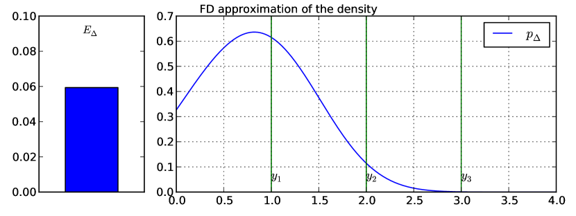
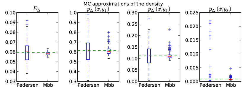
Figure 7: Comparison of approximation methods for the approximation of the density which solves equation (9). The top row shows the finite difference approximation of the density $q_{\Delta}$. The left plot is the discrete component and the right plot shows the continuous one. The four plots on the bottom rows give the Monte Carlo approximations of the density at four different locations. The green horizontal dashed line is the value given by the finite difference approximation. The model parameters are given in Table 1, except for $\Delta=1$. The box–plots are based on $200$ realizations. Both Monte Carlo methods use $N=500$ particles.

4.3 Likelihood approximations

The numerical results presented in this section are based on a typical trajectory of Figure 5. We obtain the set of data by sampling the trajectory at instants $k\,\Delta$, for $k=0,\dots,200$ and $\Delta=0.05$. We take $\theta=(\lambda,\mu)\in\mathbb{R}^{2}_{+}$ as our parameter to be estimated and the other model parameters $\alpha$, $\kappa$ as fixed known values. The initial condition $x_{0}$ is also deterministic and known. To improve numerical stability, we will note $\ell(\theta)=-\log({\mathcal{L}}(\theta))$ and study the minimum of $\ell(\theta)$. Figure 8 shows the graph of the finite difference approximation of the function to minimize $\ell(\theta)$. We clearly distinguish two orthogonal directions of variations defined respectively by the equations

$$\lambda+\mu=b,\quad\text{ and }\quad\lambda-\mu=b^{\prime}\ .$$

Along the first direction, $\ell(\theta)$ decreases rapidly to a local unique minimum. The plot scale needs to be adapted in order to see that a local unique minimum also exists along the second axis, although the variations of $\ell(\theta)$ are much smaller along this axis. It is therefore expected that any iterative minimization algorithm will be directed rapidly to small values of $\ell(\theta)$ along the first axis. Reaching the global minimum by progressing along the second axis will take much more steps. Moreover, it will also require a precise evaluation of the increments of $\ell(\theta)$ between two neighboring values. We are then led to focus on the variance of the values given by the Monte Carlo methods. Figure 9 shows box–plots of  $200$ evaluations of both methods at three different locations. Again we find that the Brownian bridge method performs much better that the Pedersen method, but both of them exhibit random fluctuations with an order of magnitude noticeably greater than the variation of $\ell(\theta)$ along the second axis.

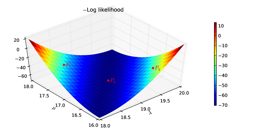
Figure 8: Finite difference approximation of $\ell(\theta)$. The model parameters are given in Table 1. Initial condition is a Dirac mass at $x_{0}=0.25$. The Monte Carlo approximations will be evaluated at points $P_{1},\,P_{2}$ and $P_{3}$.

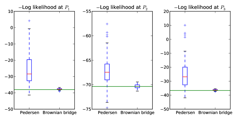
Figure 9: Comparison of Monte Carlo approximations of $\ell(\theta)$ at point $P_{1}$, $P_{2}$ and $P_{3}$ of Figure 8. The box–plots are based on $200$ realizations. Both Monte Carlo methods use $N=500$ particles.

4.4 Estimation results

As noticed in the previous section, the random fluctuations of the Monte Carlo methods will mislay the iterative minimization algorithm. The estimated value returned will be a local minimum, depending essentially on the initial condition and the stopping criterion. The estimation results of this section will then use the finite difference approximation. On Figure 10, we plot the estimated values for the data of Figure 5. We again notice the asymmetry of the empirical distribution of the MLE. The variance is much smaller along the second axis, which means that information on $(\lambda-\mu)$ in the data is better understood than information on $(\lambda+\mu)$. In model (2), the drift coefficient depends on $(\lambda-\mu)$ whereas the diffusion coefficient depends on $(\lambda+\mu)$. In our case, inferring on the diffusion appears to be the hardest task.

Finally, we observe the bad quality of the estimation when the data is a trajectory for which extinction happens during the transient phase. Indeed, even if we have taken good care of the extinction problem, the information given by the data is not sufficient to allow a useful inference on the parameter. On the other hand, the estimation is correct if the observed trajectory reaches the stationary phase, even if extinction occurs later on.

Computational issues.

The results presented herein have been obtained with a C++ code using NLopt nonlinear-optimization package of Steven G. Johnson, freely available at http://ab-initio.mit.edu/nlopt++ which provides the implementation of various algorithms. We have chosen to use a variant of the Nelder and Mead simplex algorithm described in Rowan [20].

Acknowledgements.

This work was partially supported by the Laboratory of Excellence (Labex) NUMEV (Digital and Hardware Solutions, Modelling for the Environment and Life Sciences) coordinated by University of Montpellier 2, France.

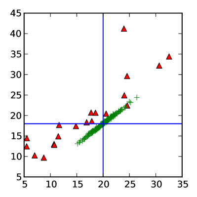
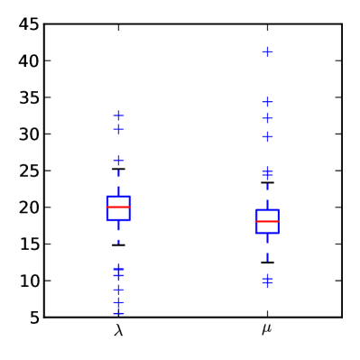
Figure 10: Empirical distribution of the MLE, using the finite difference approximation and parameters of Table 1. The right plot shows the marginal distribution. On the left plot, the red triangles correspond to trajectories becoming extinct before final time, see Figure 5. Late extinction (the red triangle among green crosses) does not affect the estimation

5 Concluding remarks

The parameter estimation problem for a discretely observed diffusion subject to almost sure extinction has been studied. In most practical situations, the observed trajectory does not reach extinction. Indeed, if $\lambda>\mu$, $\rho$ is small and $X_{0}$ is sufficiently large, the mass absorbed at $0$ is negligible, so that the transition kernel is essentially $p_{\Delta}^{\theta}(y\,|\,x)\,{{\textrm{d}}}y$. Nonetheless, it makes sense to take care of the extinction probability $E_{\Delta}(x)$ since the two parts are strongly related. Any maximization algorithm will evaluate this likelihood for many values of the parameter. For some of these values, neglecting the extinction could lead to an abnormally high value of the likelihood and thus mislay the maximization algorithm. Coupling extinction and non–extinction in the complete Fokker–Planck equation results in a more robust estimation procedure. This approach is not specific to the particular application under consideration.

Beyond the extinction problem and separate from it, the identifiability of the parameters is also central in the model presented here. With numerical experiments, we have seen that the transport dynamics, given by the drift coefficient brings only a partial information which does not allow to discriminate clearly between the parameters values. The information on the demographic noise encapsulated in the diffusion coefficient completes the information, although it is much more difficult to extract from the data. The Monte Carlo methods presented here are not able to achieve the precision level required to that end.

Appendix

Appendix A Derivation of the stochastic logistic model (2)

A natural way to derive the SDE (2) is to consider, at a microscopic scale, a population size $N_{t}$ subject to a birth and death process that features a logistic mechanism, e.g.:

$$\mathbb{P}(N_{t+h}=n^{\prime}|N_{t}=n)\displaystyle\mathop{\simeq}_{h\to 0}\begin{cases}h\,\lambda\,n+o(h)\,,&\textrm{if }n^{\prime}=n+1\,,\\ \textstyle h\,(\mu+\frac{\alpha}{\kappa}\,n)\,n+o(h)\,,&\textrm{if }n^{\prime}=n-1\,,\\ \textstyle 1-h\,(\lambda+\mu+\frac{\alpha}{\kappa}\,n)\,n+o(h)\,,&\textrm{if }n^{\prime}=n\,,\\ o(h)\,,&\textrm{otherwise}\end{cases}$$ (24)

with $\lambda>0$, $\mu>0$, $\alpha>0$, $\kappa>0$; here the birth per capita rate $\lambda$ is constant and the death per capita rate $\mu+\frac{\alpha}{\kappa}\,n$ increases linearly with the population size $n$.

The rescaled process:

$$X^{\kappa}_{t}\stackrel{{\scriptstyle{\textrm{\rm\tiny def}}}}{{=}}\frac{1}{\kappa}\,N_{t}$$

is a pure jump Markov process with values in $\frac{1}{\kappa}\,\mathbb{N}$ where $\kappa$ denotes the order of magnitude of the population size $N_{t}$ of interest. The rescaled process is a pure jump Markov process and its distribution law is characterized by its infinitesimal generator:

$$\lim_{t\to 0}\textstyle\frac{\mathbb{E}(\phi(X^{\kappa}_{t})|X^{\kappa}_{0}=x)-\phi(x)}{t}=\lambda\,x\,\left[\phi(x+\frac{1}{\kappa})-\phi(x)\right]+(\mu+\alpha\,x)\,x\,\left[\phi(x-\frac{1}{\kappa})-\phi(x)\right]$$

defined for any bounded function $\phi$. In large population scale, that is for $\kappa$ large, a diffusion approximation of $X^{\kappa}_{t}$ is obtained by performing a second order Taylor expansion of regular functions $\phi$. This yields the operator ${\mathcal{A}}$ defined by (7), which is the infinitesimal generator of the diffusion process solution of (2).

Note that (2) can be rewritten as

$${{\textrm{d}}}X_{t}=r\,\left(1-\frac{X_{t}}{K}\right)\,X_{t}\,{{\textrm{d}}}t+\rho\,\sqrt{r^{\prime}\,\left(1+\frac{X_{t}}{K^{\prime}}\right)\,X_{t}}\,{{\textrm{d}}}B_{t}$$

with $r=\lambda-\mu,$ $K=\frac{r}{\alpha}$, $r^{\prime}=\lambda+\mu$, $K^{\prime}=\frac{r^{\prime}}{\alpha}$ and $\rho=\frac{1}{\sqrt{\kappa}}$, so that its instantaneous mean has the same form as in (1). However, the deterministic model (1) does not describe the evolution of $\mathbb{E}[X_{t}]$. Diffusion approximation technique is frequently encountered in life sciences. A typical example of a two–dimensional bioreactor is described in Campillo et al. [3] or Joannides and Larramendy-Valverde [13].

The relationship between the distribution laws of the process $X^{\kappa}_{t}$ and its diffusion approximation $X_{t}$ for large $\kappa$ are precised in Ethier and Kurtz [6, Chap. 7 and 11].

Appendix B Existence and uniqueness for SDE (2)

The drift function $b$ is locally Lipschitz on $\mathbb{R}$ but fails to satisfy the usual linear growth condition. On the other hand, the diffusion function $\sigma$ is not locally Lipschitz on $\mathbb{R}$. Nevertheless, we have

Lemma B.1

For any non-negative initial condition $X_{0}\in L^{2}$, there exists a unique non-negative solution to (2).

Proof

We first deal with the diffusion term. Consider $h:\mathbb{R}\mapsto\mathbb{R}$ globally Lipschitz and of linear growth, suppose also that $h(0)=0$. Then introduce for $\ell\geq 1$

$$\sigma_{\ell}(x)\stackrel{{\scriptstyle{\textrm{\rm\tiny def}}}}{{=}}\begin{dcases}\sigma(x)\,,&\text{if }\textstyle\frac{1}{\ell}\leq x\,,\\[5.0pt] \textstyle\rho\,\sqrt{\frac{1}{\ell}\,(\lambda+\mu+\frac{\alpha}{\ell}x)\,(2\,\ell\,x-1)}\,,&\text{if }\textstyle\frac{1}{2\,\ell}<x<\frac{1}{\ell}\,,\\[5.0pt] 0\,,&\textstyle\text{if }x\leq\frac{1}{2\,\ell}\,.\end{dcases}$$

This function is globally Lipschitz so that SDE

$${{\textrm{d}}}Y_{t}^{\ell}=h(Y_{t}^{\ell})\,{{\textrm{d}}}t+\sigma_{\ell}(Y_{t}^{\ell})\,{{\textrm{d}}}B_{t}$$

has a unique solution with a.s.​ continuous path, for any non-negative initial condition $Y_{0}\in L^{2}$. Define $T_{\ell}=\inf\{t\geq 0\,;\,Y_{t}^{\ell}\leq\frac{1}{\ell}\}$ and note that $Y_{t}^{\ell}$ and $Y_{t}^{\ell^{\prime}}$ coincide up to time $T_{\ell^{\prime}}$ when ${\ell^{\prime}}\leq\ell$ (Durett, Lemma 2.8, Chap.5). The process $Y_{t}=Y_{t}^{\ell}$ is then well defined up to time $T_{\infty}=\lim_{\ell\uparrow\infty}T_{\ell}$. Now since $\sigma_{\ell}$ and $\sigma$ coincide on $[\frac{1}{\ell},+\infty)$, $Y_{t}$ is a solution to the following SDE

$${{\textrm{d}}}Y_{t}=h(Y_{t})\,{{\textrm{d}}}t+\sigma(Y_{t})\,{{\textrm{d}}}B_{t}$$ (25)

on time interval $[0,T_{\infty})$. On the event $\{T_{\infty}<\infty\}$, we define $Y_{t}=0$ for $t\geq T_{\infty}$, which is an obvious solution of (25) with initial condition $Y_{0}=0$. We conclude that (25) has a unique non-negative solution for all $t\geq 0$ and non-negative initial condition $Y_{0}\in L^{2}$.

Likewise, let for $\ell\geq 1$

$$b_{\ell}(x)\stackrel{{\scriptstyle{\textrm{\rm\tiny def}}}}{{=}}\begin{dcases}b(x)\,,&\text{if }x\leq\ell\,,\\ (\lambda-\mu-\alpha\,\ell\,x)\,(2\,\ell-x)\,,&\text{if }\ell<x<2\,\ell\,,\\ 0\,,&\text{if }2\,\ell\leq x\,.\end{dcases}$$

Since $b_{\ell}$ is globally Lipschitz and bounded, the preceding result applies so that

$${{\textrm{d}}}X_{t}^{\ell}=b_{\ell}(X_{t}^{\ell})\,{{\textrm{d}}}t+\sigma(X_{t}^{\ell})\,{{\textrm{d}}}B_{t}$$

has a unique non-negative solution for each $\ell$. Consider the stopping times $S_{\ell}=\inf\{t\geq 0\,;\,X_{t}^{\ell}\geq\ell\}$ and $S_{\infty}=\lim_{\ell\uparrow\infty}S_{\ell}$, and define $X_{t}=X_{t}^{\ell}$ for $t\leq S_{\infty}$. Since $b_{\ell}$ and $b$ coincide on $[0,\ell]$, it holds

$$X_{t\wedge S_{\ell}}=X_{0}+\int_{0}^{t\wedge S_{\ell}}b(X_{s})\,{{\textrm{d}}}s+\int_{0}^{t\wedge S_{\ell}}\sigma(X_{s})\,{{\textrm{d}}}B_{s}\,.$$

The last term is a martingale, so by the optional stopping theorem

$$\mathbb{E}(X_{t\wedge S_{\ell}}) =\mathbb{E}(X_{0})+\mathbb{E}\left(\int_{0}^{t\wedge S_{\ell}}b(X_{s})\,{{\textrm{d}}}s\right)$$

$$=\mathbb{E}(X_{0})+\int_{0}^{t}\mathbb{E}[{\mathrm{\mathbf{missing}}1}_{(s\leq S_{\ell})}\,b(X_{s\wedge S_{\ell}})]\,{{\textrm{d}}}s$$

$$\leq\mathbb{E}(X_{0})+\int_{0}^{t}\mathbb{E}[b(X_{s\wedge S_{\ell}})]\,{{\textrm{d}}}s$$

$$\leq\mathbb{E}(X_{0})+\int_{0}^{t}\mathbb{E}[(\lambda-\mu)\,X_{s\wedge S_{\ell}}]\,{{\textrm{d}}}s\leq\mathbb{E}(X_{0})+(\lambda-\mu)\,\int_{0}^{t}\mathbb{E}[X_{s\wedge S_{\ell}}]\,{{\textrm{d}}}s\,.$$

The Gronwall lemma yields $\mathbb{E}(X_{T\wedge S_{\ell}})\leq\mathbb{E}(X_{0})\,\exp\{(\lambda-\mu)\,T\}$, for all $T>0$, and from Fatou’s lemma:

$$\forall\,T>0,\qquad\mathbb{E}(X_{T\wedge S_{\infty}})\leq\liminf_{\ell\to\infty}\mathbb{E}(X_{T\wedge S_{\ell}})\leq\exp\{(\lambda-\mu)\,T\}$$

so that $\mathbb{P}(S_{\infty}\leq T)=0$. Hence $S_{\infty}=\infty$ p.s.​ and the lemma is proved. $\square$

Appendix C Algorithms

Notations

• $\mathrm{D}(m,s^{2},x)$: probability density function of ${\mathcal{N}}(m,s^{2})$ at point $x$

• $\mathrm{P}(m,s^{2},p)$: cumulative distribution function $\mathbb{P}({\mathcal{N}}(m,s^{2})\leq p)$ at point $p$

• $\mathrm{R}(m,s^{2})$: random deviate of ${\mathcal{N}}(m,s^{2})$

Algorithm 1: This algorithm returns a random value for $q^{\textrm{\tiny P}}_{\Delta}(y\,|\,x)$, the approximation obtained with the Pedersen method as described in Section 3.2.2

0:  Current observation $x>0$

0:  Next observation $y>0$

  for $i=1\to N$ do

     $\xi\leftarrow x$

     $t\leftarrow 0$

     for $j=1\to n-1$ do

        if $\xi\not=0$ then

           $\mathrm{mean}\leftarrow\xi+\delta\,b(\xi)$

           $\mathrm{sd}\leftarrow\sigma(\xi)$

           $\xi\leftarrow\max\left\{0,\mathrm{mean}+\sqrt{\delta}\,\mathrm{sd}*\mathrm{R}(0,1)\right\}$

        end if

        $t\leftarrow t+\delta$

     end for

     if $y\not=0$ then

        $v\leftarrow\mathrm{D}(\xi+\delta\,b(\xi),\delta\sigma^{2}(\xi),y)$

     else if $\xi=0$ then

        $v\leftarrow 1$

     else

        $v\leftarrow\mathrm{P}(\xi+\delta\,b(\xi),\delta\sigma^{2}(\xi),0)$

     end if

     return  $\displaystyle\frac{v}{N}$.

  end for

Algorithm 2: This algorithm returns a random value for $q^{\textrm{\tiny B}}_{\Delta}(y\,|\,x)$, the approximation obtained with the Brownian bridge variant described in text, Section 3.2.3.

0:  Current observation $x>0$

0:  Next observation $y>0$

  $L\leftarrow 0$

  for $i=1\to N$ do

     $\xi\leftarrow x$

     $t\leftarrow 0$

     $\psi\leftarrow 1$

     for $j=1\to n-1$ do

        if $\xi\not=0$ then

           $\mathrm{euler.mean}\leftarrow\xi+\delta\,b(\xi)$

           $\mathrm{bridge.mean}\leftarrow\xi+\delta\,\displaystyle\frac{y-\xi}{\Delta-t}$

           $\mathrm{sd}\leftarrow\sigma(\xi)$

           $\xi\leftarrow\max\left\{0,\mathrm{bridge.mean}+\sqrt{\delta}\,\mathrm{sd}*\mathrm{R}(0,1)\right\}$

           if $\xi\not=0$ then

              $\psi\leftarrow\psi\,\displaystyle\frac{\mathrm{D}(\mathrm{euler.mean},\mathrm{sd}^{2},\xi)}{\mathrm{D}(\mathrm{bridge.mean},\mathrm{sd}^{2},\xi)}$

           else

              $\psi\leftarrow\psi\,\displaystyle\frac{\mathrm{P}(\mathrm{euler.mean},\mathrm{sd}^{2},0)}{\mathrm{P}(\mathrm{bridge.mean},\mathrm{sd}^{2},0)}$

           end if

        end if

        $t\leftarrow t+\delta$

     end for

     if $y\not=0$ then

        $L\leftarrow L+\psi*\mathrm{D}(\xi+\delta\,b(\xi),\delta\sigma^{2}(\xi),y)$

     else if $\xi=0$ then

        $L\leftarrow L+\psi$

     else

        $L\leftarrow L+\psi*\mathrm{P}(\xi+\delta\,b(\xi),\delta\sigma^{2}(\xi),y)$

     end if

  end for

  return  $\displaystyle\frac{L}{N}$

References

• Beskos and Roberts [2005] Alexandros Beskos and Gareth O. Roberts. Exact simulation of diffusions. Ann. Appl. Probab., 15(4):2422–2444, 2005.
• Cacio et al. [2011] Emanuela Cacio, Stephen E. Cohn, and Renato Spigler. Numerical treatment of degenerate diffusion equations via Feller’s boundary classification, and applications. Numerical Methods for Partial Differential Equations, 2011.
• Campillo et al. [2011] Fabien Campillo, Marc Joannides, and Irène Larramendy-Valverde. Stochastic modeling of the chemostat. Ecological Modelling, 222(15):2676–2689, 2011.
• Campillo et al. [2013] Fabien Campillo, Marc Joannides, and Irène Larramendy-Valverde. Approximation of the Fokker-Planck equation of the stochastic chemostat. Mathematics and Computers in Simulation, 2013. ISSN 0378-4754. doi: 10.1016/j.matcom.2013.04.012. In press.
• Durham and Gallant [2002] Garland B. Durham and A. Ronald Gallant. Numerical techniques for maximum likelihood estimation of continuous-time diffusion processes. Journal of Business and Economic Statistics, 20(3):297–338, 2002.
• Ethier and Kurtz [1986] Stewart N. Ethier and Thomas G. Kurtz. Markov Processes – Characterization and Convergence. John Wiley & Sons, 1986.
• Fearnhead [2008] Paul Fearnhead. Computational methods for complex stochastic systems: a review of some alternatives to MCMC. Statistics and Computing, 18(2):151–171, 2008.
• Feller [1952] William Feller. The parabolic differential equations and the associated semi-groups of transformations. The Annals of Mathematics, 55(3):468–519, 1952.
• Gobet [2001] Emmanuel Gobet. Euler schemes and half-space approximations for the simulation of diffusion in a domain. ESAIM PS, 5:261–293, 2001.
• Grasman and van Herwaarden [1999] Johan Grasman and Onno A. van Herwaarden. Asymptotic methods for the Fokker-Planck equation and the exit problem in applications. Springer-Verlag, 1999.
• Hurn et al. [2003] A. Stan Hurn, Kenneth A. Lindsay, and Vance L. Martin. On the efficacy of simulated maximum likelihood for estimating the parameters of stochastic differential equations. Journal of Time Series Analysis, 24(1):45–63, 2003.
• Hurn et al. [2007] A. Stan Hurn, Joseph Jeisman, and Kenneth A. Lindsay. Seeing the wood for the trees: A critical evaluation of methods to estimate the parameters of stochastic differential equations. Journal of Financial Econometrics, 5(3):390–455, 2007.
• Joannides and Larramendy-Valverde [2013] Marc Joannides and Irène Larramendy-Valverde. On geometry and scale of a stochastic chemostat. Communications in Statistics - Theory and Methods, 16(42):2202–2211, 2013. doi: 10.1080/03610926.2012.746983.
• Karlin and Taylor [1981] Samuel Karlin and Howard M. Taylor. A Second Course in Stochastic Processes. Academic Press, 1981.
• Klebaner [2005] Fima C. Klebaner. Introduction to Stochastic Calculus with Applications. Imperial College Press, second edition, 2005.
• Kloeden et al. [2003] Peter Eris Kloeden, Eckhard Platen, and Henri Schurz. Numerical Solution of SDE Through Computer Experiment. Springer–Verlag, 2003.
• Kushner and Dupuis [1992] Harold J. Kushner and Paul G. Dupuis. Numerical methods for stochastic control problems in continuous time. Springer-Verlag, 1992.
• Pedersen [1995] Asger Roer Pedersen. A new approach to maximum likelihood estimation for stochastic differential equations based on discrete observations. Scandinavian Journal of Statistics, 22(1):55–71, 1995.
• Risken [1996] Hannes Risken. The Fokker-Planck Equation: Methods of Solutions and Applications. Springer Series in Synergetics. Springer, second edition, September 1996.
• Rowan [1990] Thomas H. Rowan. Functional Stability Analysis of Numerical Algorithms. PhD thesis, Department of Computer Sciences, University of Texas at Austin, 1990.
• Schurz [2007] Henri Schurz. Modeling, analysis and discretization of stochastic logistic equations. Internation Journal of Numerical Analysis and Modeling, 4(2):178–197, 2007.
• Schuss [2010] Zeev Schuss. Theory and Applications of Stochastic Processes, An Analytical Approach. Springer, 2010.
• Verhulst [1838] Pierre François Verhulst. Notice sur la loi que la population suit dans son accroissement. Correspondance Mathématique et Physique, 10:113–121, 1838.