Pedestrians moving in dark: Balancing measures and playing games on lattices

Abstract

We present two conceptually new modeling approaches aimed at describing the motion of pedestrians in obscured corridors:

• a Becker-Döring-type dynamics and

• a probabilistic cellular automaton model.

In both models the group formation is affected by a threshold. The pedestrians are supposed to have very limited knowledge about their current position and their neighborhood; they can form groups up to a certain size and they can leave them. Their main goal is to find the exit of the corridor.

Although being of mathematically different character, the discussion of both models shows that it seems to be a disadvantage for the individual to adhere to larger groups.

We illustrate this effect numerically by solving both model systems. Finally we list some of our main open questions and conjectures.

Chapter 1 Introduction

Social mechanics is a topic that has attracted the attention of researchers for more than one hundred years; see e.g. (Haret, 1910; Portuondo y Barceló, 1912). A large variety of existing models are able to describe the dynamics of pedestrians driven by a desired velocity towards clearly defined exits. But how can we possibly describe the motion of pedestrians when the exits are not clearly defined, or even worse, what if the exits are not visible?

This paper is inspired by a practical evacuation scenario. Some of the existing models are geared towards describing the dynamics of pedestrians with somehow given, prescribed or, at least, desired velocities or spatial fluxes towards an exit the location of which is, more or less, known to the pedestrians. We focus on modeling basic features which we assume to be influencing the motion of pedestrians in regions with reduced or no visibility. Our scenario is the following: A large number of pedestrians, generally denoted by $Y$, is supposed to move through an obscured corridor,$\Omega$. Due to the lack of visibility (e.g. smoke, fog, darkness, etc.) the $Y$’s cannot see the exit. We allow for some sort of "buddying": If $Y$’s hit each other they might decide to form a group. For practical reasons, we limit the size of such groups by a threshold $T$. As transport mechanism, we assume a very mild diffusion-like motion which is not connected with the location of the exit. To model this situation, we take two different routes by introducing and discussing:

• a Becker-Döring-type system of balance equations for mass measures (see Appendix 5 for a derivation)

• a lattice model for an interacting particle system with threshold dynamics.

The two approaches are conceptually different. They consider from two different perspectives the concept of group (social collectivity). In the following sections, we approximate the corresponding dynamics for evacuation scenarios similar to those described in Fang et al. (2012) and Zheng et al. (2011), for instance. In the first approach, the group feature is imbedded in a size-dependent mass measure and the evolution will be dictated by the conservation equation of the respective measure (balancing the size-dependent density). In the second approach, we use a threshold to allow finite non-exclusion per site in a lattice automaton for the self-propelled particles (i.e. the pedestrians). We suspect however that connections between (1) and (2) might exist, but we don’t expect that the mean-field limit of (2) is (1) (cf. e.g. Presutti (2013)).

Whatever route we take, our central questions are:

• How do pedestrians choose their path and speed when they are about to move through regions with no visibility?

• Is group formation (e.g. buddying) the right strategy to move through such uncomfortable zones able to ensure exiting within a reasonable time?

Answers to (Q1) and (Q2) are largely unknown. Group psychology (compare e.g. Le Bon (2008); Curşeu (2009) and Dyer et al. (2009)) lacks extensive experimental observations, and, due to absence of meaningful statistics, nothing can be really concluded. The "groups" we study here are expected to be highly unstable and therefore they only remotely resemble the well-studied swarming patterns typically observed in nature by fish and or birds communities (see e.g. the 4–groups taxonomy in Topaz and Bertozzi (2004), namely swarm, torus, dynamic parallel groups, and highly parallel groups).

The basic idea is the following: In the situation we are modeling, neighbors (both individuals or groups) can not be visually identified by the individuals in motion, so that basic mechanisms like attraction to a group, tendency to align, or social repulsion are negligible and individuals have to live with ‘‘preferences".

The paper is structured as follows: We start off with a continuum model describing the mesoscopic dynamics of groups in Section 2. After giving the set of governing equations in Section 1, we illustrate numerically the observed threshold effects at such mesoscopic level in Section 2. Appendix 5 contains a formal derivation in terms of mass measures of the Becker-Döring-like system proposed here. As next step, we propose a lattice model to capture the microscopic dynamics, see Section 3. The model detailed in Section 3 is illustrated numerically in Section 4. We conclude by enumerating a set of basic questions that are for the moment open (see Section 4) on the behavior of both interacting particle systems and structured densities with threshold effects.

Chapter 2 Becker-Döring grouping in action

1 From interacting colloids to group dynamics

Inspired by the modeling of charged colloids transport in porous media (see e.g. Krehel et al. (2012); Ray et al. (2012)), we consider now a system of reaction-diffusion equations describing the aggregation and dissolution of groups; the $i$th variable in the vector of unknowns represents the specific size of the subgroup $i$ (density of the $i$-mer $u_{i}$). Here $u_{1}$ – density of crowds of group size one (individuals), $u_{2}$ – density of groups of size two, and so on until $u_{N}$ are the corresponding Radon-Nikodym derivatives of suitable measures (see Appendix 5 for details). For convenience, we take here $T:=N$, the biggest group size.

The following equations describe our system:

$$\partial_{t}u_{1}+\nabla\cdot(-d_{1}\nabla u_{1})=-u_{1}\sum_{i=1}^{N-1}\beta_{i}u_{i}+\sum_{i=2}^{N}\alpha_{i}u_{i}-\beta_{1}u_{1}u_{1}+\alpha_{2}u_{2}$$ (1)

$$\partial_{t}u_{2}+\nabla\cdot(-d_{2}\nabla u_{2})=\beta_{1}u_{1}u_{1}-\beta_{2}u_{2}u_{1}+\alpha_{3}u_{3}-\alpha_{2}u_{2}$$ (2)

$$\vdots$$ (3)

$$\partial_{t}u_{N-1}+\nabla\cdot(-d_{N-1}\nabla u_{N-1})=\beta_{N-2}u_{N-2}u_{1}-$$ (4)

$$-\beta_{N-1}u_{N-1}u_{1}+\alpha_{N}u_{N}-\alpha_{N-1}u_{N-1}$$ (5)

$$\partial_{t}u_{N}+\nabla\cdot(-d_{N}\nabla u_{N})=\beta_{N-1}u_{N-1}u_{1}-\alpha_{N}u_{N}.$$ (6)

This system of partial differential equations indicates that groups diffuse inside $\Omega$. If the groups meet each other, then they start to interact via the mechanism suggested by the right-hand side of the system (aggregation or degradation being the only allowed interaction behaviors). We take as boundary conditions

$$u_{1}=0\qquad\text{on }\Gamma_{D}$$ (7)

$$-d_{1}\nabla u_{1}\cdot n=0\qquad\text{on }\partial\Omega\setminus\Gamma_{D}$$ (8)

$$-d_{i}\nabla u_{i}\cdot n=0\qquad\text{on }\partial\Omega,i\in\{2,\ldots,N\},$$ (9)

while the initial conditions at $t=0$ are

$$u_{1}=M\qquad\text{in }\Omega$$ (10)

$$u_{i}=0\qquad\text{ in }\Omega,i\in\{2,\ldots,N\}.$$ (11)

These boundary conditions model the following scenario: Only the population of size one are allowed to exit, all the other groups need to split in smaller groups close to $\Gamma_{D}$. In (10), $M>0$ denotes the initial density of individuals, the total mass [of pedestrians] in the system being $\int_{\Omega}\sum_{i=1}^{N}iu_{i}$. The total mass at $t=0$ is $M|\Omega|$. Note that (10) indicates that, initially, groups are not yet formed. Group formation happens here immediately after the initial time. As transport mechanism, we have chosen to use Fickian diffusion fluxes to model the mesoscopic erratic motion of the crowd [with all its $N$ group structures] inside the corridor $\Omega$.

Similarly to the case of moving colloidal particles in porous media (cf. for instance Krehel et al. (2012) and references cited therein), we take as reference diffusion coefficients the ones given the Stokes-Einstein relation, i.e. the diffusion coefficient of the social conglomeration is inversely proportional to its size as described by $d_{i}:=\frac{1}{\sqrt[3]{i}}$ (which would correspond to the colloidal particles diffusion in a 3D confinement) for any $i\in\{1,\dots,N\}$; see for instance Edward (1970). In contrast to the case of transport in porous media, we assume that no heterogeneities are present inside $\Omega$. Consequently, the diffusion coefficients are taken here to be independent of the space and time variables. If heterogeneities were present (like it is nearly always the case e.g. in shopping malls), then one needs to introduce concepts like local porosity and porosity measures as in Evers and Muntean (2011); see Chepizhko et al. (2013) for a related scenario discussing stochastically interacting self propelled particles within a heterogeneous media with dynamic obstacles. We restrict ourselves here to the case of homogeneous corridors.

We take the degradation (dissociation, group splitting) coefficients $\alpha_{i}>0$ ($i\in\{2,\dots,N\}$) as being given constants, while for the aggregation coefficients we use the concept of social threshold. We define

$$\beta_{i}:=\begin{cases}i&i<T\\ 1&\text{otherwise,}\end{cases}$$ (12)

where $T\in(0,\infty)$ is the social threshold. Essentially, using (12) we expect that the choice of $T$ essentially limits the size of groups that can be formed by means of this Becker-Döring-like model. In other words, even if large values of $N$ are allowed (say mimicking $N\to\infty$) most likely groups of sizes around $\left\lfloor T\right\rfloor$ will be created; here $\left\lfloor p\right\rfloor$ denotes the integer part of $p\in\mathbb{R}$.

2 Threshold effects on mesoscopic group formation

For the numerical examples illustrated here, we consider $N=20$ species waking inside the corridor $\Omega=(0,1)\times(0,1)$. On the boundary $\partial\Omega$, we design the door $\Gamma_{D}=\{(x,y):\>x=0,y\in[0.4,0.6]\}$, while the rest of the boundary $\partial\Omega\setminus\Gamma_{D}$ is considered to be impermeable, i.e. the pedestrians cannot penetrate the wall $\partial\Omega\setminus\Gamma_{D}$.

To solve the system numerically, we use the library DUNE and rely on a 2D Finite Element method discretization (with linear Lagrange elements) for the space variable, with implicit time-stepping. Note that we allow only crowds of size one, i.e. $u_{1}$, to exit the door. For larger group sizes the door in impenetrable. Such groups really need to dissociate/degrade first and then attempt to exit. We choose constant degradation coefficients and take as reference values $\alpha_{i}=0.7$ ($i\in\{1,\dots,N\}$).

Figure 1: Outgoing flux with respect to initial density.

As we can see from Figure 1, the outgoing flux (close to the steady state) exhibits a polynomial behavior with respect to the initial mass, where the polynomial exponent is influenced by the choice of the threshold $T$. It seems that the higher the threshold, the smaller is the polynomial power. This effect is rather dramatic – it indicates that, regardless the threshold size, behaving/moving gregariously is less efficient that performing random walks.

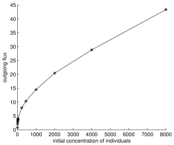
Figure 2: Outgoing flux for $T=5$ versus large initial data $M\to\infty$.

Figure 2 shows that there’s no apparent saturation for the outgoing flux with respect to the mass: the growth goes on in a polynomial fashion. The linear behavior has been obtained by setting to zero the aggregation and degradation coefficients.

In Figure 3, we see that the influence of variable diffusion coefficients is marginal; since a lot of mass exchange is happening in terms of species $u_{1}$, setting all the other coefficients $d_{2},\ldots,d_{N}$ to be lower than $d_{1}=1$ (i.e. bigger groups move somewhat slower than individuals) does not affect the output too much. Probably, the effect of diffusion could be stronger as soon as the effective diffusion coefficients are allowed to degenerate with locally vanishing $u_{i}$; this is a situation that can be foreseen in a modified setting Guo et al. (1988).

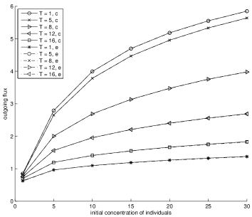
Figure 3: Homogeneous diffusion(c) and Stokes-Einstein diffusion(e). Note that the profiles are overlapping very closely.

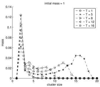
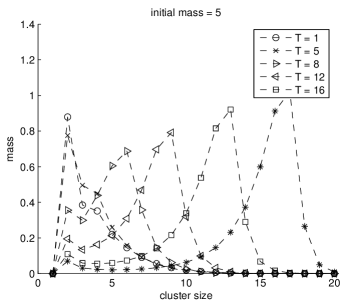
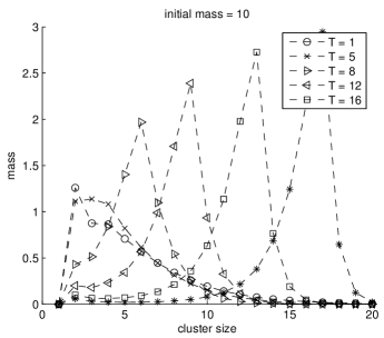
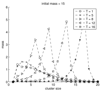
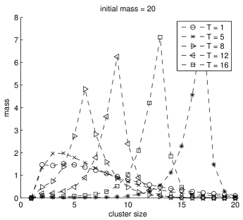
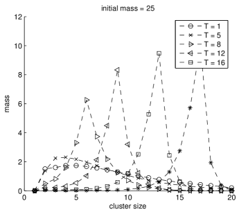
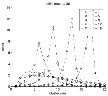
Figure 4: Steady-state mass distributions. Pile-up effect around group size $T$.

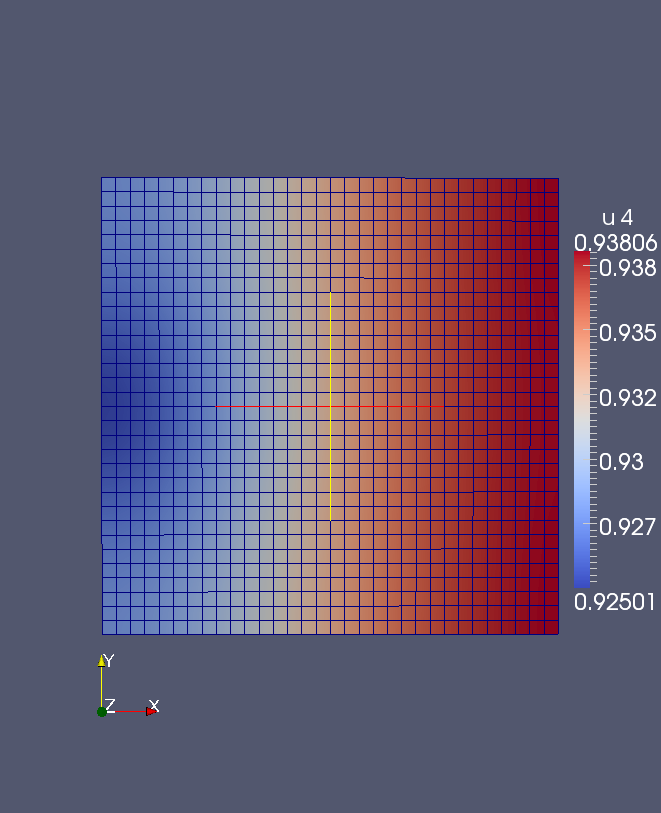
Figure 5: Clusters behavior close to the exit. The case of $u_{1}$–$u_{4}$.

In Figure 5, we see the mass escaping from the clusters $u_{1}$–$u_{4}$ in the neighborhood of the exit. Note the dramatic change in $u_{1}$ compared to what happens with the other group sizes. It is visible that large group have to stay in the queue until the small groups exit.

On the other hand, we can see in Figure 6 how the crowd breakage directly influences the outward flux. Essentially, a faster splitting of the groups tends to increase the averaged outgoing (evacuation) flux. This effect is due to our choice of boundary conditions at the exit.

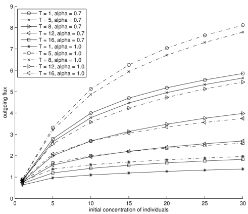
Figure 6: Comparison of outgoing flux for different values of degradation coefficients $\alpha$.

We mentioned in Section 2 that we expect that the way the threshold $T$ intervenes in the definition of the aggregation coefficients $\beta_{i}$ (compare (12)) essentially affects the maximum allowable group size. We can now see that close to the steady state situation, such situation happens. This effect is pointed out in Figure 4; the picture suggests that the mass of pedestrians piles-up in structures whose maximum lie around $T$.

Chapter 3 A lattice model for the reverse mosca cieca game

3 Microscopic dynamics

Using the lattice model presented in this section, we explore the effects of the microscopic non–exclusion on the overall exit flux (evacuation rate). More precisely, we look again at social thresholds and study this time the effect of the buddying threshold (of no–exclusion per site) on the dynamics of the crowd and investigate to which extent such approach confirms the following pattern revealed by investigations on real emergencies and also emphasized in Section 2: If the evacuees tend to cooperate and act altruistically, then their collective action tends to favor the occurrence of disasters.

Question (Q1) in Paragraph 1 drives any possible attempt of modeling pedestrians motion. In this section we show how an answer to this question can be setup by using a stochastic point of view.

Our reference scenario is here a microscopic one: Imagine to be one of the individuals in a dark (possibly crowded) corridor trying to save your life by quickly reaching one of the exits. You cannot see anything and, maybe, you do not have any a priori knowledge of the geometry of the corridor you have to exit from. It is not difficult to imagine that you will not be able to keep a constant direction of motion and that, in any case, it will be not chosen via some neat reasoning, but you will essentially chose it at random on the basis of what other people shout and scream. In some sense your motion will closely resemble that of the blinded kid playing mosca cieca with his friends.

Figure 7: The blind man’s buff game (the mosca cieca (ital.) game).

This simple remark triggered us to propose a stochastic model for the pedestrian motion in no–visibility areas based on a random walk scheme Cirillo and Muntean (2013, 2012). The random walk rule has been introduced by taking into account a possible interaction between the individuals, see the question (Q2) in Section 1.

Pedestrians move freely inside the corridor and like to buddy with people they accidentally meet at a certain point (site). The more people are localized at a certain site, the stronger the preference to attach to it. However if the number of people at a site reaches a threshold, then such site becomes not attracting for eventually new incomers.

Our lattice model provides a not so nice answer: In many situations, it seems much better not to cooperate. More precisely, in Section 4, we will see that simulations indicate to

• cooperate with one person at time;

• cooperate with more than one person only if the number of evacuees in the corridor is not too large.

Based on this idea we have announced in Cirillo and Muntean (2012) and then presented in details in Cirillo and Muntean (2013) a model for the motion of pedestrians governed by the following four mechanisms:

• in the core of the corridor, people move freely without constraints;

• the boundary is reflecting;

• people are attracted by bunches of other people up to a threshold (buddying mechanism);

• people are blind in the sense that there is no drift (desired velocity) leading them towards the exit.

Let $\Lambda\subset\mathbb{Z}^{2}$ be a finite square with odd side length $L$. We refer to this as the corridor. Each element $x$ of $\Lambda$ will be called a cell or site. The external boundary of the corridor is made of four segments made of $L$ cells each; the point at the center of one of these four sides is called exit. Let $N$ be positive integer denoting the (total) number of individuals inside the corridor $\Lambda$. We consider the state space $X:=\{0,\dots,N\}^{\Lambda}$. For any state $n\in X$, we let $n(x)$ be the number of individuals at cell $x$.

We define a Markov chain $n_{t}$ on the finite state space $X$ with discrete time $t=0,1,\dots$. The parameter of the process is the integer (possibly equal to zero) $T\geq 0$ called threshold. We finally define the function $S:\mathbb{N}\to\mathbb{N}$ such that

$$S(k):=\left\{\begin{array}[]{ll}1&\textrm{ if }k>T\\ k+1&\textrm{ if }k\leq T\\ \end{array}\right.$$

for any $k\in\mathbb{N}$. Note that for $k=0$ we have $S(0)=1$.

The transition matrix of the Markov chain is specified by assigning the stochastic rule according to which the individuals move on the lattice. At each time $t$, the $N$ individuals move simultaneously within the corridor according to the rules that will be specified in the following. These rules depend on the location of the pedestrian, we have to distinguish among four cases: bulk, corner, neighboring the wall, and neighboring the exit (see Figure 8. In the bulk: the probability for a pedestrian at the site $x$ to jump to one of the four neighboring sites $y_{1},\dots,y_{4}$ is

$$\frac{S(n(y))}{S(n(x))+S(n(y_{1}))+\cdots+S(n(y_{4}))}.$$

In a corner: the probability for a pedestrian at the site $x$ to jump to one of the two neighboring sites $y_{1}$ and $y_{2}$ is

$$\frac{S(n(y))}{S(n(x))+S(n(y_{1}))+S(n(y_{2}))}.$$

In a site close to the boundary: the probability for a pedestrian at the site $x$ to jump to one of the three neighboring sites $y_{1}$, $y_{2}$, and $y_{3}$ is

$$\frac{S(n(y))}{S(n(x))+S(n(y_{1}))+S(n(y_{2}))+S(n(y_{3}))}.$$

In front of the exit: the probability for a pedestrian at the site $x$ to jump to one of the three neighboring sites $y_{1}$, $y_{2}$, and $y_{3}$ in the bulk is

$$\frac{S(n(y))}{S(n(x))+S(n(y_{1}))+S(n(y_{2}))+S(n(y_{3}))+(T+1)},$$

whereas the probability to exit is

$$\frac{T+1}{S(n(x))+S(n(y_{1}))+S(n(y_{2}))+S(n(y_{3}))+(T+1)}.$$

In all the cases described above, the probability for the individual to stay at the same site $x$ (not to move) is $S(n(x))$ divided by the corresponding normalization denominator.

Figure 8: Schematic description of the different situation considered in the definition of the transition matrix.

The dynamics is then defined as follows: at each time $t$, the position of all the individuals on each cell is updated according to the probabilities defined above. If one of the individuals jumps on the exit cell a new individual is put on a cell of $\Lambda$ chosen randomly with the uniform probability $1/L^{2}$.

4 Playing games on lattices

The possible choices for the parameter $T$ correspond to two different physical situations. For $T=0$ the function $S(k)$ is equal to one whatever the occupation numbers. This means that each individual has the same probability to jump to one of its nearest neighbors or to stay on his site. This is the independent symmetric random walk case with not zero resting probability. The second physical case is $T>0$. For instance, $T=1$ means mild buddying, while $T=100$ would express an extreme buddying. No simple exclusion is included in this model: on each site one can cluster as many particles (pedestrians) as one wants. The basic role of the threshold is the following: The weight associated to the jump towards the site $x$ increases from $1$ to $1+T$ proportionally to the occupation number $n(x)$ until $n(x)=T$, after that level it drops back to $1$. Note that this rule is given on weights and not to probabilities. Therefore, if one has $T$ particles at $y$ and $T$ at each of its nearest neighbors, then at the very end one will have that the probability to stay or to jump to any of the nearest neighbors is the same. Differences in probability are seen only if one of the five (sitting in the core) sites involved in the jump (or some of them) has an occupation number large (but smaller than the threshold).

In Cirillo and Muntean (2013), we have studied numerically this model for $T=1,2,5,30$, and $100$. The Monte Carlo simulations have been all performed for $L=101$. For each value of the threshold we have studied the cases $N=100,600,1000,6000,10000$. For the choices $T=30$ and $T=100$ we have also analyzed the cases $N=2000,2200,2400,2600,2800,3000,3300$ and $N=1300,1600,2000,3000$, respectively.

The main quantity of interest that one has to compute is the average outgoing flux that is to say the ratio between the number of individuals which exited the corridor in the time interval $[0,t_{\textrm{f}}]$ and $t_{\textrm{f}}$. This quantity fluctuates in time, but for times large enough it approaches a constant value. In order to observe relative fluctuations smaller than $10^{-2}$ we had to use $t_{\textrm{f}}=5\times 10^{6}$. To capture the extreme buddying case $T=100$, we used $t_{\textrm{f}}=1.5\times 10^{7}$.

Figure 9: Averaged outgoing flux vs. number of pedestrians. The symbols $\circ$, $\times$, $*$, $\square$, and $+$ refer respectively to the cases $T=0,1,5,30,100$. The straight line has slope $8\times 10^{-6}$ and has been obtained by fitting the Monte Carlo data corresponding to the case $T=0$.

Figure 9 depicts our results, where the averaged outgoing flux is given as a function of the number of individuals. At $T=0$, that is when no buddying between the individuals is put into the model, the outgoing flux results proportional to the number of pedestrians in the corridor; indeed the data represented by the symbol $\circ$ in Figure 9 have been perfectly fitted by a straight line.

The appearance of the straight line was expected in the case $T=0$ since in this case the dynamics reduces to that of a simple symmetric random walk with reflecting boundary conditions; see also the straight line in Figure 1 (where we suspect that, microscopically, something very similar microscopically happens). This effect was studied rigorously in the one–dimensional case and via Monte Carlo simulations in dimension two in Andreucci et al. (2011). The order of magnitude of the slope can be guessed with a simple argument Andreucci et al. (2012): the typical time needed by the walker, started at random in the lattice, to reach the site facing the exit is of order of

$$\Big{(}\frac{1}{6}L\Big{)}^{2}\times 4L=\frac{1}{9}L^{3}.$$

The first term is the square of the average distance of a point inside a square of side length $L$ from the boundary of the square itself and the second one is the number of times the walker has to visit the internal boundary before facing the exit. Hence

$$\textrm{outgoing flux}=\frac{1}{t_{\textrm{f}}}N\frac{t_{\textrm{f}}}{L^{3}/9}=\frac{9}{L^{3}}\,N=8.73\times 10^{-6}\,N.$$

When a weak buddying effect is introduced in the model, that is in the case $T=1$, we find that if the number of individuals is small enough, say $N\leq 6000$, the behavior is similar to the one measured in the absence of buddying ($T=0$). At $N=10000$, on the other hand, we measure a larger flux; meaning that in the crowded regime small buddying favors the evacuation of the corridor [i.e. it favors the finding of the door].

The picture changes completely when buddying is increased. To this end, see the cases $T=5,30,100$. The outgoing flux is slightly favored when the number of individuals is low and strongly depressed when it this becomes high. The value of $N$ at which this behavior changes strongly depends on the threshold parameter $T$.

The question remains:

Why does the disaster occur at large threshold and large density?

It is not straightforward to understand how the model behaves in this regime. Inspired by theory behind particles percolation in porous media, one possible natural explanation would be that individuals cluster in bunches and that the resulting dynamics is characterized by the motion of these huge groups. At the moment we do not know if this explanation is the right one. In order to support it at least partially, we have computed the histogram of the size of the bunch at the center of the corridor; see Figure 10. Here we compare the cases $T=0$ and $T=100$ for $N=10000$ individuals. The histogram has been constructed by running a $10^{6}$ long simulation. The picture does suggest that the bunch formation is negligible in the former case while in the latter it is a possible mechanism.

Figure 10: Histogram of the size of the bunch of people occupying the center of the lattice for $N=10000$, $T=0$ (left), and $T=100$ (right).

Now, we can summarize our conclusions based on this microscopic model. Through a novel lattice model we have examined the effect of buddying mechanisms on the efficiency of evacuation in a smoky corridor (no–visibility area). With respect to the outgoing flux measured in absence of group formation, our model predicts that

• the existence of many small groups (threshold $T$ equal to one) favors the exit efficiency (compare points and straight line in figure 9: straight line is essentially the not–buddying case);

• strong gregariousness favors the exit efficiency only if the number of evacuees is small enough;

• the larger the threshold, the more dramatic is this effect.

In Heliavaara et al. (2012), the authors present an experiment whose purpose was to study evacuees exit selection under different behavioral objectives. The evacuation (egress) time of the whole crowd turned out to be shorter when the evacuees behave egoistically instead of behaving cooperatively. This is rather intriguing and counter intuitive fact, and it is very much in the spirit of the effect of the threshold $T$ we observed above.

Note that for low densities the buddying mechanism increases the outgoing flux, whereas at large densities the scenario is dramatic: isolated individuals may turn to have a bigger escape chance than a large group around a leader [behavior recommended by standard manuals on evacuation strategies, see e.g. NIB (2009), p. 122.]. This suggests that evacuation strategies should not rely too much only on the presence of a leader; see Katsikopoulos and King (2010) for a related scenario.

Chapter 4 Open issues

This research opens a series of fundamental questions. Some of them connect to the psychology of pedestrian groups that are essentially driven by features, behaviors, and not necessarily by desired velocities encoding the information on the location and accessibility of the exits. Some other questions are more general and refer to effect of the threshold on the general behavior of solutions to both cellular-like automata (lattice systems) as well as on Becker-Döring-like systems of differential equations (continuum systems).

We conclude the paper by enumerating a few detailed questions as well as less crystalized but promising links to other fields of science:

1. Is there a direct link between the models (or variants on the same theme) presented in Section 2 and in Section 3? Can one derive in the many-particle limit (i.e. $N\to\infty$)) Becker-Döring-like equations having as departure point a particle system with threshold dynamics governing the interactions? We expect that a few hints can be taken over from Großkinsky et al. (2005) at least in what the moderately stochastically interacting particle limit case is concerned. Note that some ideas on how one could possibly treat simple interacting-particle systems with threshold are also anticipated in Bodineau et al. (2010), e.g., in the context of modeling batteries. For the passage from the Becker-Döring-like system to the corresponding continuity equation, ideas from Niethammer (2004) may turn to be useful.

2. We do not know yet how pedestrians should behave if they don’t posses any information on the location of the exit. Difficult questions are: What is the right type of behavior in the dark? or How do people behave close to walls? To choose what is the best strategy for moving [e.g. cooperation (grouping, buddying, etc.) versus selfishness (walking away from groups)] one may also wish to explore basic aspects of the dynamics of non-momentum conserving inelastic collisions. Billiard dynamics, or biased billiards like those modeling the prisoner’s dilemma, or broader contexts involving stochastic game theory (see Szilagyi (2003)), perhaps involving non-standard (strongly non-Gaussian) scenarios, where energy can be exchanged between particles in a non-standard way need to be studied Eggels (2013). Recall that the Newtonian principle of action and reaction is not necessarily true anymore in this framework; see Haret (1910).

3. A quite similar pile-up effect to the one seen in Figure 4 appears as a result of the motion of edge dislocations on slip planes in steel plasticity. The dislocations are repulsively interacting defects naturally arising in the crystalline structure of materials (here dual phase steels). Their motion is typically accelerated by the action of a macroscopic stress. As result of this, the dislocations are pushed towards a piling-up in the boundary later present at the interface between the strong and weak material phase; see Geers et al. (2013); van Meurs et al. (2013) for mathematical evidence on the formation of the pile-up starting off from a suitably interacting particle system. Is there a hidden threshold mechanism responsible for the formation of the pile-up of dislocations? We suspect that the high contrast between the stiffnesses of the two steel phases is the responsible threshold. We plan to use a rigorous upscaling/homogenization procedure to shed more light on connecting density thresholds (high-contrast) with pilling-ups.

4. To which extent cooperation is profitable? is a basic question studied recently for instance in Curşeu et al. (2013).psychologists and socio- econo- physicists. neglecting the effect of population size, thresholds and boundary conditions, The authors of Curşeu et al. (2013) are pointing out the superiority of collaborative interaction rules as compared to follow-the-leader type of interactions, making clear connections between concepts like group rationality and deliberative democracy. From yet a different perspective, this subject is intimately connected to the dynamics of opinions (cf. e.g. the work by S. Galam; to get a hint on this see Galam (2011); Martins and Galam (2012) and references cited therein) as indicated also in Moshman (March 13, 2013) (in the spirit that deliberative democracy outreasons enlightened dictatorship). One could stretch more this idea towards eventual links to percolation theory applied this time not to a porous media setting, but rather to dynamically evolving networks (societies). We refer the reader to van Santen et al. (2010), for some preliminary thoughts around the idea of percolation thresholds occurring in structured social systems.

5. Both the lattice system and the population balances approach à la Becker-Döring share many similarities. However, there are a few essential differences between the two approaches. An important one is the following: For small $N$, the presence of the threshold $T$ seems to be beneficial for the particles leaving the lattice system; however this effect is lost completely in the Becker-Döring approach (compare Figure 5). This seems to be due to the choice of boundary conditions in the continuum system. On the other hand, we conjecture that the continuum limit of the lattice system is a sort of non-linear diffusion equation with inherited threshold, while we see that the Becker-Döring system is not emphasizing the threshold effects when changing the size (or nonlinearity) of the effective diffusion coefficient (see e.g. Figure 3). The challenging question is here: Derive (and then prove rigorously) the mean-field limit for the lattice system. Alternatively, one can reformulate the lattice model in terms of myopic random walkers in an exclusion process in the spirit of Landman and Fernando (2011) and then prove rigorously the validity of the corresponding mean-field model (a porous media-like equation).

6. Based on our working experience with continuum models with distributed microstructures, we expect that it is possible to couple the two models for groups dynamic within a single multiscale framework. The challenge here is to establish the right micro-macro transmission condition (in this case, a discrete-to-continuum coupling). We believe that steps in this direction are possible, inspired for instance by the way the human language is treated in Mitchener (2010) as a hybrid system.

Chapter 5 Becker-Döring system in the context of a two-scale modeling approach

5.A Background

This section contains a brief derivation of a structured-population model, which is a special case of a multi-feature continuity equation cf. Böhm (2012). It provides  a general framework for some of the equations we are dealing with. For a related derivation using densities, see Perthame (2007), e.g. At a more general scale the following considerations yield some sort of a transport equation or continuity equation, respectively, with two features being involved in the transport (also: cf. Smoluchowski (1917); Diekmann et al. (1998) et al.). In the present situation, the "location in the corridor" and the "group size" constitute the two "features". The first is a continuous, the second a discrete variable. Our aim is to derive a population-balance equation, (21), able to describe the evolution of pedestrian groups in obscured regions.

Fix $N\in\mathbb{N}$, let $\Omega\subset\mathbb{R}^{2}$ be the dark corridor (open, bounded with Lipschitz boundary), $S$ - the observation time interval and $K_{d}:=\left\{0,1,2,3,..,N\right\}$ - the collection of all admissible group sizes. We say that a $Y$ belongs to $K^{\prime}\subseteq K,$ if it belongs is part of some group with a size  K. Furthermore, $\mathfrak{A}_{\Omega}:=\mathfrak{B}^{2}(\Omega)$, $\mathfrak{A}_{S}:=\mathfrak{B}^{1}(S)$ are the corresponding Borel $\sigma$-algebras with the corresponding Lebesgue-Borel measures $\lambda_{x}:=\lambda^{2}$ and $\lambda_{t}:=\lambda^{1},$ respectively; $\mathfrak{A}_{K_{d}}:=\mathfrak{p}(K_{d})$ is equipped with the counting measure $\lambda_{c}^{\prime}(K):=\left|K^{\prime}\right|$. We call $\lambda_{tx}:=\lambda_{t}\otimes\lambda_{x}$ the space-time measure and set $\lambda_{txc}:=\lambda_{t}\otimes\lambda_{x}\otimes\lambda_{c_{j}},$ $\mathfrak{A}_{\Omega K_{d}}:=\mathfrak{A}_{\Omega}\otimes\mathfrak{A}_{K_{d}},$ $\mathfrak{A}_{S\Omega K_{d}}:=\mathfrak{A}_{S}\otimes\mathfrak{A}_{\Omega}\otimes\mathfrak{A}_{K_{d}}.$

5.B Derivation of the model

Fix $t\in S,$ let $\Omega^{\prime}\in\mathfrak{A}_{\Omega},$ $K^{\prime}\in\mathfrak{A}_{K_{d}},$ $S^{\prime}\in\mathfrak{A}_{S}$, introduce

$$\begin{array}[c]{c}\mu_{Y}(t,\Omega^{\prime}\times K^{\prime}):=\text{ number of }Y^{\prime}s\text{ present in }\Omega^{\prime}\text{ }\\ \text{at time }t\text{ and belonging to the group }K^{\prime}\\ \end{array}$$ (13)

and two production quantities

$$\begin{array}[c]{c}\mu_{PY\pm}(S^{\prime}\times\Omega^{\prime}\times K^{\prime}):=\text{ number of }Y^{\prime}s\text{ which are added }\\ \text{to (subtracted from) }\Omega^{\prime}\times K^{\prime}\text{ during }S^{\prime}\text{ and}\\ \mu_{PY}=\mu_{PY+}-\mu_{PY-}.\end{array}$$ (14)

Note that these numbers might be non-integer.

Given the nature of the problems we are dealing with, we postulate - as a part of the modeling-

(P1)   For all $K^{\prime}\in$ $\mathfrak{A}_{K_{d}},$ $\Omega^{\prime}\in$ $\mathfrak{A}_{\Omega}$   and $t\in S:\mu_{Y}(t,\cdot\times K^{\prime})$ and $\mu_{Y}(t,\Omega^{\prime}\times\cdot)$ are measures on their respective $\sigma$-algebras $\mathfrak{A}_{\Omega}$ and $\mathfrak{A}_{K_{d}},$ respectively.

(P2) $\ \ \mu_{PY\pm}(S^{\prime}\times\Omega^{\prime}\times\cdot),$ $\mu_{PY\pm}(S^{\prime}\times\cdot\times K^{\prime})$ and $\mu_{PY\pm}(\cdot\times\Omega^{\prime}\times K^{\prime})$ are measures on their respective $\sigma$-algebras.

Now, we are in the position to formulate a

$$\begin{array}[c]{c}\text{Balance principle:}\\ \mu_{Y}(t+h,\Omega^{\prime}\times K^{\prime})-\mu_{Y}(t,\Omega^{\prime}\times K^{\prime})=\mu_{PY}(S^{\prime}\times\Omega^{\prime}\times K^{\prime})\\ \text{for all }t,t+h\in S,\text{ }\Omega^{\prime}\times K^{\prime}\in\mathfrak{A}_{\Omega}\times\mathfrak{A}_{K_{d}},\text{ }S^{\prime}:=(t,t+h].\\ \end{array}$$ (15)

Addition to $\Omega^{\prime}\times K^{\prime}$, modeled by $\mu_{PY+},$ can happen by addition inside of $\Omega^{\prime}\times K^{\prime}$ as well as by fluxes into $\Omega^{\prime}\times K^{\prime}.$ A similar remark applies to subtraction and $\mu_{PY-}$. This gives rise to assume $\mu_{PY+}$ to be the sum of an interior production part, $\mu_{PY+}^{int},$ and a flux part, $\mu_{PY+}^{flux}.$ We proceed similarly with $\mu_{PY-}$ and have, with the

$$\text{net productions }\mu_{PY}^{int}:=\mu_{PY+}^{int}-\mu_{PY-}^{int}\text{ and \ }\mu_{PY}^{flux}:=\mu_{PY+}^{flux}-\mu_{PY-}^{flux}:$$

$$\ \ \mu_{PY}=\mu_{PY}^{int}+\mu_{PY}^{flux}=\left(\mu_{PY+}^{int}-\mu_{PY-}^{int}\right)+\left(\mu_{PY+}^{flux}-\mu_{PY-}^{flux}\right).$$ (16)

We extend $\mu_{Y}(t,\cdot\times\cdot)$ and $\mu_{PY\pm}(\cdot\times\cdot\times\cdot)$ by the usual procedure to measures $\overline{\mu}_{Y}=\mu_{Y}(t,\cdot)$ and $\overline{\mu}_{PY\pm}=\overline{\mu}_{PY\pm}(\cdot)$ on the product algebras $\mathfrak{A}_{\Omega}\otimes\mathfrak{A}_{K_{d}}$ and $\mathfrak{A}_{S}\otimes\mathfrak{A}_{\Omega}\otimes\mathfrak{A}_{K_{d}},$ respectively.

Note that the quantities in (P1) and (P2) and the extensions are finite.

The following postulate prevents accumulation on sets of measure zero. It reads as

(P3)  $\overline{\mu}_{Y}(t,\cdot)\ll\lambda_{xc}$ (absolutely continuous).

Therefore, for all $t\in S$ there are integrable Radon-Nikodym densities $u(t,\cdot)=\frac{d\overline{\mu}_{Y}(t,\cdot)}{d\lambda_{xc}},$ i.e.

$$\overline{\mu}_{Y}(t,Q^{\prime})=\int_{Q^{\prime}}u(t,(x,i))d\lambda_{xc}\text{ \ for all }Q^{\prime}\in\mathfrak{A}_{\Omega K}.$$ (17)

The absolute-continuity assumption

(P4)  $\overline{\mu}_{PY}^{int}\ll\lambda_{txc}$

excludes the presence of $Y^{\prime}s$ on sets of $\lambda_{txc_{1}}$-measure zero. Moreover it assures the existence of the Radon-Nikodym density

$$f_{PY}^{int}:=\frac{d\overline{\mu}_{PY}}{d\lambda_{txc}}\in L_{loc}^{1}(S\times\Omega\times K_{d},\mathfrak{A}_{S\Omega K_{d}},\lambda_{txc}).$$ (18)

In order to get a reasonable idea for a representation of the flux measure we consider the special case $Q^{\prime}=\Omega^{\prime}\times K^{\prime}$ with, say, $K^{\prime}=\left\{a,a+1,...,b\right\}\in\mathfrak{p}(K_{d}).$ The "surface"

$$\mathfrak{F}:=\Omega^{\prime}\times\left\{a\right\}\cup\Omega^{\prime}\times\left\{b\right\}\cup\partial\Omega^{\prime}\times K^{\prime}$$

is the location of any interaction with the outside of $Q^{\prime}$. There are two locations on $\mathfrak{F}$ to enter or leave $Q^{\prime}$ from the outside - one via $\mathfrak{F}_{1}:=\Omega^{\prime}\times\left\{a\right\}\cup\Omega^{\prime}\times\left\{b\right\},$ the other one through $\mathfrak{F}_{2}:=\partial\Omega^{\prime}\times K^{\prime}$  (see Figure 11).

Figure 11: Special interactions regions on the surface $\mathfrak{F}$.

The unit-outward normal field $\mathbf{n}=\mathbf{n}(x,\kappa)$ on $\mathfrak{F}$ can be split into two orthogonal components, $\mathbf{n}=\mathbf{n}_{x}+\mathbf{n}_{\kappa},$ $\mathbf{n}_{x}=(n_{x},0),$ $\mathbf{n}_{\kappa}=(0,n_{\kappa}),$ respectively. It is $n_{\kappa}(x,a)=-1$, $n_{\kappa}(x,b)=+1$ and $n_{x}=n_{x}(x,\kappa)$ is the a.e. existing outward normal on $\partial\Omega.$ Borrowing from the theory of Cauchy interactions, cf. Schuricht (2007), e.g..

(P5) we assume for all $t\in S$ the existence of two vector fields

$$j_{x}(t,\cdot) : \Omega\times K_{d}\rightarrow\mathbb{R}^{2}$$

$$j_{\kappa} : \Omega\times K_{d}\rightarrow\mathbb{R}$$

with

$$\overline{\mu}_{PY}^{flux}:=\overline{\mu}_{PYx}^{flux}+\overline{\mu}_{PY\kappa}^{flux}\text{,}$$

where

$$\begin{array}[c]{rl}\text{ }\\ \overline{\mu}_{PYx}^{flux}(S^{\prime}\times\Omega^{\prime}\times K^{\prime})&:=\int_{S^{\prime}}\int_{\mathfrak{F}_{{}_{2}}}-j_{x}(\tau,x,i)\cdot n_{x}(x,i)d\sigma_{x}d\lambda_{c}d\tau\text{ \ }\\ &\text{and}\\ \overline{\mu}_{PY\kappa}^{flux}(S^{\prime}\times\Omega^{\prime}\times K^{\prime})&:=\int_{S^{\prime}}\int_{\Omega^{\prime}}-j_{\kappa}(\tau,x,b)n_{\kappa}(x,b)\\ &-j_{\kappa}(\tau,x,a)n_{\kappa}(x,a)dxd\tau.\\ \end{array}$$ (19)

In (19), $\sigma_{x}$ - is the $1D$-surface (= curve length-) measure. $\overline{\mu}_{PYx}^{flux}(S^{\prime}\times\Omega^{\prime}\times K^{\prime})$ calculates the net gain/loss of the $Y^{\prime}s$ in $\Omega^{\prime}$ belonging to one of the size groups from $K^{\prime}$ due to physical motion from/to the outside of $\Omega^{\prime}$ into/out of $\Omega^{\prime}$.

Furthermore, $\overline{\mu}_{PY\kappa}^{flux}(S^{\prime}\times\Omega^{\prime}\times\left\{i\right\})$ calculates the net gain/loss of the $Y^{\prime}s$ in $\Omega^{\prime}$ belonging to the size group labelled by $i$ due to reasons within $K$. Since, in the given situation of Section 2, there is no interaction with groups of size $\kappa>N$ or $\kappa<0$ (these group sizes are not admissible!), we have to require

$$j_{\kappa}(t,x,0)=j_{\kappa}(t,x,N)=0\text{ \ for all }t\in S,\text{ }x\in\Omega.$$ (20)

Introducing the discrete partial derivative by

$$\text{ }\partial_{i}^{d}j_{\kappa}(t,x,i):=j_{\kappa}(t,x,i+1)-j_{\kappa}(t,x,i),\text{ }i\in K$$

and assuming $u,$ $f_{PY}^{int},$ $\operatorname{div}_{x}j_{x}$ and $\partial_{\kappa}^{d}j_{\kappa}$ to be sufficiently regular, we obtain

$$\overline{\mu}_{PY}^{flux}(S^{\prime}\times Q^{\prime}) =\int_{S^{\prime}}\int_{Q^{\prime}}-\operatorname{div}_{x}(j_{x}(\tau,x,i)d\lambda_{c}dxd\tau$$

$$+\int_{S^{\prime}}\int_{Q^{\prime}}-\partial_{i}^{d}j_{\kappa}(t,x,i)d\tau dxd\lambda_{c}.$$

Combining (15) - (19), Fubini’s theorem, and division by $h$, imply

$$\begin{array}[c]{c}\int_{Q^{\prime}}\frac{1}{h}\left(u(t+h,x,i)-u(t,x,i)\right)dxd\kappa\\ =\int_{Q^{\prime}}\frac{1}{h}\int_{t}^{t+h}\left(f_{PY}^{int}(\tau,x,i)-\left(\operatorname{div}_{x}j_{x}(\tau,x,i)+\partial_{i}^{d}j_{\kappa}(t,x,i)\right)\right)d\tau dxd\lambda_{c}.\\ \end{array}$$

Under appropriate smoothness conditions on $u,$ $f_{PY}^{int},$ $j_{x}$ and $j_{\kappa\text{ \ }}$we obtain in the limit $h\rightarrow 0$ (the classical continuity equation with a slightly different interpretation of the entries)

$$\frac{\partial u}{\partial t}(t,x,i)+\left(\operatorname{div}_{x}j_{x}+\partial_{i}^{d}j_{\kappa}(t,x,i)\right)=f_{PY}^{int}(t,x,i).$$ (21)

5.C Connection with the model in Section 2:

In order to obtain a workable model, one has to specify the flux vectors $j_{x}$ and $j_{\kappa}$ as well as $f_{PY}^{int}.$ In Section 2 this has been done in (1) to (6) by setting

$i=1,...,N$ (there) = $i=1,...,N$ (here), $u_{i}(t,x)$ (there) $=$ $u(t,x,i)$ (here), $-D_{i}\nabla_{x}u_{i}(t,x)$ (there) =$\ j_{x}(t,x,i)\$(here),

$$f_{PY}^{int}(t,x,i)\mbox{(here)}=\left\{\begin{array}[]{lr}\sum\nolimits_{i=1}^{N}\alpha_{i}u_{i}-\sum\nolimits_{i=1}^{N}+\beta_{i}u_{i}u_{1}&\mbox{ if }i=1,\\ \beta_{i-1}u_{i-1}u_{1}-\beta_{i}u_{i}u_{1}&\mbox{ if }i\in\{2,...,N-1\},\\ \beta_{N}u_{N-1}u_{1}&\mbox{ if }i=N,\\ \end{array}\right.$$

respectively.

The discrete derivative $j_{\kappa}(t,x,i)$ (here) corresponds to

$$j_{\kappa}(t,x,i) = -\alpha_{i}u_{i}(t,x),\ i=1,2,...,N-1,$$

$$j_{\kappa}(t,x,0) = j_{\kappa}(t,x,N)=0.$$

5.D Derivation of the model in Section 2:

Specifying $j_{x}(t,x,i)$ as some sort of a diffusion flux in the manner above means: Individual groups of size $i$ recognize whether a group of the same size is in their immediate neighborhood and they tend to avoid moving into the direction of such groups. Employing a Fickian law seems to be the simplest way to model this. $f_{PY}^{int}$ models interactions (= merging)  between groups of size $i\in K$ and "groups" of size $i=1$: If a single (i.e. a group of size one) hits a group of size $i<N$, then it might happen, that this single merges with the group. This turns the group into a group of size $i+1$ and leads to a "gain" for groups of size $i+1$ (modeled by $+\beta_{i}u_{i}u_{1}$) and a loss for groups of size $i$ (modeled by $-\beta_{i}u_{i}u_{1}$). In any such joining situation the group with $i=1$ looses members (modeled by $-{\textstyle\sum\nolimits_{i=2}^{N}}\beta_{i}u_{i}u_{1}$). Note, that this model allows only for direct interaction between groups of size $i$ with groups of size $1$! The $\alpha$-terms model some "degradation" effect: It might happen, that an individual leaves a group of size $i\geq 2$. This leads to a loss for the groups of size $i$ (modeled by $-\alpha_{i}u_{i}$), a gain for the groups of size $i-1$ and a gain for the groups with $i=1$ (modeled by ${\textstyle\sum\nolimits_{i=2}^{N}}\alpha_{i}u_{i}$). $\alpha_{i},$ $\beta_{i}\geq 0$ and $D_{i}>0$ are empirical and assumed to be constant.

Note: In the abstract approach the degradation terms express a flux rather than a volume source or sink. In the same way as aging can be seen as a flux ("people change their age group by aging with (speed 1)" ) $Y$’s change their size group by "degradation" of their group. Nevertheless: For fixed $i$, the expressions $\alpha_{i}u_{i}$ and $\alpha_{i-1}u_{i-1}$ still remain "volume sources" and "sinks", respectively. It’s just two different ways to look at the same thing.

References

- NIB (2009) Basisopleiding Bedrijfshulpverlener. NIBHV – Nederlands Instituut voor Bedrijfshulpverlening, Rotterdam, 2009.
- Andreucci et al. (2011) D. Andreucci, D. Bellaveglia, E. N. M. Cirillo, and S. Marconi. Monte Carlo study of gating and selection in potassium channels. Phys. Rev. E, 84:021920, 2011.
- Andreucci et al. (2012) D. Andreucci, D. Bellaveglia, E. N. M. Cirillo, and S. Marconi. Effect of intracellular diffusion on current–voltage curves in potassium channels. arXiv: 1206.3148, 2012.
- Bodineau et al. (2010) T. Bodineau, B. Derrida, and J. L. Lebowitz. A diffusive system driven by a battery or by a smoothly varying field. Journal of Statistical Physics, 140(4):648–675, 2010.
- Böhm (2012) M. Böhm. Lecture Notes in Mathematical Modeling. Universität Bremen, Germany, 2012. Fachbereich Mathematik und Informatik,.
- Chepizhko et al. (2013) O. Chepizhko, E. Altmann, and F. Peruani. Collective motion in heterogeneous media. Phys. Rev. Lett., 2013:to appear, 2013.
- Cirillo and Muntean (2013) E. N. M. Cirillo and A. Muntean. Dynamics of pedestrians in regions with no visibility – a lattice model without exclusion. Physica A: Statistical Mechanics and its Applications, 392(17):3578 – 3588, 2013.
- Cirillo and Muntean (2012) E. N. M. Cirillo and A. Muntean. Can cooperation slow down emergency evacuations? Comptes Rendus Mecanique, 340:626–628, 2012.
- Curşeu (2009) P. L. Curşeu. Group dynamics and effectiveness: A primer. In S. Boros, editor, Organizational Dynamics, chapter 7, pages 225–246. Sage, London, 2009.
- Curşeu et al. (2013) P. L. Curşeu, R. J. Jansen, and M. M. H. Chappin. Decision rules and group rationality: Cognitive gain or standstill? PLoS ONE, 8(2):e56454, 2013.
- Diekmann et al. (1998) O. Diekmann, M. Gyllenberg, J. A. J. Metz, and H. R. Thieme. On the formulation and analysis of general deterministic structured population models I. Linear theory. Journal of Mathematical Biology, 36(4):349–388, 1998.
- Dyer et al. (2009) J. R. G. Dyer, A. Johansson, D. Helbing, I. D. Couzin, and J. Krause. Leadership, consensus decision making and collective behaviour in humans. Philosophical Transactions of the Royal Society: Biological Sciences, 364:781–789, 2009.
- Edward (1970) J. T. Edward. Molecular volumes and the Stokes-Einstein equation. Journal of Chemical Education, 47(4):261, 1970.
- Eggels (2013) A. Eggels. Social billiards – a novel approach to crowd dynamics in dark (Bachelor thesis, TU Eindhoven), 2013.
- Evers and Muntean (2011) J. H. M. Evers and A. Muntean. Modeling micro-macro pedestrian counterflow in heterogeneous domains. Nonlinear Phenomena in Complex Systems, 14(1):27–37, 2011.
- Fang et al. (2012) Z.-M. Fang, W.-G. Song, J. Zhang, and H. Wu. A multi-grid model for evacuation coupling with the effects of fire products. Fire Technology, 48:91–104, 2012.
- Galam (2011) S. Galam. Collective beliefs versus individual inflexibility: The unavoidable biases of a public debate. Physica A-Statistical Mechanics and Its Applications, 390:3036–3054, 2011.
- Geers et al. (2013) M.G.D. Geers, R.H.J. Peerlings, M.A. Peletier, and L. Scardia. Asymptotic behaviour of a pile-up of infinite walls of edge dislocations. Arch. Ration. Mech. Analysis, 209(2):495–539, 2013.
- Großkinsky et al. (2005) S. Großkinsky, C. Klingenberg, and K. Ölschläger. A rigorous derivation of Smoluchowski’s equation in the moderate limit. Stochastic Analysis and Applications, 22(1):113–141, 2005.
- Guo et al. (1988) M. Z. Guo, G. C. Papanicolaou, and S. R. S. Varadhan. Nonlinear diffusion limit for a system with nearest neighbor interactions. Comm. Math. Phys., 118(1):31–59, 1988.
- Guo et al. (2012) X. Guo, J. Chen, Y. Zheng, and J. Wei. A heterogeneous lattice gas model for simulating pedestrian evacuation. Physica A: Statistical Mechanics and its Applications, 391(3):582 – 592, 2012.
- Haret (1910) S. Haret. Mécanique sociale. Gauthier-Villars, Paris, 1910.
- Helbing and Molnar (1995) D. Helbing and P. Molnar. Social force model for pedestrian dynamics. Physical Review E, 51(5):4282–4286, 1995.
- Heliavaara et al. (2012) S. Heliavaara, J.-.I. Kuusinen, T. Rinne, T. Korhonen, and H. Ehtamo. Pedestrian behavior and exit selection in evacuation of a corridor: An experimental study. Safety Science, 50(2):221 – 227, 2012.
- Jin (1978) T. Jin. Visibility through fire smoke. Journal of Fire and Flammability, 9:135–155, 1978.
- Jin and Yamada (1985) T. Jin and T. Yamada. Irritating effects of fire on visibility. Fire Science and Technology, 5:79–90, 1985.
- Katsikopoulos and King (2010) K. V. Katsikopoulos and A. J. King. Swarm intelligence in animal groups: When can a collective out-perform an expert? PLOS One, 5:11, 2010.
- Kirchner and Schadschneider (2002) A. Kirchner and A. Schadschneider. Simulation of evacuation processes using a bionics-inspired cellular automaton model for pedestrian dynamics. Physica A: Statistical Mechanics and its Applications, 312(1-2):260 – 276, 2002.
- Kobes et al. (2010) M. Kobes, I. Helsloot, B. de Vries, and J. G. Post. Building safety and human behaviour in fire: A literature review. Fire Safety Journal, 45(1):1 – 11, 2010.
- Krehel et al. (2012) O. Krehel, A. Muntean, and P. Knabner. On modeling and simulation of flocculation in porous media. In A.J. Valochi (Ed.), Proceedings of XIX International Conference on Water Resources. (pp. 1-8) CMWR, University of Illinois at Urbana-Champaign, 2012.
- Landman and Fernando (2011) K. A. Landman and A. E. Fernando. Myopic random walkers and exclusion processes: Single and multispecies. Physica A: Statistical Mechanics and its Applications, 390:3742 – 3753, 2011.
- Le Bon (2008) G. Le Bon. La psychologie des foules. The Echo Library, Middlesex, 2008.
- Manzoni (1909) A. Manzoni. I Promessi Sposi (The betrothed). P. F. Collier and Son Comp., New York, 1909.
- Martins and Galam (2012) A. C. R. Martins and S. Galam. The building up of individual inflexibility in opinion dynamics. CoRR, abs/1208.3290, 2012.
- Mitchener (2010) W. Mitchener. Mean-field and measure-valued differential equation models for language variation and change in a spatially distributed population. SIAM J. Math. Anal., 42(5):1899–1933, 2010.
- Moshman (March 13, 2013) D. Moshman. Deliberative democracy outreasons enlightened dictatorship. Politics section, Huffington post, March 13, 2013.
- Muşatescu (1978) V. Muşatescu. Extravagantul Conan Doi: De-a v-aţi ascunselea. De-a baba oarba. Cartea Românească, 1978.
- Niethammer (2004) B. Niethammer. Macroscopic limits of the Becker-Doring equations. Commun. Math. Sci., 2(1):85 – 92, 2004.
- Perthame (2007) B. Perthame. Transport Equations in Biology. Frontiers in Mathematics. Birkhauser, Basel, Boston, Berlin, 2007.
- Piccoli and Tosin (2011) B. Piccoli and A. Tosin. Time-evolving measures and macroscopic modeling of pedestrian flow. Arch. Ration. Mech. Anal., 199(3):707–738, 2011.
- Portuondo y Barceló (1912) A. Portuondo y Barceló. Apuntes sobre Mecánica Social. Establecimiento Topográfico Editorial, Madrid, 1912.
- Presutti (2013) E. Presutti. Personal communication, 2013.
- Ray et al. (2012) N. Ray, A. Muntean, and P. Knabner. Rigorous homogenization of a Stokes- Nernst-Planck-Poisson system. Journal of Mathematical Analysis and Applications, 390(1):374 – 393, 2012.
- Schadschneider et al. (2009) A. Schadschneider, W. Klingsch, H. Kluepfel, T. Kretz, C. Rogsch, and A. Seyfried. Evacuation dynamics: Empirical results, modeling and applications. In R. A. Meyers, editor, Encyclopedia of Complexity and System Science, volume 3, pages 31–42. Springer Verlag, Berlin, 2009.
- Schadschneider et al. (2011) A. Schadschneider, D. Chowdhury, and K. Nishinari. Stochastic Transport in Complex Systems. Elsevier, 2011.
- Schuricht (2007) F. Schuricht. A new mathematical foundation for contact interactions in continuum physics. Arch. Ration. Mech. Anal., 1984:169–196, 2007.
- Smoluchowski (1917) M. Smoluchowski. Versuch einer mathematischen Theorie der Koagulationskinetik kolloider Lösungen. Z. Phys. Chem., 92:129–168, 1917.
- Suma et al. (2012) Y. Suma, D. Yanagisawa, and K. Nishinari. Anticipation effect in pedestrian dynamics: Modeling and experiments. Physica A: Statistical Mechanics and its Applications, 391:248 – 263, 2012.
- Szilagyi (2003) M. N. Szilagyi. Simulation of multi-agent Prisoners’ Dilemmas. Syst. Anal. Model. Simul., 43(6):829–846, June 2003.
- Topaz and Bertozzi (2004) C. M. Topaz and A. L. Bertozzi. Swarming patterns in a two-dimensional kinematic model for biological groups. SIAM J. Appl. Math., 65:152–174, 2004.
- van Meurs et al. (2013) P. van Meurs, A. Muntean, and M. A. Peletier. Upscaling of dislocations walls in finite domains. unpublished, Eindhoven University of Technology, 2013.
- van Santen et al. (2010) R. van Santen, D. Khoe, and B. Vermeer. 2030: Technology That Will Change the World. Oxford University Press, UK, 2010.
- Zheng et al. (2011) Y. Zheng, B. Jia, X.-G. Li, and N. Zhu. Evacuation dynamics with fire spreading based on cellular automaton. Physica A: Statistical Mechanics and its Applications, 390:3147–3156, 2011.
- Богданов (2001) К. Богданов. Игра в жмурки: сюжет, контекст, метафора. Искусство-СПБ, 2001.