Growing discharge trees with self-consistent charge transport: the collective dynamics of streamers

Abstract

We introduce the generic structure of a growth model for branched discharge trees that consistently combines a finite channel conductivity with the physical law of charge conservation. It is applicable, e.g., to streamer coronas near tip or wire electrodes and ahead of lightning leaders, to leaders themselves and to the complex breakdown structures of sprite discharges high above thunderclouds. Then we implement and solve the simplest model for positive streamers in ambient air with self-consistent charge transport. We demonstrate that charge conservation contradicts the common assumption of dielectric breakdown models that the electric fields inside all streamers are equal to the so-called stability field and we even find cases of local field inversion. We also discuss the charge distribution inside discharge trees, which provides a natural explanation for the observed reconnections of streamers in laboratory experiments and in sprites. Our simulations show the structure of an overall “streamer of streamers” that we name collective streamer front, and predict effective streamer branching angles, the charge structure within streamer trees, and streamer reconnection.

I Introduction

I.1 Phenomena and state of understanding

When a high electric voltage is suddenly applied to ionizable matter, electric breakdown frequently takes the form of growing filaments, and these filaments can form a complex tree structure. Discharge trees are observed in streamer coronas around tip or wire electrodes, in the streamer coronas ahead of propagating lightning leaders Rakov and Uman (2003) and in the (hot) leaders themselves. Streamer discharge trees also appear in transient luminous events such as jets Wescott et al. (1995), gigantic jets Su et al. (2003) and sprites Franz et al. (1990) between thunderclouds and the ionosphere. Streamer and leader trees are a generic response to high voltage pulses; they appear in various gases, liquids and solids in plasma and high voltage technology.

Our understanding of such non-thermal, filamentary electrical discharges is remarkably unbalanced. On the one hand, we are now reaching a very detailed knowledge on their microphysics; this includes models of electron energy distributions Li et al. (2012a), and of transport coefficients and cross-sections of the main reactions, at least for air and other common gas compositions. This knowledge translates into sophisticated and reasonably accurate models of single streamers Eichwald et al. (2008); Pancheshnyi et al. (2005); Qin et al. (2012); Liu (2010); Luque and Ebert (2012); Li et al. (2012b), the initiation of streamer branching Li et al. (2012a); Luque and Ebert (2011); Li et al. (2012b) and the merging of two nearby streamers Luque et al. (2008a); Bonaventura et al. (2012). On the other hand, we barely understand most macroscopic processes in a fully developed corona or streamer tree involving hundreds or thousands of mutually interacting plasma filaments. The large scale transport of charge, the internal electric fields and the influence of the many surrounding streamers on one single streamer are rarely discussed in the literature. However, these mechanisms are relevant for the propagation of long sparks Raizer (1991); Bondiou and Gallimberti (1994); Kochkin et al. (2012) and the approach of lightning leaders towards protecting rods. The overall tree structure also determines which volume fraction of the medium is “treated” by the discharge, creating radicals, ions and subsequent chemical products relevant for plasma technology and for the production of greenhouse gases during a thunderstorm.

Most studies on the growth of electrical discharge trees descend from the Dielectric Breakdown Model (DBM) Niemeyer et al. (1984) that Niemeyer et al. proposed in 1984 to explain the fractal properties of some electrical discharges such as Lichtenberg figures that propagate over a dielectric surface. In their model, a discharge tree expands in discrete time-steps by the stochastic addition of new segments with a probability that depends on the local electric field.

We are not aware of many models of fully three-dimensional streamer trees not based on the DBM. Only Akyuz et al. Akyuz et al. (2003) modeled streamers as a tree of connected, perfectly conducting cylinders that propagate according to simple rules based on the value of the electric field surrounding the tips. The computations required to solve the electrostatic problem limited their simulations to small trees with less than 10 branches.

The original DBM as well as Akyuz et al. (2003) assume that the channels in the tree are perfectly conducting, but there is strong experimental evidence that the electric potential decreases along a discharge channel.

I.2 Electric fields inside discharge trees: stability field versus self-consistent charge transport

The common approach to introduce a potential decay along a streamer channel and inside the streamer corona is to assume that the electric field inside a streamer has a fixed value, the so-called stability field. E.g., in air at standard temperature and pressure the stability field of positive streamers is thought to be 4 to 5 kV/cm. A fixed stability field is used to model the streamer corona that precedes a leader in a long spark discharge Goelian et al. (1997); Becerra and Cooray (2006); Arevalo and Cooray (2011) or the enormous streamer trees in sprite discharges high above thunderstorms Pasko et al. (2000).

However, the concept of a fixed field inside streamer channels lacks any theoretical support. Rather, it is based on a phenomenological interpretation of experiments that nevertheless have not measured the internal streamer fields. Originally, the concept of stability field refered to the minimum average applied field for sustained streamer propagation in a gap between parallel electrodes Allen and Ghaffar (1995). The existence of such a minimum field around 4 to 5 kV/cm was interpreted Gallimberti (1972, 1979) in terms of a now discarded model of streamers as isolated patches of charge. Later it was found that the relation between the applied potential at the originating electrode $U$ and the longest streamer length $L$ is roughly linear with $U/L\approx(4.5-5)\,\mathrm{kV/cm}$ in air Bazelyan and Raizer (2010). Since this value was close to the existing concept of an stability field, the results were interpreted as indicating that the stability field was the electric field inside the streamer channel. However, even the earliest numerical simulations of 2d streamers Dhali and Williams (1987) already showed a clearly non-constant electric field in the channel. As we will see, this variation is enhanced by the collective dynamics of a streamer tree. Indeed, our results will show that the assumption of a constant electric field in all streamers is in contradiction with a consistent charge transport model, as long as conductivity stays finite.

Recent simulations of density models resolving the inner structure of streamers already have established the relevance of a self-consistent charge transport model for the dynamics of streamer channels, and, in particular, for the dynamics of the electric field in the channel. For upper-atmospheric streamers, Liu Liu (2010) and Luque and Ebert Luque and Ebert (2010) independently showed that the re-brightening of sprite streamer trails is due to a second wave associated with a significant increase of the electric field in the sprite channel; Luque and Gordillo-Vázquez Luque and Gordillo-Vázquez (2011) postulated later that sprite beads are also caused by persisting and localized electric fields. These electric fields may only persist due to a finite conductivity in the streamer channel Gordillo-Vázquez and Luque (2010), which also sets their decay times.

To our knowledge, the only DBM-inspired models that treat the charge transport self-consistently appear in the context of discharge trees in dielectrics Noskov et al. (2001), generated when a solid insulator is subjected to an intense, repetitive electrical stress Dissado and Sweeney (1993).

I.3 Content of the paper

In the present paper we first outline the general structure of a model for growing discharge trees that consistently incorporates charge conservation. Then we introduce the simplest model for a streamer corona as a tree structure of linear channel segments with a finite fixed diameter and with a finite fixed conductivity. The streamer channel tips advance and branch according to simple, phenomenologically motivated rules. We analyze the internal electric fields and the transport of charge in fully branched, extensive streamer coronas. This is a stepping stone towards more realistic and detailed models and, although many improvements of our approach are straightforward, we have often kept complexity at a minimum in order to focus on the overall qualitative behavior of streamer trees with realistic conductivities and consistent charge transport, which appears to be largely unexplored in the existing literature.

The paper is organized as follows: in section II we give general prescriptions for discharge tree models with self-consistent charge transport, which are then particularized into the simplest streamer tree model, which we have implemented. We present the most relevant results of the model in section III. Finally, section IV concludes with a short summary and discussion.

II Description of the model

II.1 The structure of a growing tree model that conserves electric charge

We model the discharge tree as a growing network of conductors, with an emphasis on charge conservation and transport within the tree. The geometric structure of the network with its charge content and the external electric field determine the actual electric field distribution; this field distribution together with the conductivity distribution within the network determine the consecutive charge transport in the tree, and the local field distribution at the tip determines growth and branching of the tree tips. The tip dynamics determines diameter, conductivity and tree structure of the newly grown parts of the network.

Let us now discuss the general structure of such a model with reasonable approximations, before introducing the simplest manifestation of such a model in the next subsection.

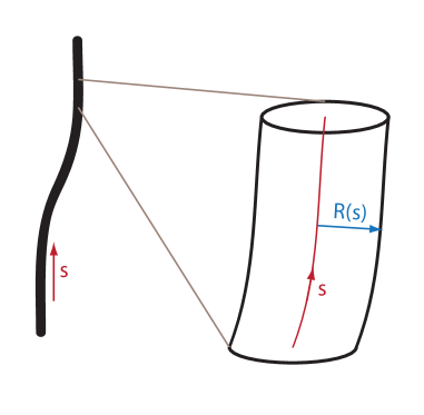
Figure 1: Schematic of a part of a discharge channel, parameterized by arc length $s$ and radius $R(s)$. The interior of the channel is filled by a mostly electrically neutral plasma providing the conductivity of the channel while the lateral walls contain most of the electric charge that is due to an overshoot of plasma species of one polarity.

Linear channel parts: radius $R$, line charge density $q$, line conductivity $\sigma$ and electric current $I$. — A schematic of a linear channel part is provided in Fig. 1. We parameterize the channel length with a longitudinal or arc length coordinate $s$, and we assume these parts to be cylindrically symmetric with a radius $R(s,t)$. The conductivity of the channel is provided by the densities $n_{e,\pm}$ and the mobilities $\mu_{e,\pm}$ of the electrons and of the positive and negative ions inside the channel, and we define a line conductivity $\sigma(s,t)$ as the integral of the conductivity over the channel cross section

$$\sigma(s,t)=\int 2\pi\;r\;dr\;\left(\mu_{e}n_{e}+\mu_{+}n_{+}+\mu_{-}n_{-}\right)(r,s,t),$$ (1)

and a line charge density $q(s,t)$ by the integral of the charge density over the channel cross section

$$q(s,t)=\int 2\pi\;r\;dr\;{\rm e}\;\left(n_{+}-n_{e}-n_{-}\right)(r,s,t),$$ (2)

where e is the elementary charge. The line conductivity is the inverse of the resistance per length, and the line charge density is the charge per length.

In general, we can assume that the radius varies slowly over the arc length $s$. The electric charge typically resides in the surface of channel. It can be assumed to be cylindrically symmetric as long as other charges stay at a distance much larger than the channel radius. According to standard electrodynamics, the electric field created by the charge of the channel is determined only by the line charge density and not by the channel radius at distances much larger than the channel radius.

The electric current $I(s,t)$ along the conducting channel is determined by Ohm’s law,

$$I(s,t)=\sigma(s,t)\;E(s,t),$$ (3)

where $E(s,t)$ is the local electric field inside the channel; here we used that the electric field inside the channel, i.e., inside the space charge layer, does essentially not change in the radial direction, and that it is oriented along the channel Ratushnaya et al. (in preparation) — otherwise the current would flow into or out of the channel walls and would change the charge content very rapidly; hence as long as charges change slowly, the field is directed along the axis.

The conservation of electrical charge implies

$$\partial_{t}q(s,t)+\partial_{s}I(s,t)=0.$$ (4)

For radius $R(s,t)$ or line conductivity $\sigma(s,t)$ particular dynamical equations could be implemented that incorporate physical understanding of the channel dynamics. Alternatively they can be considered as fixed after they have been generated by the motion of the channel head.

Head radius, charge, velocity and branching. — The charge distribution in the discharge head and channel together with the external field determine the electric field distribution at the head. The head velocity in general depends not only on the electric field in some particular spot, but on the electric field $\mathbf{E}_{enh}$ and electron density distribution in the whole ionization region at the discharge head; and the shape of this region is strongly determined by the head radius $R$. The velocity of head or tip can therefore be considered as a function of radius $R$, electric field $\mathbf{E}_{enh}$, polarity $\pm$ and of gas type and conditions,

$${\bf v}_{\rm tip}^{\pm}={\bf v}^{\pm}\Big{(}\mathbf{E}_{enh},~{}R,\mbox{ gas type and preionization}\Big{)}.$$ (5)

For the velocity of streamers in air, Naidis has suggested a particular analytic approximation in Naidis (2009).

For branching of the channel tip, an appropriate distribution as a function of the head parameters has to be found. For positive streamers in air, both experimental Briels et al. (2008a); Nijdam et al. (2008); Heijmans et al. (2013); Kanmae et al. (2012) and theoretical Luque and Ebert (2011) studies have been presented; they constitute the start of quantitative investigations.

The channel conductivity is also created at the channel tip. Particular results for ionization degrees for streamers in air will be discussed later. For leaders, also a reduced medium density due to thermal expansion contributes to increasing the electrical conductivity of the channel.

Electric field. — The electric field is given by the external field plus contributions due to the charges in the tree. In density approximation, the electric potential is given by the classical equation

$$\phi({\bf r})=\phi_{ext}({\bf r})+\frac{1}{4\pi\epsilon_{0}}\int d{\bf r}^{\prime}\;\frac{{\rm e}(n_{+}-n_{e}-n_{-})({\bf r}^{\prime})}{|{\bf r}-{\bf r}^{\prime}|}.$$ (6)

We recall that the electrical charge density ${\rm e}(n_{+}-n_{e}-n_{-})$ is nonvanishing essentially only in the walls of the channels, at the radius $R$. When approximating the channel by a line as above, the kernel in (6) has to be modified by a regularization to avoid unphysical singularities for $|{\bf r}-{\bf r}^{\prime}|\to 0$. We use

$$\phi({\bf r})=\phi_{ext}({\bf r})+\frac{1}{4\pi\epsilon_{0}}\int ds\;\frac{q(s)}{|{\bf r}-{\bf r}(s)|+R}.$$ (7)

Other kernels may be acceptable as long as they have the correct asymptotics for $|{\bf r}-{\bf r}(s)|\gg R$ but we have found problems of instability with non-monotonic kernels.

The general set-up of this model allows the implementation of approximations derived from more microscopic 3D fluid or particle models on propagation and branching of channel heads of positive or negative polarity and on the diameters and dynamically changing conductivities of the discharge channels. In this manner, the model eventually can serve as an upscaling step in a hierarchy of multiscale models for streamers, leaders, sprites, jets or any other discharge types, into which the detailed knowledge on diameters, velocities, ionization and branching rates derived on a smaller length scale can be implemented. Here we recall that, e.g., for streamers, the diameters, velocities and ionization degrees can vary by several orders of magnitude Briels et al. (2008a).

II.2 The simplest streamer tree model

In the current paper, we will make a number of assumptions to make the model as simple as possible. This will allow us to identify the key new features induced by consistent charge transport, without having to wonder whether properties are due to particular other model features.

In this simplest model, we assume that all channel parts and tips have the same time independent radius $R$ and line conductivity $\sigma$, that the streamer head velocity is proportional to the local electric field, and that branching is a Poisson process depending on the length of the streamer segment.

Together with the electric potential being fixed at the boundary of the simulation domain, and with the location of the electrode that supplies the electric current, these assumptions characterize the physical model.

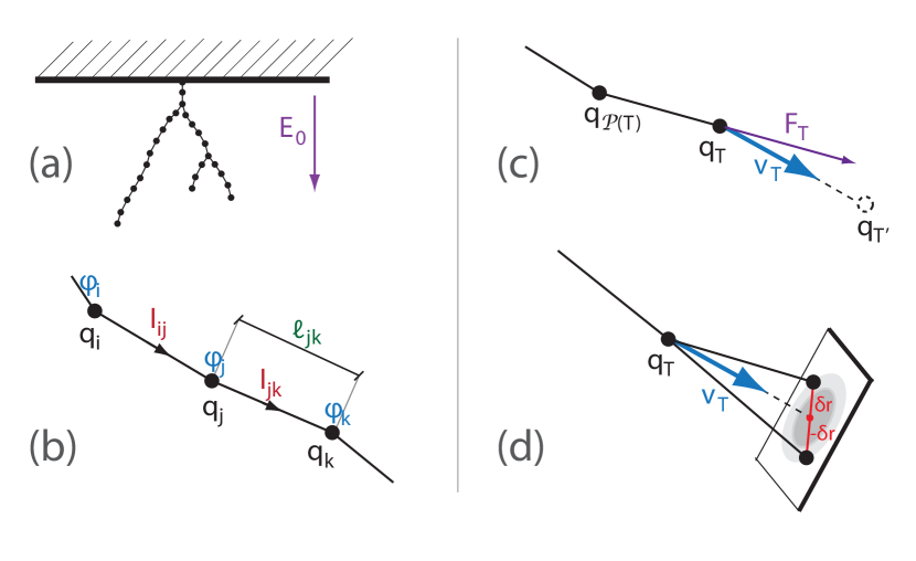
Figure 2: Scheme of the numerical implementation of the model. (a) The streamer tree is represented as a tree of nodes, each containing some charge and connected to neighbouring nodes with a finite-conductance link. (b) Each node $i$ contains a charge $q_{i}$; during the relaxation phase of the numerical simulation, charge is transported along the conductor links of length $\ell_{ij}$ by currents $I_{ij}$, changing the electric potentials $\phi_{i}$. (c) The terminal nodes of the tree advance in discrete time steps by the addition of a node further along the channel; the location of this node $T^{\prime}$ is determined by a velocity $\mathbf{v}_{T}$ determined by the local electric field at the terminal node $T$. (d) When a streamer branches, the offspring of the node $T$ consists of two nodes: each one is displaced from the straight path by a random vector $\pm\delta\mathbf{r}$ in the plane perpendicular to the original streamer path; $\delta\mathbf{r}$ is drawn from a bi-dimensional gaussian probability distribution.

II.3 Numerical implementation

We shall describe now the numerical implementation of the model described above. This numerical implementation, along with all the input files used in this articles is freely available.

As sketched in Figure 2, we replace the continuous arc lengths $s$ of the different linear channel parts by the set $i=1,\ldots,N$ of $N$ charged nodes at positions $\mathbf{r}_{i}$, each containing a time-dependent charge $q_{i}(t)$, and a time dependent electric potential $\phi_{i}(t)$ is attributed to each node. The tree evolves through two coupled mechanisms. First, due to the electric field, charge is transported along the edges. Second, each channel grows or branches at its tip according to the local conditions. In our model, we alternate between these two evolutions: to evolve our system from time $t$ to time $t+\Delta t$ we first calculate the electric field and transport the charge in the tree for an interval $\Delta t$, and then we add new nodes at the tips of existing channels, allowing some channels to branch eventually. The choice of the numerical time step $\Delta t$ is discussed in A. We describe now the steps of the simulation.

Electric field with boundary conditions. — We assume that the stem of the discharge tree is connected to an upper planar electrode located at $z=0$ that creates a constant background electric field $\mathbf{E}_{0}$. This electrode together with the set of charges $q_{i}$ with $i=1\ldots N$ within the discharge tree create an electric potential

$$\phi_{j} = \frac{1}{4\pi\epsilon_{0}}\sum_{i=-N}^{N}{\frac{q_{i}}{\ell_{ij}+R}}+\phi_{\rm ext}(\mathbf{r}_{j}),$$ (8)

$$\ell_{ij} = |{\bf r}_{i}-{\bf r}_{j}|,\quad\phi_{\rm ext}(\mathbf{r})=-\mathbf{E}_{0}\cdot\mathbf{r}$$

at the node $j$, according to equation (4). Here $i=-1\ldots-N$ parameterizes the mirror charges introduced to keep the electrode at potential zero: for each charge $q_{i}$ located at ${\bf r}_{i}=(x,y,z)$ a mirror charge $q_{-i}=-q_{i}$ is located at ${\bf r}_{-i}=(x,y,-z)$. The node $i=0$ is taken as the root of the tree; it is located at the origin, and it is discharged by the contact with the electrode. Therefore $q_{0}=0$.

For details on the numerical solution of the electrostatic problem (8), we refer to A.

Charge transport within the tree. — During the relaxation phase, electric currents flow along the conductor links according to Ohm’s law, where the current through each link is calculated from the potential difference between its two endpoints as

$$I_{ij}=\sigma E_{ij},\qquad E_{ij}=-\frac{\phi_{i}-\phi_{j}}{\ell_{ij}}.$$ (9)

Due to these currents, the charge at node $i$ changes as

$$\frac{dq_{i}}{dt}=\sum_{j\in{\mathrm{neigh}(i)}}I_{ij},$$ (10)

where $\mathrm{neigh}(i)$ stands for the set of nodes connected to $i$. For the root node $i=0$, $q_{0}=0$ is maintained because the current $I_{01}$ is exactly balanced by the current drawn from the electrode.

At each time step, we integrate the set of ordinary differential equations and (10), coupled with (II.3), from $t$ to $t+\Delta t$. In our implementation, we used the real-valued Variable-coefficient Ordinary Differential Equation (VODE) solver Brown et al. (1989).

Growth of tree tips. — Each streamer in the tree grows at its tip, and we model this growth by adding a new node $T^{\prime}$ ahead of the old terminal node $T$ after time $\Delta t$ at the location

$$\mathbf{r}_{T^{\prime}}=\mathbf{r}_{T}+\mathbf{v}_{T}\Delta t,$$ (11)

see figure 2c.

The tip velocity $\mathbf{v}_{T}$ depends on the electric field distribution around the terminal node $T$. We approximate this distribution by the electric field in the node $T$ generated by the background field and the charges of all other nodes plus the term $\mathbf{F}_{T}$

$$\mathbf{E}_{T}=\mathbf{E}_{0}+\frac{1}{4\pi\epsilon_{0}}\sum_{j\neq T}^{N}{\frac{q_{j}\mathbf{e}_{jT}}{(|\mathbf{r}_{j}-\mathbf{r}_{T}|+R)^{2}}}+\mathbf{F}_{T},$$ (12)

where $\mathbf{e}_{jT}$ is a unit vector pointing from $\mathbf{r}_{j}$ to $\mathbf{r}_{T}$.

The term $\mathbf{F}_{T}$ accounts for the contribution of the terminal node $T$. In the limit $\Delta t\to 0$, as the separation between nodes decreases, the charge contained in the terminal node becomes negligible compared with the many charges in the channel at distances shorter than $R$. For finite $\Delta t$, the term $\mathbf{F}_{T}$ accounts for the contribution of these many charges that are now summed up into the terminal charge $q_{T}$:

$$\mathbf{F}_{T}=\frac{q_{T}\mathbf{e}_{\mathcal{P}(T)T}}{4\pi\epsilon_{0}R^{2}},$$ (13)

where $\mathbf{e}_{\mathcal{P}(T)T}$ is the unit vector that points towards $T$ from its predecessor $\mathcal{P}(T)$.

We will assume that the tip velocity is proportional to $\mathbf{E}_{T}$ through a model parameter that we name head mobility, $\mu_{H}$. Since the charges that enter into equations (12) and (13) change continuously during the time interval $\Delta t$, we advance the streamer tips with a velocity that is linearly interpolated from its values at $t$ and at $t+\Delta t$:

$$\mathbf{v}_{T}=\frac{1}{2}\mu_{H}\left[\mathbf{E}_{T}(t)+\mathbf{E}_{T}\left(t+\Delta t\right)\right].$$ (14)

Assuming a linear dependence of the tip velocity with the electric field is a strong simplification that nevertheless can be easily removed to incorporate more realistic dependences. In B we study one of them, where we impose a minimum electric field for streamer propagation.

Branching. — We model streamer branching only phenomenologically. We assume that branching is a Poisson process characterized by the length $\ell_{\mathrm{branch}}$ along the streamer channel. Hence the probability that the streamer tip at $T$ branches during a time step $\Delta t$ is

$$p=v_{T}\;\Delta t/\ell_{\mathrm{branch}}$$ (15)

We always ensure that the time step $\Delta t$ is such that $p\ll 1$.

Once the algorithm has decided that a tip branches, the location of its two descendant nodes is calculated as shown in figure 2d; the locations of the two new tips $\mathbf{r}_{T^{\prime}\pm}$ are symmetrical with respect to the location of the straight path (11):

$$\mathbf{r}_{T^{\prime}\pm}=\mathbf{r}_{T}+\mathbf{v}_{T}\Delta t\pm\mathbf{\delta r},$$ (16)

where $\mathbf{\delta r}$ is a random vector in the plane perpendicular to $\mathbf{v}_{T}$ with a bi-dimensional gaussian distribution with standard deviation $\ell_{\rm sib}$.

II.4 Model parameters, specifically for positive streamers in ambient air

Parameter and symbol	Value for positive streamers in STP air
Channel radius $R$	$1\,\mathrm{mm}$
Head mobility $\mu_{H}$	$900\,\mathrm{cm^{2}V^{-1}s^{-1}}$
Line conductivity $\sigma$	$9.6\cdot 10^{-7}\,\mathrm{cm\,\Omega^{-1}}$
Branching ratio $\ell_{\mathrm{branch}}/R$	$10$
Initial separation between sibling branches $\ell_{\rm sib}/R$	$0.1$

Table 1: Parameters of our simplest model and estimated values for positive streamers in air at standard temperature and pressure.

Our model contains five dimensional parameters, the radius $R$ of the discharge channel, the mobility $\mu_{H}$ of the channel head, the line conductivity $\sigma$, the average channel length $\ell_{\rm branch}$ between two branching points, and the initial separation $\ell_{\rm sib}$ between two new branches. These parameters have to be chosen appropriately for the system under consideration, like streamers or leaders in different gases and at different pressures and temperatures.

For positive streamers in air at standard temperature and pressure we now estimate their values from phenomenological observations. These values are listed in Table 1.

Streamer radius $R$. Depending on the applied voltage, visible streamer diameters in air at standard temperature and pressure vary between a minimum of $\approx 0.12$ millimeter Nijdam et al. (2010) and 3 millimeters in the experiments of Briels et al. Briels et al. (2008a) for sharply pulsed voltages of up to 100 kV, and increase up to the order of 1 cm in the experiments of Kochkin et al. Kochkin et al. (2012) with a Marx-generator delivering MV-pulses. Due to the projection of the radiation into the 2D image plane and the nonhomogeneous excitation of emitting species in the streamer head, the radiative or visible diameter is about half of the electrodynamic diameter that parameterizes the extension of the space charge layer around the streamer tip, i.e. the visible diameter approximates the electrodynamic radius. Numerical simulations Luque et al. (2008b); Pancheshnyi et al. (2005) show radii in the range of 0.1 to 1 mm, similarly to the measurements of Briels et al. (2008a). As streamers of minimal diameter generically do not branch, we have here chosen an electrodynamic radius of $R\approx 1\,\mathrm{mm}$.

Head mobility $\mu_{H}$. It was found in experiments Briels et al. (2008a) as well as in simulations Luque et al. (2008b) that the velocity of a positive streamer strongly depends on its radius. The analysis of Naidis Naidis (2009) showed that the velocity of a uniformly translating streamer also depends on the peak electric field. This is because the peak field together with the radius determine the size of the region around the streamer head where the electric field is above the breakdown value and where the ionization grows. Naidis’ numerical data for a fixed radiative diameter of 1 mm suggest a roughly linear approximation $v\approx\mu_{H}E_{p}$, $\mu_{H}\approx 900\,\,\mathrm{cm^{2}\,V^{-1}\,s^{-1}}$, where $E_{p}$ is the peak electric field at the streamer ionization front.

Line conductivity $\sigma$. The electrical conductivity inside a streamer channel is dominated by the free electrons. Most numerical simulations Pancheshnyi et al. (2005); Dhali and Williams (1987); Kulikovsky (1997); Liu and Pasko (2004); Bourdon et al. (2007); Wormeester et al. (2010) agree on a value of about $n_{0}\approx 10^{14}\,\mathrm{cm^{-3}}$ electrons on the streamer axis, and a further analysis of the relation between peak field $E_{p}$ and ionization density $n_{0}$ behind the front can be found in Li et al. (2007). If we assume a quadratic decay of the density away from the axis up to a radius $R$, we obtain

$$\sigma=2\pi\mathrm{e}\mu n_{0}\int_{0}^{R}r\left(1-\frac{r^{2}}{R^{2}}\right)\,dr=\frac{\pi}{2}\mathrm{e}\mu n_{0}R^{2},$$ (17)

where $\mathrm{e}$ is the elementary charge, and $\mu\approx 380\,\,\mathrm{cm^{2}\,V^{-1}\,s^{-1}}$ is the electron mobility Davies et al. (1971). The expression (17) yields $\sigma=9.6\cdot 10^{-7}\,\mathrm{cm\,\Omega^{-1}}$.

Branching ratio $\ell_{\mathrm{branch}}/R$. Briels et al. Briels et al. (2008b) measured an approximately linear relationship between average branching distance and streamer radius for positive streamers in air. We use their value $\ell_{\mathrm{branch}}/R\approx 10$, where $R$ is the electrodynamic streamer radius.

Initial separation $\ell_{\rm sib}$ between sibling branches. Finally, we used the arbitrary value $0.1R$ for $\ell_{\rm sib}$. The only constraints on this value are that is is much smaller than $\ell_{\mathrm{branch}}$ and that it is of the order of $v\Delta t$, where $v$ is a typical streamer velocity. Below, we will find that the effect of the value of $\ell_{\rm sib}$ on the simulations is quite weak.

III Results of the simulations

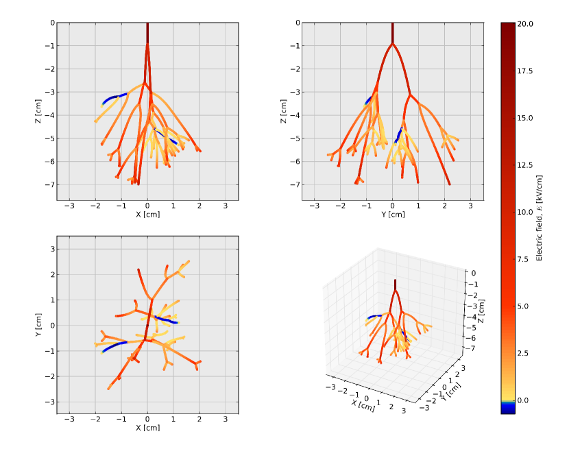
Figure 3: Simulation of a positive streamer tree in air under normal conditions in an applied field of 15 kV/cm with the parameters of Table 1. We show the projections of the streamer tree on the $xz$, $yz$ and $xy$ planes as well as a 3d plot. The snapshot corresponds to $t=80\,\mathrm{ns}$ of simulated time; at this point there are 45 streamer branches. The colors of the streamer channels indicate the internal electric field, as described in the text.

III.1 Internal electric fields

Simulation and overall structure. — Figure 3 shows a streamer tree simulated with the parameters of Table 1 and an external electric field $E_{0}=15\,\mathrm{kV/cm}$ pointing downwards. This field corresponds to about half of the classical breakdown field. We colored the edge between two connected nodes $i$ and $j$ according to the mean electric field in the link, defined as

$$E_{ij}=\frac{\phi_{i}-\phi_{j}}{\ell_{ij}}.$$ (18)

We chose the order of the labels $i$ and $j$ such that the electric field is positive in the direction of streamer propagation.

The $xz$ projection of the streamer tree in Figure 3 (upper left) has an approximately diamond shape; in the upper part the tree becomes wider at lower altitude due to the repulsion between the heads whereas in a lower part the tree gets thinner because the branches close to the center propagate faster. The diamond shape is typical in sprites Cummer et al. (2006) and in laboratory streamers Ebert et al. (2006); Kochkin et al. (2012) captured before they contact the lower electrode. In needle-plane discharges, the strong divergence of the electric field around the needle electrode produces a sharper widening of the tree during the initial stages of evolution, hence in the upper part of the discharge.

We name the discharge structure in figure 3 a collective streamer front; it can be interpreted as a “streamer of streamers.” The many positive charges at the tips of the lower channels have a role akin to the continuous space charge layer in a single streamer. Below them, they enhance the field around the center axis; above, the field is screened. In a single streamer, the charge is transported to the boundary due to the enhanced conductivity of the streamer channel; in a streamer tree, there is a coarse-grained conductivity arising from the many conductive filaments inside the tree. Figure 4 illustrates this phenomenon by plotting the electrostatic potential in a region around the streamer tree. The equipotential lines are further apart inside the tree, indicating a lower electric field, whereas they are compressed in the volume directly in front of the tree, where the electric field is significantly enhanced.

Figure 4: Electrostatic potential in the $x=0$ plane in the region surrounding the streamer tree of figure 3. In the projection of the streamer tree, we have increasingly dimmed the channels when they are further out of the $x=0$ plane.

Non-constant electric fields inside the streamer. — The average of the internal electric fields plotted on Figure 3 is close to the stability field of positive streamers Raizer (1991); Allen and Ghaffar (1995); Briels et al. (2008a) around $5\,\mathrm{kVcm^{-1}}$. However, we emphasize that the internal fields are not constant, as was assumed in previous studies on streamer coronas Pasko et al. (2000); Bondiou and Gallimberti (1994); Becerra and Cooray (2006); Arevalo and Cooray (2011). The field is stronger close to the streamer head, decaying smoothly as we move upwards in the channel. At a branching point, the field in the parent branch exceeds that of the two descendant branches. This results from charge conservation: after some transition time, the current that flows into the branching node equals the sum of the currents flowing out; since the currents are proportional to the internal fields, the fields in the descendant branches must be lower than in the parent branch.

Field reversal. — A salient feature of the fields shown in Figure 3 is that in some channels the fields have an opposite sign, transporting charge backwards. Although seemingly paradoxical, this results from some streamers outrunning others, as outlined in Figure 5. The charges in a streamer create a field $E_{ch}$ that oppose the external field $E_{0}$. Normally $E_{ch}$ and $E_{0}$ add up into an internal field weaker than the external field but with the same orientation. Suppose, however, that the streamer is overrun by a few neighbouring streamers carrying charges that screen $E_{0}$ inside the original streamer. Then only $E_{ch}$ remains inside the channel, which thus starts to discharge. In that case the streamer halts, leaving a “dead” channel behind.

However, our algorithm, as described in II.3 adds new nodes to the tree tips even for very small values of the velocity defined in (14). The resulting slow growth of these dead channels is most often irrelevant for the overall dynamics of the streamer tree but may result in unphysical behaviour, such as streamer channels slowly turning backwards.

This problem is solved by a field-velocity relation more realistic than the linear one in (14). In B we discuss the inclusion of a realistic threshold electric field for streamer propagation.

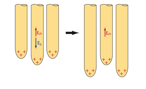
Figure 5: Inversion of the inner electric field inside a streamer channel. The driving electric field of a streamer is screened when it is overrun by neighbouring streamers. In that case the streamer dies out and the charge in the tip is driven backwards by electrostatic repulsion.

III.2 Charge distribution in the tree

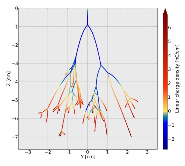
Figure 6: Charge distribution in the streamer tree of figure 3. For each node $i$ in the model we represent here $q_{i}/\ell_{\mathcal{P}(i),i}$, where $q_{i}$ is the charge in the node and $\ell_{\mathcal{P}(i),i}$ is the length of the segment ending at $i$. Note that the color scale is truncated and does not show correctly the charge density at the streamer tips, as they would dominate the plot.

The distribution of charges in the same simulation as in figure 3 appears in figure 6. To focus on the charge density inside the streamer channels, we have truncated the color scale, which would be otherwise dominated by the charges at the streamer heads.

Figure 6 shows that while the lower part of the tree, closer to the streamer tips is charged positively, the innermost segments are negatively charged. This resembles the negative charging of the upper regions of sprite streamers Luque and Ebert (2010) and arises from an analogous mechanism. The many channels in the external branches transport a large amount of charge. The fewer channels in the inner sections collect this charge, that then gets stuck due to the lower collective conductivity. Hence it brings about a negatively charged inner core in the tree.

III.3 Influence of the line conductivity

We turn now to the influence of the line conductivity $\sigma$ of the streamer channel on the propagation and shape of the streamer tree. We focus on this parameter because a straightforward dimensional analysis (see C) shows that changing the line conductivity while keeping a fixed applied electric field is equivalent, after rescaling time, to a change in the external electric field with a fixed line conductivity. Therefore the analysis described here translates directly into a study of the influence of the applied field.

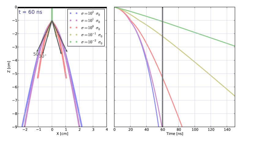
Figure 7: Influence of the line conductivity on the propagation of a singly branched streamer. For different values of the line conductivity $\sigma$, the left panel shows a snapshot of the branch at time $t=60\,\mathrm{ns}$; the right panel plots the location of the lowest point of the branch as a function of time. The vertical line marks the time of the plots in the left panel.

Branching angles. — At this point, it is helpful to suppress the randomness of the model and focus on an even simpler system. We run simulations where we impose a single branching point at $z=-1\,\mathrm{cm}$. In each of these simulations, we multiplied by a factor from $10^{-2}$ to $10^{2}$ the line conductivity discussed above and listed in Table 1, here denoted $\sigma_{0}$. Figure 7 shows the results.

The left panel of figure 7 shows the influence of the line conductivity on branching angles. Channels with a higher conductivity lead to wider branching. The reason is that charge moves more easily along the channel and then accumulates faster at the streamer tips. The electrostatic repulsion between both heads is thus stronger and they diverge more sharply.

However, figure 7 shows that this mechanism is quite weak. Although it is theoretically possible to infer the channel conductivities from branching angle measurements, such as those by Nijdam et al. Nijdam et al. (2008), the dependence seems too weak to be useful, given the natural variation and the measurement uncertainties of branching angles. In figure 7 we mark with arrows the branch-to-branch angles $30^{\circ}$ and $50^{\circ}$ from the branching point to underline that all conductivities agree with the branching angles of $(39.7\pm 13.2)^{\circ}$ reported in reference Nijdam et al. (2008) for positive streamers in air at atmospheric pressure.

Velocity. — On the right panel of figure 7 we plot the propagation distance of the streamers as a function of time for the same simulations as in the previous section. We see a significant speed-up of the propagation with increasing channel conductivity. Again, the increased charge transport and accumulation at the streamer tip explain this behaviour.

Another feature of Figure 7 is that the streamers with line conductivity $10\sigma_{0}$ and $10^{2}\sigma_{0}$ propagate almost at the same speed despite an order of magnitude difference in $\sigma$. The reason is that they approach the high-conductivity regime, where the charge distribution in the streamer adjusts instantaneously to changes in the streamer length. The reference value $\sigma_{0}$ is about a factor 10 below this limit, implying that the finite streamer conductivity is still relevant for the streamer propagation.

III.4 Influence of $\ell_{sib}$

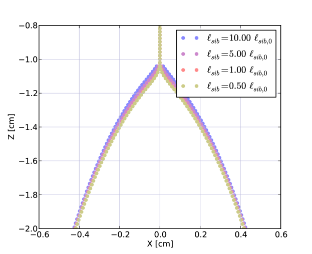
Figure 8: Four simulations with different values of $\ell_{sib}$. In the figure legend, the $\ell_{sib,0}$ refers to the value in table 1, $\ell_{sib,0}=0.1\,\mathrm{mm}$.

As we mentioned above, $\ell_{sib}$ does not substantially influence the simulations as long as it stays within reasonable physical bounds. To investigate this, we run simulations where we changed $\ell_{sib}$ from one tenth to twice the value in table 1. As in the previous section, in these simulations we forced the streamers to branch uniquely at a prescribed location $z=-1\,\mathrm{cm}$. The outcome appears in figure 8.

Simulations with very different $\ell_{sib}$ behave similarly. After a short transient, the electrostatic repulsion between the two sibling branches strongly dominates their propagation. About $1\,\mathrm{cm}$ below the branching point, the trajectories of simulations with different $\ell_{sib}$ are barely separated. We conclude that $\ell_{sib}$ which was introduced as a numerical parameter, does not influence he results much.

III.5 Reconnection

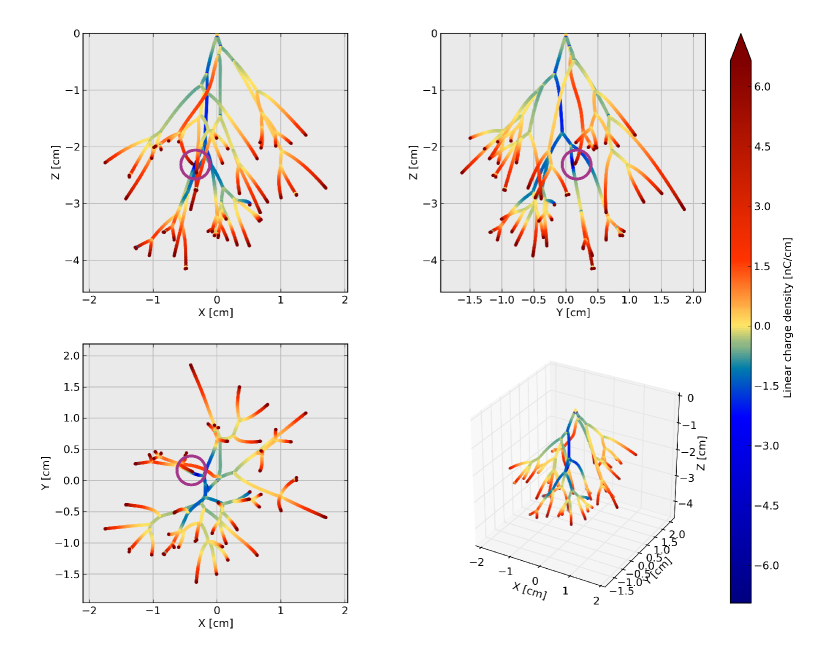
Figure 9: A reconnection event. The parameters of this simulation are those listed in Table 1. We show here a snapshot of the charge distribution at time $t=160.75\,\mathrm{ns}$. The circles mark the place of reconnection in the three projections; it is clearly seen in the $xz$ projection.

Let us now use our model to investigate the reconnection of streamer channels inside a tree. In a reconnection event, a streamer head is attracted towards a pre-existing channel. This should not be confused with streamer merging, where two streamer heads expand to form a single channel Luque et al. (2008a); Bonaventura et al. (2012).

Streamer reconnection has been observed both in laboratory discharges van Veldhuizen and Rutgers (2002); Nijdam et al. (2009) and in high-speed sprite observations Cummer et al. (2006); Stenbaek-Nielsen and McHarg (2008); Montanyà et al. (2010). Nijdam et al. Nijdam et al. (2009), reviewed the recorded examples of reconnection and extended them with new experimental data. Using stereoscopy, they were able to discriminate between actual reconnection and ambiguous observations resulting from projecting the 3d streamers into the camera plane. They concluded that reconnection of positive streamers in laboratory experiments is indeed frequent but consists in a thinner, slower streamer moving towards the channel of a thicker, faster streamer that had already contacted the cathode. After this contact, the ionized streamer channel charges negatively and attracts the streamer heads surrounding it, still positively charged. Although commonplace in the laboratory, this mechanism does not explain the observations of streamer reconnection in sprites, where a lower electrode does not exist. Here we will limit ourselves to the study of this latter kind of reconnection, where a lower electrode does not exist or is not essential. We henceforward restrict the meaning of reconnection to this type of event only. In this restricted sense, reconnection has not been unambiguously observed in laboratory experiments.

We frequently observe reconnection events in our model. Figure 9 shows an example; there, a lagging streamer is attracted to the stem of a sub-tree that has propagated much farther. This pattern is generic to all the reconnection events that we found in our simulations. The picture shows that the reason is that, as explained in section III.2, the inner branches of the tree acquire a negative charge; usually, most of the channels in that volume are similarly negatively charged but if a lagging streamer propagates through the inner sections of the tree, its positive charge is attracted and reconnects to a negative, inner branch. To put it concisely, the extremal branches are attracted towards the internal ones.

In figure 10 we zoom into the reconnection of figure 9 and plot two snapshots of the charge distribution. We see that as the head approaches the channel, it induces a significant, additional negative charge in the pre-existing channel. The relevance of these induced charges in a conductive channel was pointed out by Cummer et al. Cummer et al. (2006). Nevertheless, our simulations suggest that the initial attraction of a head towards a channel is possible only in cases where that channel has the opposite charge. The induced charges dominate only when the head is already very close to the channel.

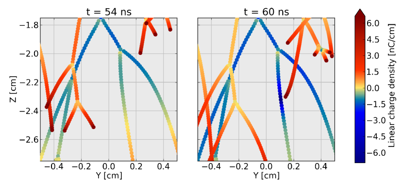
Figure 10: Zoom of the reconnection event of figure 9 at two time steps and projected onto the xz plane. A positively charged streamer head approaches a pre-existing, negative channel. The negative charge in the channel induced by the head is clearly visible in the latest time step (right panel) but an earlier time step (left panel) shows that the channel had already a negative charge before the interaction. Note also that the other branches at the right of the picture also charge negatively, even though they are not directly involved in the reconnection.

We speculate that reconnection (in our restricted sense) has not been observed in laboratory discharges because their innermost branches do not charge negatively or do not do it strongly enough. We offer two possible reasons for this. (a) That the needle-electrode geometry most often employed in the laboratory, by imposing higher and divergent electric fields around the anode, discharges the negative charges in that region faster and reduces streamer interaction. (b) That the reduced propagation length imposed by the cathode does not allow the tree enough time to reconnect. Most likely, there is a combination of both (a) and (b) at play; and finally, in the laboratory experiments Nijdam et al. (2009), only for sparse trees with less than about 50 streamers the full 3D structure can be reconstructed which gives a bias in the observations.

To investigate further whether we should expect to see streamer reconnection in laboratory experiments, we can tune the parameters in our model and make reconnection more or less likely. In particular, we may force the streamers to branch more or less frequently by varying the parameter $\ell_{branch}$. We used values from $0.35\,\mathrm{cm}$ to $5.5\,\mathrm{cm^{-1}}$ and for each value we run 10 simulations up to the time of the first reconnection. The results are plotted in figure 11.

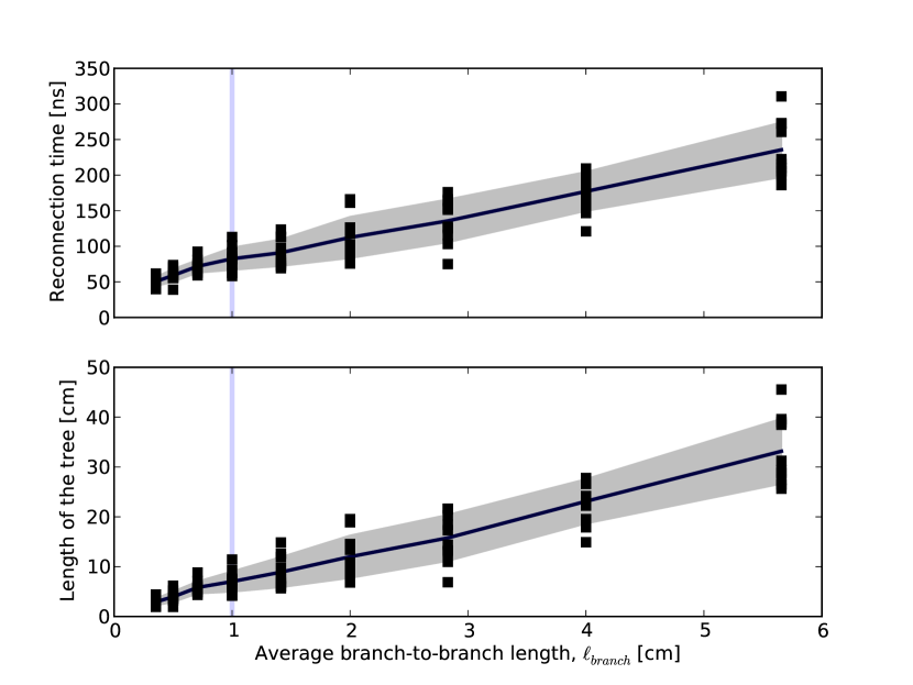
Figure 11: Dependence on the branching frequency $\ell_{branch}$ of the time to the first reconnection event and the total tree length. Here the total tree length is the largest absolute value of the $z$ coordinate of any point in the tree. For each value of $\ell_{branch}$ we run 10 simulations, plotted black squares; the continuous line represents the mean of these 10 simulations and the shaded area includes one standard deviation around the mean. The vertical line marks the standard value $\ell_{branch}=1\,\mathrm{cm}$ from table 3.

For the standard value $\ell_{branch}=2\,\mathrm{cm}$ the plot indicates that we need a gap of about $7\,\mathrm{cm}$ between electrodes to have a significant chance of observing reconnections; if $\ell_{branch}$ would increase to $2.85\,\mathrm{cm}$, one would need a gap of more than $12\,\mathrm{cm}$. Given the uncertainties and approximations in our model and point (a) discussed above we believe that laboratory discharges would also reconnect if they are given enough space.

IV Summary and conclusions

Discharge tree models constitute the highest level in space in the hierarchy of electrical discharge models. While in the past they were frequently based on phenomenological assumptions, we here present a model that rests on results and insights from fluid models, which in turn depend on the micro-physics of collisions described by particle or Boltzmann-equation models. As P.W. Anderson famously remarked Anderson (1972), each new level in such a hierarchy usually contains nontrivial, sometimes surprising, physics that are not immediately apparent from our understanding of the lower levels.

Here we have shown that even the simplest tree model with self-consistent charge transport leads to new insights into the distribution of charges and electric fields and into the process of streamer reconnection. Our model also reveals the qualitative self-similar nature of collective streamer fronts, where the full structure can be seen as a “streamer of streamers”, i.e., a scaled-up analogue of each of the streamers that compose it.

Clearly many elements of streamer physics have not been incorporated here into our model. A non-exhaustive list includes the dynamical selection of streamer diameters, the different ionization levels created in the streamer head depending on the field enhancement, and the changes in the channel conductivity due to attachment processes, the extension to negative streamers and to the gradient in air density experienced by sprite streamers in the upper atmosphere. Forthcoming investigations shall address these issues.

Appendix A Notes on the numerical implementation

A.1 Convergence of numerical time stepping

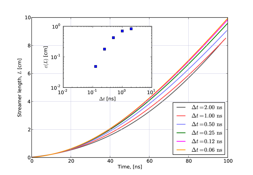
Figure 12: Convergence of the model simulations with decreasing time step $\Delta t$. The main figure shows the evolution of the streamer length with $E_{0}=15\,\mathrm{kV/cm}$ for different time steps. The inset plots the estimated error of each simulation as a function of $\Delta t$. Here $\varepsilon(L)$ is the root mean square of the difference between streamer lengths of a simulation and the most accurate simulation, $\Delta t=0.06\,\mathrm{ns}$.

A necessary condition for the numerical calculation of the model is that it converges for decreasing time step $\Delta t$. To check this, we run deterministic simulations (with $\ell_{\mathrm{branch}}=0$) with an external electric field $E_{0}=15\,\mathrm{kV/cm}$ and various $\Delta t$. Figure 12 shows the length of the streamer channel as a function of time; the simulations converge to a solution once the time steps are shorter than about $0.25\,\mathrm{ns}$.

Therefore in all simulations in this paper we use $\Delta t=0.25\,\mathrm{ns}$.

A.2 Numerical solution of the electrostatic problem

We are calculating all interactions between pairs of charged nodes and therefore our computation time scales as $O(N^{2})$. This is the main limitation in the size of trees that we can efficiently simulate. To overcome this limitation we also implemented the Fast Multipolar Method (FMM) which is able to solve the electrostatic problem with $O(N)$ computations up to an arbitrarily good approximation. However, the kernel in (II.3) is not the Poisson kernel for $R\neq 0$ and although we restricted the FMM only for distant interactions with $r_{ij}\gg R$, we run into problems around the cutoff. Besides, we found that due to the overhead of the FMM, it was advantageous only for $N$ larger than a few thousand and all the simulations reported here are below that threshold. Each of the simulations that we show took a few hours in a modern desktop computer.

Appendix B An improved model for the propagation of streamer tips

For the sake of simplicity we have assumed a linear dependence of the velocity with the electric field at the streamer tips. As we discussed in section 4, often this leads to slow streamers that keep propagating even when the surrounding electric field is very small. This contradicts both experimental observations and our theoretical understanding, where impact ionization is essential for streamer propagation. A more realistic model must include a minimum field for streamer propagation.

Taking an electrodynamic streamer radius $R=1\,\mathrm{mm}$ ($\sim$ radiation diameter), the analytical calculations in Naidis (2009) are well fitted by

$$v_{T}=\mu_{H}\max\left(0,E_{T}-E_{min}\right),$$ (19)

where the head mobility is now $\mu_{H}=3200\,\mathrm{cm^{2}V^{-1}s^{-1}}$ and the threshold field for propagation is $E_{min}=100\,\mathrm{kV/cm}$.

However, (19) presents a new problem in our plane-electrode geometry. If the applied field $E_{0}$ is lower than $E_{min}$, the tree will not start to propagate by itself. The natural solution is to implement a needle-plane geometry; here we simulated a 1 cm-needle by starting the tree from a vertical chain of 10 nodes separated by 1 mm. With $E_{0}=15\,\mathrm{kV/cm}$ this was enough to initiate a tree.

In figure 13 we show the tree created in a simulation where head velocities are as in (19). All other parameters are the same as in figure 3 in the main text. The most remarkable feature in the tree of figure 13 is the multitude of short channels that punctuate the trails of longer streamers. Often, these channels are so short that they are seen only as a sudden change in the direction of the branch. Both short branches and apparent changes in streamer direction are observed in laboratory photographs of streamer trees; they are very common in nitrogen discharges but they also appear in air (see e.g. figure 1 in reference Briels et al. (2008c)).

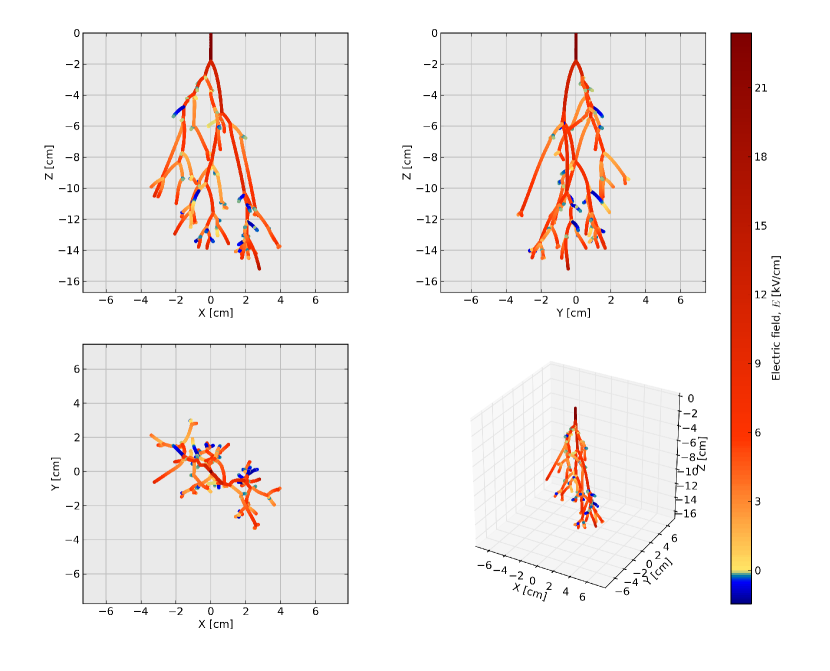
Figure 13: Streamer tree with tips growing according to equation (19) in the text; all other parameters are the same as in figure 3, listed in table 1. Here we show a snapshot of the internal electric fields at time $t=125\,\mathrm{ns}$.

Appendix C Dimensional analysis of the model

The dimensional quantities of our model are those listed in Table 1 plus the vacuum permittivity $\epsilon_{0}=8.85\cdot 10^{-14}\,\mathrm{CV^{-1}cm^{-1}}$. Straightforward dimensional analysis leads to the characteristic scales listed on table 2. Note that the characteristic scales follow the Townsend scaling laws Ebert et al. (2010); our results can be rescaled to any gas density.

A remarkable feature of table 2 is the high value of the characteristic electric field, $\mathcal{E}=2260\,\mathrm{kV/cm}$. This value is much higher than what is commonly observed in atmospheric pressure streamers and also in our simulations. The reason is that $\mathcal{E}$ defines the electric field created by a typical electron density confined in a typical streamer volume. However, $\mathcal{E}$ does not take into account that most of the electron density is screened by a similar density of positive ions. The weak-field limit in our model, where all electric fields are much lower that $\mathcal{E}$, is therefore equivalent to quasi-neutrality; namely that the electron and ion densities $n_{e}$, $n_{\pm}$ satisfy $|n_{+}-n_{-}-n_{e}|\ll n_{e}$.

One can use the values in Table 2 to derive a dimensionless model where the only parameters are $R/\ell_{\mathrm{branch}}\approx 1/20$ Briels et al. (2008b) and, for a given external electric field $E_{0}$, the ratio $E_{0}/\mathcal{E}$. An immediate consequence is that these two dimensionless quantities fully determine the geometric properties of a streamer tree, such as angles and length ratios.

Magnitude	Characteristic scale	Value at atmospheric pressure
Length	$R$	$1\,\mathrm{mm}$
Electric field	$\mathcal{E}=\sigma/4\pi\epsilon_{0}\mu_{H}R$	$2260\,\mathrm{kV/cm}$
Velocity	$v=\mu_{H}\mathcal{E}$	$2\cdot 10^{7}\,\mathrm{m/s}$
Time	$\tau=R/v$	$0.12\,\mathrm{ns}$

Table 2: Characteristic scales of the streamer tree model.

References

- Rakov and Uman (2003) V. A. Rakov and M. A. Uman, Lightning (Cambridge University Press, Cambridge, UK, 2003).
- Wescott et al. (1995) E. M. Wescott, D. Sentman, D. Osborne, D. Hampton, and M. Heavner, Geophys. Res. Lett. 22, 1209 (1995).
- Su et al. (2003) H. T. Su, R. R. Hsu, A. B. Chen, Y. C. Wang, W. S. Hsiao, W. C. Lai, L. C. Lee, M. Sato, and H. Fukunishi, Nature (London) 423, 974 (2003).
- Franz et al. (1990) R. C. Franz, R. J. Nemzek, and J. R. Winckler, Science 249, 48 (1990).
- Li et al. (2012a) C. Li, U. Ebert, and W. Hundsdorfer, J. Comput. Phys. 231, 1020 (2012a), eprint 1103.2148.
- Eichwald et al. (2008) O. Eichwald, O. Ducasse, D. Dubois, A. Abahazem, N. Merbahi, M. Benhenni, and M. Yousfi, J. Phys. D 41, 234002 (2008).
- Pancheshnyi et al. (2005) S. Pancheshnyi, M. Nudnova, and A. Starikovskii, Phys. Rev. E 71, 016407 (2005).
- Qin et al. (2012) J. Qin, S. Celestin, and V. P. Pasko, Geophys. Res. Lett. 39, L05810 (2012).
- Liu (2010) N. Liu, Geophys. Res. Lett. 37, L04102 (2010).
- Luque and Ebert (2012) A. Luque and U. Ebert, J. Comput. Phys. 231, 904 (2012).
- Li et al. (2012b) C. Li, J. Teunissen, M. Nool, W. Hundsdorfer, and U. Ebert, Plasma Sour. Sci. Technol. 21, 055019 (2012b), eprint 1203.5035.
- Luque and Ebert (2011) A. Luque and U. Ebert, Phys. Rev. E 84, 046411 (2011), eprint 1102.1287.
- Luque et al. (2008a) A. Luque, U. Ebert, and W. Hundsdorfer, Phys. Rev. Lett. 101, 075005 (2008a), eprint 0712.2774.
- Bonaventura et al. (2012) Z. Bonaventura, M. Duarte, A. Bourdon, and M. Massot, Plasma Sour. Sci. Technol. 21, 052001 (2012), eprint 1208.0114.
- Raizer (1991) Y. P. Raizer, Gas Discharge Physics (Springer-Verlag, Berlin, Germany, 1991).
- Bondiou and Gallimberti (1994) A. Bondiou and I. Gallimberti, J. Phys. D 27, 1252 (1994).
- Kochkin et al. (2012) P. O. Kochkin, C. V. Nguyen, A. P. J. van Deursen, and U. Ebert, J. Phys. D 45, 425202 (2012), eprint 1208.5899.
- Niemeyer et al. (1984) L. Niemeyer, L. Pietronero, and H. J. Wiesmann, Phys. Rev. Lett. 52, 1033 (1984).
- Akyuz et al. (2003) M. Akyuz, A. Larsson, V. Cooray, and G. Strandberg, J. Electrost. 59, 115 (2003), ISSN 0304-3886.
- Goelian et al. (1997) N. Goelian, P. Lalande, A. Bondiou-Clergerie, G. L. Bacchiega, A. Gazzani, and I. Gallimberti, J. Phys. D 30, 2441 (1997).
- Becerra and Cooray (2006) M. Becerra and V. Cooray, J. Phys. D 39, 3708 (2006).
- Arevalo and Cooray (2011) L. Arevalo and V. Cooray, J. Phys. D 44, 315204 (2011).
- Pasko et al. (2000) V. P. Pasko, U. S. Inan, and T. F. Bell, Geophys. Res. Lett. 27, 497 (2000).
- Allen and Ghaffar (1995) N. L. Allen and A. Ghaffar, J. Phys. D 28, 331 (1995).
- Gallimberti (1972) I. Gallimberti, J. Phys. D 5, 2179 (1972).
- Gallimberti (1979) I. Gallimberti, Journal de Physique 40, C7 (1979).
- Bazelyan and Raizer (2010) E. Bazelyan and Y. Raizer, Lightning Physics and Lightning Protection (Institute of Physics Publishing, Bristol, UK, 2010).
- Dhali and Williams (1987) S. K. Dhali and P. F. Williams, J. Appl. Phys. 62, 4696 (1987).
- Luque and Ebert (2010) A. Luque and U. Ebert, Geophys. Res. Lett. 37, L06806 (2010).
- Luque and Gordillo-Vázquez (2011) A. Luque and F. J. Gordillo-Vázquez, Geophys. Res. Lett. 38, L04808 (2011).
- Gordillo-Vázquez and Luque (2010) F. J. Gordillo-Vázquez and A. Luque, Geophys. Res. Lett. 37, L16809 (2010).
- Noskov et al. (2001) M. D. Noskov, M. Sack, A. S. Malinovski, and A. J. Schwab, J. Phys. D 34, 1389 (2001).
- Dissado and Sweeney (1993) L. A. Dissado and P. J. J. Sweeney, Phys. Rev. B 48, 16261 (1993).
- Ratushnaya et al. (in preparation) V. Ratushnaya, A. Luque, and U. Ebert (in preparation).
- Naidis (2009) G. V. Naidis, Phys. Rev. E 79, 057401 (2009).
- Briels et al. (2008a) T. M. P. Briels, J. Kos, G. J. J. Winands, E. M. van Veldhuizen, and U. Ebert, J. Phys. D 41, 234004 (2008a), eprint 0805.1376.
- Nijdam et al. (2008) S. Nijdam, J. S. Moerman, T. M. P. Briels, E. M. van Veldhuizen, and U. Ebert, Appl. Phys. Lett. 92, 101502 (2008), eprint 0802.3639.
- Heijmans et al. (2013) L. C. J. Heijmans, S. Nijdam, E. M. van Veldhuizen, and U. Ebert (2013), eprint 1305.1142.
- Kanmae et al. (2012) T. Kanmae, H. C. Stenbaek-Nielsen, M. G. McHarg, and R. K. Haaland, J. Phys. D 45, 275203 (2012).
- Brown et al. (1989) P. N. Brown, G. D. Byrne, and A. C. Hindmarsh, SIAM J. Sci. Stat. Comput. 10, 1038 (1989).
- Nijdam et al. (2010) S. Nijdam, F. M. J. H. van de Wetering, R. Blanc, E. M. van Veldhuizen, and U. Ebert, J. Phys. D 43, 145204 (2010), eprint 0912.0894.
- Luque et al. (2008b) A. Luque, V. Ratushnaya, and U. Ebert, J. Phys. D 41, 234005 (2008b), eprint 0804.3539.
- Kulikovsky (1997) A. A. Kulikovsky, J. Phys. D 30, 441 (1997).
- Liu and Pasko (2004) N. Liu and V. P. Pasko, J. Geophys. Res. (Space Phys) 109, A04301 (2004).
- Bourdon et al. (2007) A. Bourdon, V. P. Pasko, N. Y. Liu, S. Célestin, P. Ségur, and E. Marode, Plasma Sour. Sci. Technol. 16, 656 (2007).
- Wormeester et al. (2010) G. Wormeester, S. Pancheshnyi, A. Luque, S. Nijdam, and U. Ebert, J. Phys. D 43, 505201 (2010), eprint 1008.3309.
- Li et al. (2007) C. Li, W. J. M. Brok, U. Ebert, and J. J. A. M. van der Mullen, J. Appl. Phys. 101, 123305 (2007), eprint physics/0702129.
- Davies et al. (1971) A. J. Davies, C. Davies, and C. Evans, Proc. IEE 118, 816 (1971), ISSN 0020-3270.
- Briels et al. (2008b) T. M. P. Briels, E. M. van Veldhuizen, and U. Ebert, J. Phys. D 41, 234008 (2008b), eprint 0805.1364.
- Cummer et al. (2006) S. A. Cummer, N. Jaugey, J. Li, W. A. Lyons, T. E. Nelson, and E. A. Gerken, Geophys. Res. Lett. 33, L04104 (2006).
- Ebert et al. (2006) U. Ebert, C. Montijn, T. M. P. Briels, W. Hundsdorfer, B. Meulenbroek, A. Rocco, and E. M. van Veldhuizen, Plasma Sour. Sci. Technol. 15, 118 (2006), eprint physics/0604023.
- van Veldhuizen and Rutgers (2002) E. M. van Veldhuizen and W. R. Rutgers, J. Phys. D 35, 2169 (2002).
- Nijdam et al. (2009) S. Nijdam, C. G. C. Geurts, E. M. van Veldhuizen, and U. Ebert, J. Phys. D 42, 045201 (2009), eprint 0810.4443.
- Stenbaek-Nielsen and McHarg (2008) H. C. Stenbaek-Nielsen and M. G. McHarg, J. Phys. D 41, 234009 (2008).
- Montanyà et al. (2010) J. Montanyà, O. van der Velde, D. Romero, V. March, G. Solà, N. Pineda, M. Arrayas, J. L. Trueba, V. Reglero, and S. Soula, J. Geophys. Res. (Atmos.) 115, A00E18 (2010).
- Anderson (1972) P. W. Anderson, Science 177, 393 (1972).
- Briels et al. (2008c) T. M. P. Briels, E. M. van Veldhuizen, and U. Ebert, IEEE Trans. Plasma Sci. 36, 906 (2008c), eprint 0802.0380.
- Ebert et al. (2010) U. Ebert, S. Nijdam, C. Li, A. Luque, T. Briels, and E. van Veldhuizen, J. Geophys. Res. (Space Phys) 115, A00E43 (2010), eprint 1002.0070.