ESTIMATES FOR THE ABELIAN $Z^{\prime}$ COUPLINGS FROM THE LHC DATA

Abstract

In this paper, we investigate the Drell-Yan process with the intermediate heavy $Z^{\prime}$ boson. We use a general approach to the Abelian $Z^{\prime}$ that utilizes the renormalization-group relations between the $Z^{\prime}$ couplings and allows to reduce the number of unknown $Z^{\prime}$ parameters significantly. In a newly proposed strategy, we estimate the LHC-driven constraints for the $Z^{\prime}$ couplings to lepton and quark vector currents. To do this, we calculate the $Z^{\prime}$-related contribution in the narrow-width approximation and compare the obtained values to the experimental data presented by the ATLAS and CMS collaborations. Our method allows to estimate the values of $Z^{\prime}$ couplings to the $u$ and $d$ quarks and to final-state leptons.

I Introduction

Searching for new particles beyond the Standard Model (SM) is an important part of experiments at the Large Hadron Collider. Among the scenarios of new physics a heavy neutral vector boson ($Z^{\prime}$ boson) is one of the most promising intermediate states to be detected in hadron scattering processes in the annihilation channel. This particle resides in popular grand unification theories (GUTs) and other models with extended gauge sector (see Refs. leike ; Lang08 ; Rizzo06 for review). Considering a couple of $Z^{\prime}$ models, current experiments constrain its mass to be no less than 1-3 TeV ATLAS:2013NW ; CMS:2013NW . At the LHC $Z^{\prime}$ bosons could be discovered in the Drell-Yan process through deviations of the cross-section from the predicted SM background.

Unfortunately, observables in experiments at hadron colliders are calculated with significant theoretical uncertainties, that arise from the parton model of hadrons. In this situation one can only hope to discover the most prominent signals. This is the reason for LHC collaborations to pay special attention to searching for narrow $Z^{\prime}$ resonances.

In general, to accurately describe the $Z^{\prime}$ contribution to the Drell-Yan process and to take into account the possible interference effects Boos_ea_1 ; Boos_ea_2 , we have to consider scattering amplitudes with intermediate virtual states. This allows to derive few-parametric observables suitable for data fitting PankovTsytrinov:2009prd ; GulovKozh:2012obs . But if the resonance is estimated to be narrow, then one can describe it in a more simple way by a small number of $Z^{\prime}$ production and decay characteristics. In this approach it is only needed to set the $Z^{\prime}$ mass, the production cross-section, and the total and partial decay widths. Being quite simple, such a scheme at the same time could give estimations of $Z^{\prime}$ couplings to the SM fields based on the current experimental data.

It is possible to calculate effects of $Z^{\prime}$ boson in details for each specific GUT model. Such model-dependent estimates are widely presented in the literature Erler:2009jh ; aguila ; Erler:2010arxiv ; Corcella:models2013 ; PankovAndreev:models2012 ; PankovAndreev:models2013 ; Cao:models2012 ; Basso:models2012 ; Belyaev:models2013 . Some set of popular $E_{6}$-based models and left-right models is usually considered in this approach. However, probing the set one can still miss the actual $Z^{\prime}$ model. Therefore, it is useful to complement the model-dependent $Z^{\prime}$ searches by some kind of model-independent analysis (e.g. as in Ref. Eboli:indep2012 ). Lots of the usually considered models belong to the models with the so-called Abelian $Z^{\prime}$ boson. The Abelian $Z^{\prime}$ is usually understood as an effective additional $U(1)$ gauge state at energies of order of several TeVs, which obtains its heavy mass beyond the scope of the SM. Such kind of $Z^{\prime}$ boson is characterized by specific relations between its couplings to SM particles. The relations were derived in Refs. Gulov:2000eh ; Gulov:1999ry . They cover models satisfying the following conditions: 1) only one heavy neutral vector boson could be recognized at energies of modern colliders, whereas other possible heavy bosons are decoupled at essentially larger mass scales; 2) the $Z^{\prime}$ boson is decoupled at low energies and can be phenomenologically described by an effective Lagrangian leike ; Lang08 ; Rizzo06 ; 3) the underlying theory matches with either one- or two-Higgs-doublet standard model at low energies; 4) the SM gauge group is a subgroup of the gauge group of the underlying theory; 5) $Z^{\prime}$ boson is described by an effective additional $U(1)$ gauge state at low energies. While the relations are not model-independent in the most broad sense, they can be referred as applicable to a wide set of specific models. Among the popular models discussed in the literature, the left-right models and the $E_{6}$ models belong to this set. Nevertheless, it does not mean that the approach is designed and applicable only to those models.

It follows from the mentioned relations that the Abelian $Z^{\prime}$ couplings to the left-handed fermion currents within any SM doublet are the same and that the absolute value of the $Z^{\prime}$ couplings to the axial-vector currents for all the massive SM fermions is universal (see Refs. GulovSkalozub:2009review ; GulovSkalozub:2010ijmpa for details). The relations reduce significantly the number of unknown $Z^{\prime}$ parameters and leave some of them arbitrary, therefore allowing analysis of experimental data complementary to the common model-dependent approach. For instance, some Abelian $Z^{\prime}$ hints were found in LEP data GulovSkalozub:2010ijmpa .

In Ref. GulovKozhushko:2011ijmpa two different estimates both for the $Z^{\prime}$ production cross section at the LHC and the $Z^{\prime}$ decay width were presented. Those are the 95% CL estimate, where all the $Z^{\prime}$ coupling constants are varied in their 95% confidence level (CL) intervals derived by LEP data, and the maximum-likelihood estimate, where the $Z^{\prime}$ coupling to axial-vector currents is set to its mean value from experimental data, $a/m_{Z^{\prime}}\simeq\pm 0.14\mathrm{~{}TeV}^{-1}$, and the fermionic couplings $v_{f}$ are varied in their 95% CL intervals. It was shown that in case of the maximum-likelihood estimate at $Z^{\prime}$ masses up to 1.5 TeV the narrow-width approximation (NWA) is applicable, and therefore it is possible to calculate the $Z^{\prime}$ contribution to the Drell-Yan cross section as $\sigma(pp\to Z^{\prime})\times BR(Z^{\prime}\to l^{+}l^{-})$. However, this is not the case for higher $Z^{\prime}$ mass region, namely, at $m_{Z^{\prime}}$ $\sim$ 2-3 TeV, which has recently been explored by the LHC collaborations ATLAS:2013NW ; CMS:2013NW . In this region the NWA condition $\Gamma_{Z^{\prime}}^{2}/m_{Z^{\prime}}^{2}\ll 1$ for the maximum-likelihood estimate is not met. The reason is that even in case of this very optimistic scenario the intervals for the vector couplings are still too wide. Since the LHC collaborations present their results calculated in the NWA, then to be able to obtain estimates of the $Z^{\prime}$ contribution to the Drell-Yan process at the LHC and compare them with the currently available data, we need to change our estimation strategy.

In our present investigation we use the relations for the Abelian $Z^{\prime}$ couplings to estimate the Abelian $Z^{\prime}$ production in the Drell-Yan process. We compare the obtained cross section to the current LHC bounds. This allows us to constrain $Z^{\prime}$ couplings. It also shows how far the LHC will potentially advance the $Z^{\prime}$ searches compared to the LEP.

In Section 2 we provide all necessary information about the $Z^{\prime}$ boson and the used relations between couplings. Section 3 contains some details regarding $Z^{\prime}$ production and decay at the LHC. In Section 4 our estimation strategy is presented. In Section 5 we discuss the obtained results.

II $Z^{\prime}$ parameterization

In the present paper we use the following effective Lagrangian to describe $Z^{\prime}$ couplings to the axial-vector and vector fermion currents:

$${\cal L}_{Z\bar{f}f} = \frac{1}{2}Z_{\mu}\bar{f}\gamma^{\mu}\left[(v^{\mathrm{SM}}_{fZ}+\gamma^{5}a^{\mathrm{SM}}_{fZ})\cos\theta_{0}+(v_{f}+\gamma^{5}a_{f})\sin\theta_{0}\right]f,$$

$${\cal L}_{Z^{\prime}\bar{f}f} = \frac{1}{2}Z^{\prime}_{\mu}\bar{f}\gamma^{\mu}\left[(v_{f}+\gamma^{5}a_{f})\cos\theta_{0}-(v^{\mathrm{SM}}_{fZ}+\gamma^{5}a^{\mathrm{SM}}_{fZ})\sin\theta_{0}\right]f,$$ (1)

where $f$ is an arbitrary SM fermion state; $a_{f}$ and $v_{f}$ are the $Z^{\prime}$ couplings to the axial-vector and vector fermion currents; $\theta_{0}$ is the $Z$–$Z^{\prime}$ mixing angle; $v^{\mathrm{SM}}_{fZ}$, $a^{\mathrm{SM}}_{fZ}$ are the SM couplings of the $Z$-boson. The commonly considered $Z^{\prime}$ gauge coupling $\tilde{g}$ is included into $a_{f}$ and $v_{f}$.

This popular parameterization follows from a number of natural conditions. First of all, the $Z^{\prime}$ interactions of renormalizable types are expected to be dominant. The non-renormalizable interactions that are generated at high energies due to radiation corrections are suppressed by $1/m_{Z^{\prime}}$ (or by other heavier scales $1/\Lambda_{i}\ll 1/m_{Z^{\prime}}$) at low energies $\sim m_{W}$ and therefore they can be neglected.

We also assume the conditions listed in the Introduction in order to use the relations between the Abelian $Z^{\prime}$ couplings. In particular, the SM gauge group ${\rm SU}(2)_{L}\times{\rm U}(1)_{Y}$ is considered as a subgroup of the GUT group. In this case, a product of the SM subgroup generators is a linear combination of these generators. Consequently, all the structure constants that connect the two SM gauge bosons with $Z^{\prime}$ have to be zero, and at the tree-level $Z^{\prime}$ interactions to the SM gauge fields are possible due to a $Z$–$Z^{\prime}$ mixing only.

To calculate the $Z^{\prime}$ contribution to the Drell-Yan process, we also need to parameterize the $Z^{\prime}$ interactions with the SM scalar and vector fields. The explicit Lagrangian describing $Z^{\prime}$ couplings to all the SM fields can be found in Ref. GulovKozhushko:2011ijmpa .

The parameters $a_{f}$, $v_{f}$, and $\theta_{0}$ could be obtained from experimental data. In a particular model, one has some specific values for some of them. If the model is unknown, all the parameters are potentially arbitrary numbers. If one assumes that the underlying extended model is renormalizable, then, as was shown in Refs. Gulov:2000eh ; Gulov:1999ry , there is a relation between these parameters:

$$v_{f}-a_{f}=v_{f^{*}}-a_{f^{*}},\qquad a_{f}=T_{3f}\tilde{g}\tilde{Y}_{\phi}.$$ (2)

Here, $f$ and $f^{*}$ are the components of the $SU(2)_{L}$ fermion doublet ($l^{*}=\nu_{l},\nu^{*}=l,q^{*}_{u}=q_{d}$, and $q^{*}_{d}=q_{u}$), $T_{3f}$ is the third component of weak isospin (1/2 for “up”-type fermions, -1/2 for “down”-type fermions), and $\tilde{g}\tilde{Y}_{\phi}$ determines $Z^{\prime}$ couplings to the SM scalar fields and the $Z$–$Z^{\prime}$ mixing angle $\theta_{0}$ in (II), which is expressed as:

$$\tan 2\theta_{0}=\tilde{g}\tilde{Y}_{\phi}\frac{\sin\theta_{W}\cos\theta_{W}}{\sqrt{4\pi\alpha_{\rm em}}}\frac{m_{Z}^{2}}{m_{Z^{\prime}}^{2}}.$$ (3)

As it was argued in Refs. GulovSkalozub:2009review ; GulovSkalozub:2010ijmpa , the relations (2) hold in a set of popular models with the Abelian $Z^{\prime}$ boson based on the ${\rm E}_{6}$ group (the so called LR, $\chi$-$\psi$ models). However, one could also think about models beyond the commonly used list of models.

Let us note that the couplings of the Abelian $Z^{\prime}$ to the axial-vector fermion currents are described by a universal absolute value. Therefore we introduce the notation

$$a=a_{d}=a_{e^{-}}=-a_{u}=-a_{\nu}.$$ (4)

From Eq. (2) it follows, that this value $a$ is proportional to the $Z^{\prime}$ coupling to scalar fields. By substituting Eqs. (2) and (4) into Eq. (3) we obtain

$$\theta_{0}\approx-2a\frac{\sin\theta_{W}\cos\theta_{W}}{\sqrt{4\pi\alpha_{\rm em}}}\frac{m_{Z}^{2}}{m_{Z^{\prime}}^{2}}.$$ (5)

Thus the $Z$–$Z^{\prime}$ mixing angle $\theta_{0}$ is also determined by the axial-vector coupling. For further calculations we use $\alpha_{\rm em}=1/128.9$, $\sin^{2}\theta_{W}=0.2304$.

It can be seen from (2), that for each fermion doublet only one vector coupling is independent:

$$v_{f_{d}}=v_{f_{u}}+2a.$$ (6)

In total, the $Z^{\prime}$ interactions with the SM particles can be parameterized by seven independent couplings: $a$, $v_{u}$, $v_{c}$, $v_{t}$, $v_{e}$, $v_{\mu}$, $v_{\tau}$.

In Refs. GulovSkalozub:2009review ; GulovSkalozub:2010ijmpa the limits on $Z^{\prime}$ couplings from the LEP I and LEP II data were obtained. One can interpret those limits as some hints of $Z^{\prime}$ boson at 1-2$\sigma$ CL. Namely, the couplings $a$ and $v_{e}$ show non-zero maximum-likelihood (ML) values. The constraints on the axial-vector coupling $a$ come from the LEP I data (through the mixing angle) and from the LEP II data on the $e^{+}e^{-}\to\mu^{+}\mu^{-},\tau^{+}\tau^{-}$ scattering. The corresponding ML values lie very close to each other. In our estimates we use the value

$$a_{\mathrm{ML}}^{2}/m_{Z^{\prime}}^{2}=1.97\times 10^{-2}\ \mathrm{TeV}^{-2}.$$ (7)

The electron vector coupling $v_{e}$ is constrained at 95% CL by the $e^{+}e^{-}\to e^{+}e^{-}$ data from LEP II (see discussion in Refs. GulovSkalozub:2009review ; GulovKozhushko:2011ijmpa ):

$$6.07\times 10^{-2}\ \mathrm{TeV}^{-2}<{v}_{e}^{2}/m_{Z^{\prime}}^{2}<2.56\times 10^{-1}\ \mathrm{TeV}^{-2}.$$ (8)

These constraints seem to be less stable, so we will use them only to compare our final results avoiding taking them into account in calculations.

There are no significant constraints on the other $Z^{\prime}$ coupling constants from the existing data.

III $Z^{\prime}$ production at the LHC

At the LHC $Z^{\prime}$ bosons are expected to be produced in proton-proton collisions: $pp\to Z^{\prime}$. At the parton level this process is described by the $Z^{\prime}$ production in the quark-antiquark pair annihilation, $q\bar{q}\to Z^{\prime}$ (Fig. 1). The cross-section of the $pp\to Z^{\prime}$ process is obtained by integrating the partonic cross-section $\sigma_{q\bar{q}\to Z^{\prime}}$ with the parton distribution functions (PDFs):

$$\sigma_{AB} = \sum_{q,\bar{q}}\int_{0}^{1}dx_{q}\int_{0}^{1}dx_{\bar{q}}\,f_{q,A}(x_{q},\mu_{R},\mu_{F})f_{\bar{q},B}(x_{\bar{q}},\mu_{R},\mu_{F})$$ (9)

$$\times\sigma_{q\bar{q}\to Z^{\prime}}(m_{Z^{\prime}},x_{q}k_{A},x_{\bar{q}}k_{B}),$$

where $A$, $B$ mark the interacting hadrons (protons in our case) with the four-momenta $k_{A}$, $k_{B}$; $f_{q,A}$ is the parton distribution function for the parton $q$ in the hadron $A$ with the momentum fraction $x_{q}$ at the renormalization scale $\mu_{R}$ and factorization scale $\mu_{F}$. We use the parton distribution functions provided by the MSTW PDF package mstw .

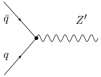
Figure 1: $Z^{\prime}$ production at the parton level.

The production cross-section includes quadratic combinations of the $Z^{\prime}$ couplings to quarks,

$$\sigma_{AB}=a^{2}\sigma_{a^{2}}+av_{u}\sigma_{av_{u}}+v_{u}^{2}\sigma_{v_{u}^{2}}+av_{c}\sigma_{av_{c}}+v_{c}^{2}\sigma_{v_{c}^{2}}+av_{t}\sigma_{av_{t}}+v_{t}^{2}\sigma_{v_{t}^{2}}.$$ (10)

Here we took into account relations (4)–(6). The factors $\sigma$ on the right side of the previous equation depend on $m_{Z^{\prime}}$ and the beam energy. At energies above 2 TeV the factors $\sigma_{av_{c}}$, $\sigma_{v_{c}^{2}}$, $\sigma_{av_{t}}$, and $\sigma_{v_{t}^{2}}$ amount to less than 1% of each of the factors $\sigma_{a^{2}}$, $\sigma_{av_{u}}$, and $\sigma_{v_{u}^{2}}$, and therefore we neglect their contributions.

We take into account the 90% CL uncertainty intervals for the parton distributions provided in the MSTW PDF package, and also the uncertainties that arise from the renormalization and factorization scales variation: $\mu_{R}=\mu_{F}=\mu$, $m_{Z^{\prime}}/2\leq\mu\leq 2m_{Z^{\prime}}$.

Both the $Z^{\prime}$ production cross section and the uncertainties are calculated in the leading order in $\alpha_{S}$. The next-to-next-to-leading order cross section together with the corresponding uncertainties is obtained using the NNLO K-factor for the Drell-Yan process calculated in the Standard model:

$$K=\frac{\sigma_{\mathrm{DY}}^{\mathrm{NNLO}}}{\sigma_{\mathrm{DY}}^{\mathrm{LO}}}.$$ (11)

It is calculated using the FEWZ software FEWZ . $K$ increases monotonically from $1.28\pm 0.08$ to $1.30\pm 0.06$, as $m_{Z^{\prime}}$ varies from 2 TeV to 3 TeV.

Finally, the production cross-section reads:

$$\sigma_{pp\to Z^{\prime}} = a^{2}\sigma_{a^{2}}+av_{u}\sigma_{av_{u}}+v_{u}^{2}\sigma_{v_{u}^{2}}\pm\Delta\sigma^{\rm pdf+scale},$$

$$\Delta\sigma^{\rm pdf+scale} = a^{2}\Delta\sigma^{\rm pdf+scale}_{a^{2}}+av_{u}\Delta\sigma^{\rm pdf+scale}_{av_{u}}+v_{u}^{2}\Delta\sigma^{\rm pdf+scale}_{v_{u}^{2}}.$$ (12)

The $Z^{\prime}$ decay width $\Gamma_{Z^{\prime}}$ is calculated using the optical theorem:

$$\Gamma_{Z^{\prime}}=-\frac{{\rm Im}\,G(m_{Z^{\prime}}^{2})}{m_{Z^{\prime}}}.$$ (13)

Here, $G(p^{2})$ is the two-point one-particle-irreducible Green’s function, represented by the diagram in Fig. 2. The decay width $\Gamma_{Z^{\prime}}$ is calculated at the one-loop level with the software packages FeynArts, FormCalc, and LoopTools FeynArts ; FormCalc . The Feynman diagrams with internal $Z^{\prime}$ lines and the Passarino-Veltman integrals of type $A$ are real numbers and do not contribute to the decay width. The remaining diagrams correspond to different $Z^{\prime}$ decay channels. As a result, we obtain all the partial widths (and the branching ratios) corresponding to $Z^{\prime}$ decays into certain pairs of SM particles.

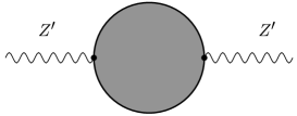
Figure 2: One-particle-irreducible correction to $Z^{\prime}\to Z^{\prime}$.

The partial width corresponding to $Z^{\prime}$ decay into a fermionic pair $f\bar{f}$ can be written in the following form:

$$\Gamma_{Z^{\prime}\to\bar{f}f}=a_{f}^{2}\Gamma_{a_{f}^{2}}+a_{f}v_{f}\Gamma_{a_{f}v_{f}}+v_{f}^{2}\Gamma_{v_{f}^{2}}.$$ (14)

The factors $\Gamma_{a_{f}^{2}}$, $\Gamma_{a_{f}v_{f}}$, and $\Gamma_{v_{f}^{2}}$ are proportional to $m_{Z^{\prime}}$.

IV Estimation Scheme

The main $Z^{\prime}$ decay channels considered by ATLAS and CMS are dielectronic and dimuonic channels. The couplings that enter the corresponding cross sections are $a$, $v_{u}$, and $v_{e}$ for the $pp\to Z^{\prime}\to e^{+}e^{-}$ case and $a$, $v_{u}$, and $v_{\mu}$ for the $pp\to Z^{\prime}\to\mu^{+}\mu^{-}$ case.

Since $v_{\mu}$ was not constrained by the LEP data, we are going to study only the dielectron final state (also note that both these processes are similar at high energies). This allows us to estimate how the LHC data limits the $Z^{\prime}$ couplings compared to the LEP results.

Let us present our estimation scheme. Since there is a maximum-likelihood value for $a^{2}$ from LEP, $a_{\mathrm{ML}}^{2}/m_{Z^{\prime}}^{2}=1.97\times 10^{-2}\mathrm{~{}TeV}^{-2}$, we can consider it as our “optimistic” estimate. There is a “pessimistic” estimate with $a^{2}=0$ for weakly-coupled $Z^{\prime}$. To obtain a kind of an arbitrary estimate, we also consider $a^{2}=a_{\mathrm{ML}}^{2}/4$. Replacing the axial-vector coupling by these three estimates in the $pp\to Z^{\prime}\to e^{+}e^{-}$ cross section, we can investigate possible $v_{e}$ and $v_{u}$ values taking onto account the LHC results on direct searches for $Z^{\prime}$ resonances ATLAS:2013NW ; CMS:2013NW .

First, we need to determine the region of couplings in which the NWA is applicable. The criterion is $\Gamma_{Z^{\prime}}^{2}/m_{Z^{\prime}}^{2}\ll 1$. We set it to

$$\Gamma_{Z^{\prime}}^{2}/m_{Z^{\prime}}^{2}\leq 0.01$$ (15)

To obtain the widest possible region for $v_{e}$ and $v_{u}$, we set the rest of vector couplings to the values at which the corresponding partial widths are minimal. From Eq. (14) and taking into account relations (4), (6) those values are:

$$v_{f}=-\frac{a\Gamma_{av_{f}}}{2\Gamma_{v_{f}^{2}}}\approx\pm 1\times a,\quad f\neq e^{-},u,$$ (16)

where the plus sign is for leptonic couplings, and the minus sign is for quark couplings.

Our next step is to investigate how the currently available LHC data constrains the values of $v_{e}$ and $v_{u}$. Both the ATLAS ATLAS:2013NW and CMS CMS:2013NW results indicate that the lower bounds for the $Z^{\prime}$ mass lie between 2 TeV and 3 TeV. Therefore, we shall derive our constraints for those two values. The $pp\to Z^{\prime}\to e^{+}e^{-}$ cross section is calculated as

$$\sigma_{NWA}=\sigma_{pp\to Z^{\prime}}\times BR(Z^{\prime}\to e^{+}e^{-})=\sigma_{pp\to Z^{\prime}}\times\frac{\Gamma_{Z^{\prime}\to e^{+}e^{-}}}{\Gamma_{Z^{\prime}}}.$$ (17)

We compare this cross section to the experimental upper bounds presented in Refs. ATLAS:2013NW and CMS:2013NW for $pp$ collisions at $\sqrt{S}=8$ TeV. At the considered $Z^{\prime}$ mass values it is always possible to choose such $v_{f}$ ($f\neq e^{-},u$) values, that correspond to the upper bound of the $Z^{\prime}$ decay width in Eq. (15). Therefore, both for $m_{Z^{\prime}}=2$ TeV and $m_{Z^{\prime}}=3$ TeV we set $\Gamma_{Z^{\prime}}$ to $0.1\times m_{Z^{\prime}}$. This will allow us to obtain widest possible LHC-driven intervals for $v_{e}$ and $v_{u}$.

V Results and Discussion

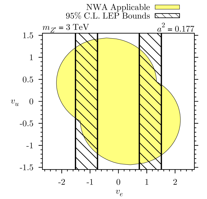
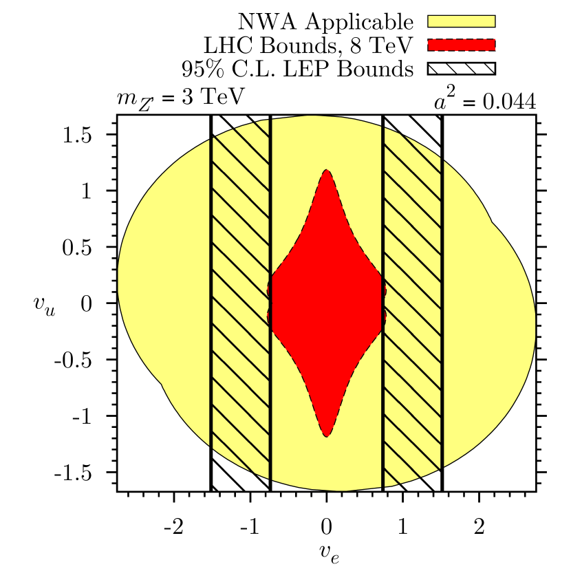
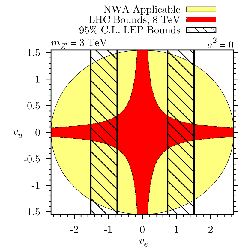
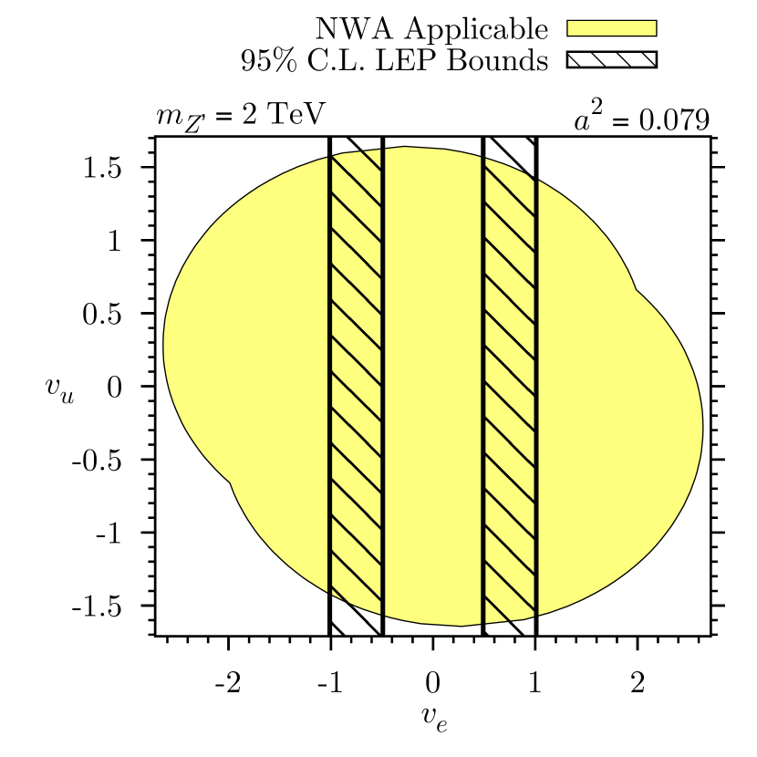
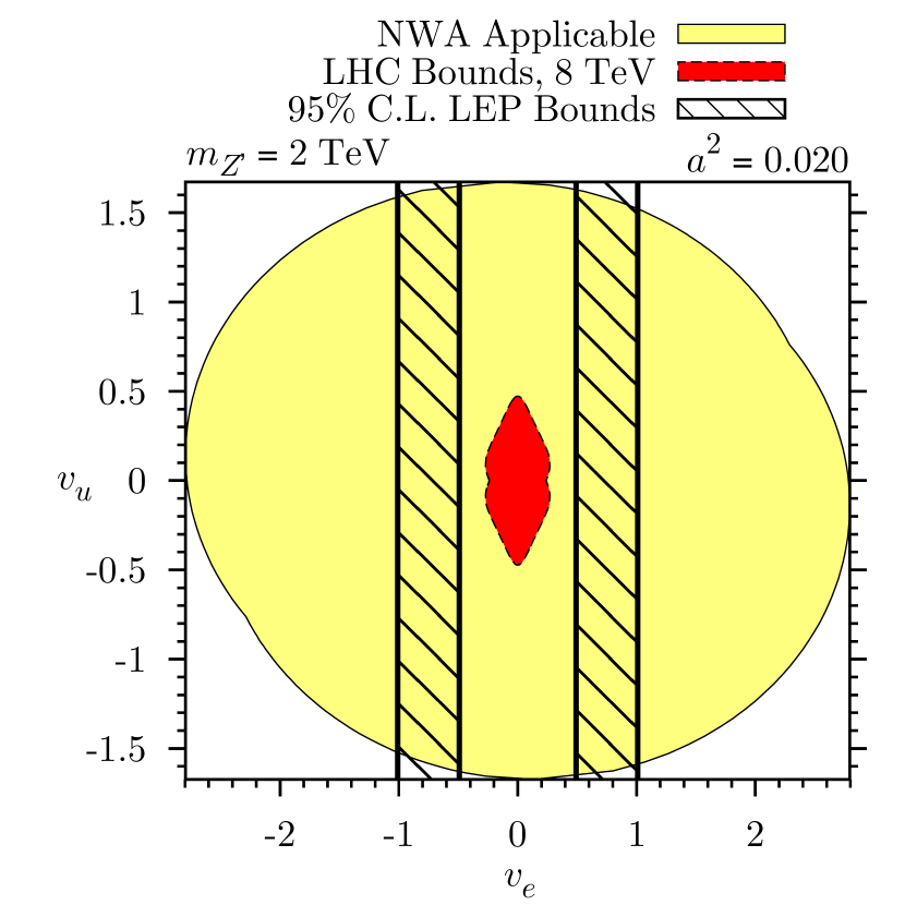
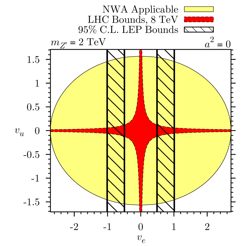
Figure 3: The $v_{u}$-vs-$v_{e}$ planes. First row: $m_{Z^{\prime}}=3$ TeV; second row: $m_{Z^{\prime}}=2$ TeV. The first column is for the “optimistic” estimation scheme, the second column is for the intermediate estimation, and on the plots of the third column the “pessimistic” scheme is presented. The light-gray (yellow) areas represent the coupling values for which the narrow-width approximation is applicable (i.e. $\Gamma_{Z^{\prime}}/m_{Z^{\prime}}\leq 0.1$). The hatched areas are for the 95% CL bounds on the $v_{e}$ coupling (from LEP II data). The dark-gray (red) area represents the $v_{u}$ and $v_{e}$ values allowed by the LHC.

The constraints are shown in Fig. 3 on the $v_{u}$-vs-$v_{e}$ planes. We present the areas of $v_{u}$ and $v_{e}$ values for which the NWA is applicable. For the “optimistic” estimation we use two possible values for the axial-vector coupling: $a/m_{Z^{\prime}}\simeq\pm 0.14\mathrm{~{}TeV}^{-1}$. Also the LEP bounds for $v_{e}$ are shown for comparison.

The ATLAS collaboration ATLAS:2013NW reports upper bounds for $\sigma_{pp\to Z^{\prime}\to e^{+}e^{-}}$ at $1.5\times 10^{-3}$ pb for $m_{Z^{\prime}}=2$ TeV and $2.5\times 10^{-3}$ pb for $m_{Z^{\prime}}=3$ TeV. The “optimistic” estimation for $\sigma_{NWA}$ lies higher than these values, therefore, the LEP maximum-likelihood value $a_{\mathrm{ML}}^{2}/m_{Z^{\prime}}^{2}=1.97\times 10^{-2}\mathrm{~{}TeV}^{-2}$ is discouraged by the LHC results for $m_{Z^{\prime}}$ from 2 TeV to 3 TeV. The LEP maximum-likelihood value is consistent with the LHC results for $Z^{\prime}$ masses below 700 GeV. The region for the “pessimistic” and “intermediate” estimations overlaps with the LHC values, therefore allowing for non-zero upper bounds for the vector couplings. The regions of those are also plotted in Fig. 3. This indicates that the maximum-likelihood LEP value $a_{\mathrm{ML}}^{2}$ is disfavored approximately by one order of magnitude. These two estimates represent a $Z^{\prime}$ with small coupling to the axial-vector currents.

From the plots for the presented estimation schemes we can see that the LHC may limit the vector couplings to $v_{u}^{2}/m_{Z^{\prime}}^{2}\leq 10^{-2}..10^{-3}~{}\mathrm{TeV}^{-2}$, $v_{e}^{2}/m_{Z^{\prime}}^{2}\leq 10^{-1}..10^{-2}~{}\mathrm{TeV}^{-2}$, which is one order lower than the LEP limits. In the considered $Z^{\prime}$ mass region these values are larger than the respective couplings of the SM $Z$ boson ($10^{-3}$ for $v_{e}^{\mathrm{SM}}$ and $2\times 10^{-2}$ for $v_{u}^{\mathrm{SM}}$), but at low energies the $Z^{\prime}$ interactions are strongly suppressed by $1/m_{Z^{\prime}}$. Also it has to be noted, that the renormalization-group relations (4) used in this paper are not applicable for the standard-model $Z$ boson because of different group structure.

It is interesting to calculate the $Z$–$Z^{\prime}$ mixing angle value based on our estimations. Current LEP-driven upper limits for $\theta_{0}$ in different $Z^{\prime}$ models are of order of $10^{-3}$ (see Table IV in Ref. Lang08 ). For our “optimistic” estimate Eq. (5) gives $1.6\times 10^{-3}$ for the $\theta_{0}$ value considering $m_{Z^{\prime}}=2$ TeV. As it was noted, this value is all but ruled out by the LHC data, so for Ableian $Z^{\prime}$ models one may expect $\theta_{0}$ less than (a few)$\times 10^{-4}$.

To obtain more strict bounds, one has to take into account the contributions from the remaining fermions and consider the differential cross-section, rather than working in the narrow-width approximation. Nevertheless, the two presented estimates, being rough, still allow to see, how far it is possible to advance both the direct and indirect $Z^{\prime}$ searches compared to the LEP results.

References

- (1) A. Leike, Phys. Rep. 317, 143 (1999).
- (2) P. Langacker, Rev. Mod. Phys. 81, 1199-1228 (2008).
- (3) T. Rizzo, Phenomenology and the LHC, in Colliders and neutrinos: The window into physics beyond the standard model; Proc of Summer School TASI 2006, Boulder, USA, June 4-30, 2006, eds. S. Dawson and R.N. Mohapatra, p.537-575, e-print hep-ph/0610104.
- (4) N. Hod (on behalf of the ATLAS collaboration), Search for heavy resonances, and resonant diboson production with the ATLAS detector, Proceedings of Hadron Collider Physics Symposium 2012 (HCP 2012), Kyoto, Japan, November 12-16, 2012, eds. M. Ishino, K. Nagano, S. Asai, EPJ Web Conf. 49, 15004 (2013), e-print arXiv:1303.4287 [hep-ex]
- (5) CMS Collaboration, Phys. Lett. B 720, 63 (2013) e-print arXiv:1212.6175 [hep-ex].
- (6) E. Boos, V. Bunichev, L. Dudko and M. Perfilov, Phys. Lett. B 655, 245 (2007)
- (7) E.E. Boos, M.A. Perfilov, M.N. Smolyakov and I.P. Volobuev, Theor.Math.Phys. 170, 90-96 (2012)
- (8) P. Osland, A. A. Pankov, N. Paver and A. V. Tsytrinov Phys. Rev. D 79, 115021 (2009).
- (9) A. Gulov and A. Kozhushko, e-print arXiv:1209.5022 [hep-ph].
- (10) J. Erler, P. Langacker, S. Munir and E. R. Pena, JHEP 08, 017 (2009).
- (11) F. del Aguila, J. de Blas and M. Perez-Victoria, JHEP 1009, 033 (2010), e-print arXiv:1005.3998
- (12) J. Erler, P. Langacker, S. Munir and E. Rojas, e-print arXiv:1010.3097v1 [hep-ph].
- (13) G. Corcella, EPJ Web Conf. 60, 18011 (2013), e-print arXiv:1307.1040 [hep-ph]
- (14) V. V. Andreev, G. Moortgat-Pick, P. Osland, A. A. Pankov and N. Paver, e-print arXiv:1205.0866 [hep-ph]
- (15) V. V. Andreev, G. Moortgat-Pick, P. Osland, A. A. Pankov and N. Paver, Eur. Phys. J. C 72, 2147 (2012), e-print arXiv:1205.0866 [hep-ph]
- (16) Q.-H. Cao, Z. Li, J.-H. Yu and C.-P. Yuan, Phys. Rev. D 86, 095010 (2012).
- (17) L. Basso, K. Mimasu and S. Moretti, JHEP 1211, 060 (2012).
- (18) E. Accomando, D. Becciolini, A. Belyaev, S. Moretti and C. Shepherd-Themistocleous, JHEP 10, 153 (2013), e-print arXiv:1304.6700 [hep-ph]
- (19) O.J.P. Eboli, J. Gonzalez-Fraile and M.C. Gonzalez-Garcia, Phys. Rev. D 85, 055019 (2012).
- (20) A. V. Gulov and V. V. Skalozub, Eur. Phys. J. C 17, 685 (2000).
- (21) A. V. Gulov and V. V. Skalozub, Phys. Rev. D 61, 055007 (2000).
- (22) A. V. Gulov and V. V. Skalozub, e-print arXiv:0905.2596v2 [hep-ph].
- (23) A. V. Gulov and V. V. Skalozub, Int. J. Mod. Phys. A 25, 5787-5815 (2010).
- (24) A. V. Gulov and A. A. Kozhushko, Int. J. Mod. Phys. A 26, 4083-4100 (2011).
- (25) A.D. Martin, W.J. Stirling, R.S. Thorne and G. Watt, Eur. Phys. J. C 63, 189 (2009); ibid. 64, 653 (2009) http://projects.hepforge.org/mstwpdf/.
- (26) R. Gavin, Y. Li, F. Petriello and S. Quackenbush, Comput. Phys. Commun. 182, 2388-2403 (2011) http://gate.hep.anl.gov/fpetriello/FEWZ.html.
- (27) T. Hahn, Comput. Phys. Commun. 140, 418 (2001); http://www.feynarts.de/.
- (28) T. Hahn and M. Perez-Victoria, Comput. Phys. Commun. 118, 153 (1999); http://www.feynarts.de/formcalc/, http://www.feynarts.de/looptools/.