Reduced variable optimization methods via implicit functional dependence with applications

Abstract

Optimization methods have been broadly applied to two classes of objects viz. (i) modeling and description of data and (ii) the determination of the stationary points of functions. The overwhelming majority of these methods treat explicitly the variables relevant to the function optimization, where these parameters are independently varied with a weightage factor. Here, a theoretical basis is developed which suggests algorithms that optimizes an arbitrary number of variables for classes (i) and (ii) by the minimization of a function of a single variable deemed the most significant on physical or experimental grounds form which all other variables can be derived. Often, one or more key variables play a physically more significant role than others even if all the variables are equally weighted so that these key optimized variables serve as criteria whether or not reasonable solutions have been obtained, independently of the other variables. Algorithms that focus on a reduced variable set also avoid problems associated with multiple minima and maxima that arise because of the large numbers of parameters, and could increase the accuracy of the determination by cutting down on machine errors. The methods described could have potentially significant applications in the physical sciences where the optimization of one physically significant variable has priority over the other variables as in the energy-position optimization schemes of computational quantum mechanics applied to structure determination, and in chemical kinetics trajectory calculations where the trajectory variable is linked to many other variables of secondary importance. For (i), we develop both an approximate but computationally more tractable method and an exact method where the single controlling variable $k$ of all the other variables $\mathbf{P}(k)$ passes through the local stationary point of the least squares (LS) metric. For (ii), an exact theory is developed whereby the optimized function of an independent variation of all parameters coincides with that due to single parameter optimization. The implicit function theorem has to be further qualified to arrive at this result. The topology of the surfaces of constant value of the target or cost function are considered for all the methods. A real world application of the above implicit methodology to rate constant and final concentration parameter determination for first and second order chemical reactions from published data is attempted to illustrate its utility. This work is different from and more general than all the reduction schemes for conditional linear parameters used for example in extracting data from mixed signal spectra of physical quantities such as found in laser spectroscopy since it is valid for conditional and nonconditional nonlinear parameters. Nor is it a subset of the Adomian decomposition method (ADM) used for estimating solutions of differential equations, which still require boundary conditions that do not feature in topics (i) and (ii).

MSC code 41-04   41A28   41A58   41A63   41A65

PACS code 05.10.-a  07.05.Bx   02.60.Pn   02.60.Cb   82.20.Nk

1 Introduction

The following theory and elaboration revolve about properties of constrained and unconstrained functions that are continuous and differentiable to various specified degrees[1, 2], and the existence of implicit functions [3] and the form of the function to be optimized. The implicit function theorem is applied in a way that requires further qualified because the optimization problem is of an unconstrained kind without any redundant variables. Methods (i)a,b (Secs.(2 ) and (3) respectively) refers to modeling of data [4, Chap.15,p.773-806] where the form of the function $Q_{MD}(\mathbf{P},k)$ with independently varying variables $(\mathbf{P},k)$ have the general form

$$Q_{MD}(\mathbf{P},k)=\sum_{i=1}^{N_{c}}(y_{i}-f(\mathbf{P},t_{i},k))^{2}$$ (1)

where $y_{i}$ and $t_{i}$ are datapoints and $f$ a known function, and optimizations of $Q_{MD}$ may be termed a least squares (LS) fit over parameters $(\mathbf{P},k)$ which are independently optimized. Method (ii) focuses on optimizing a general $Q_{Opt}(\mathbf{P},k)$ function, not necessarily LS in form. There are many standard and hybrid methods to deal with such optimization [4, Ch.10], such as golden section searches in 1-D, simplex methods over multidimensions [4, p.499-525], steepest descent and conjugate methods [5] and variable metric methods in multidimensions [4, p.521-525] . Hybrid methods include multidimensional (DFP) secant methods [6], BFGS (secant optimization) [7] and RFO (rational function optimization) [8] which is a Newton-Raphson technique utilizing a rational function rather than a quadratic model for the function close to the solution point. Global deterministic optimization schemes combine several of the above approaches [9, sec 6.7.6] Other ad hoc, physical methods perhaps less easy to justify analytically include probabilistic "basin-hopping" algorithms [9, sec 6.7.4], simulated annealing methods [10] and genetic algorithms [9, p.346]. An analytical justification on the other hand is attempted here, but in real-world problems some of the assumptions (e.g. $\mathcal{C}^{2}$ continuity, compactness of spaces) may not always obtain. For what follows, the distance metric used are all Euclidean, represented by $|\cdot|$ or $\|\cdot\|$ where $det\,\|\cdot\|$ represents the determinant of the matrix $|\cdot\|$. Reduction of the number of variables to be optimized is possible in the standard matrix regression model only if conditional linear parameters $\boldsymbol{\beta}$ exists [11], where these $\boldsymbol{\beta}$ variables do not appear in the final $S(\boldsymbol{\theta})$ expression of the least squares function (2) to be optimized, whereas the $\boldsymbol{\phi}$ nonconditional linear parameters do and are a subset of the $\boldsymbol{\theta}$ variables; for the existence of each conditional linear parameter, there is a unit reduction in the number of independent parameters to be optimized. These reductions in variable number occurs for any "expectation function" $f(\mathbf{x},\boldsymbol{\theta})$ which is the model or law for which a fitting is required, where there are $N$ different datapoints $\mathbf{x_{i}},\,i=1,2,\ldots N$ that must be used to determine the $p$ parameter variables $\boldsymbol{\theta}$ [11, p.32,Ch.2]. A conditionally linear parameter $\theta_{i}$ exists if and only if the derivative of the expectation function $f(\mathbf{x},\boldsymbol{\theta})$ with respect to $\theta_{i}$ does not involve - in other words is independent of - $\theta_{i}$. Clearly such a condition may severely limit the number of parameters that can be neglected for the expectation function variables when the prescribed matrix regressional techniques are employed [11, Sec.3.5.5, p.85] where the residual sum of squares is minimized:

$$S(\boldsymbol{\theta})=\left\|\mathbf{y}-\boldsymbol{\eta}(\boldsymbol{\theta})\right\|^{2}.$$ (2)

The $N$-vectors $\boldsymbol{\eta(\theta)}$ in $P$ dimensional space defines the expectation surface. If the $\boldsymbol{\theta}$ variables are partitioned into the conditional linear parameters $\boldsymbol{\beta}$ and the other nonlinear parameters $\boldsymbol{\phi}$, then the response can be written $\boldsymbol{\eta(\beta,\phi)=A(\phi)\beta}$. Golub and Pereyra [12] used standard Gauss-Newton algorithm to minimise $S_{2}(\boldsymbol{\phi})=\left\|\mathbf{y}-\boldsymbol{A(\phi)}\boldsymbol{\hat{\beta}(\phi)}\right\|^{2}$ that depended only on the nonlinear parameters $\boldsymbol{\phi}$ where $\boldsymbol{\hat{\beta}(\phi)}=\boldsymbol{A^{+}(\phi)}\boldsymbol{y}$ with $\boldsymbol{A^{+}}$ being a defined pseudoinverse of $\boldsymbol{A}$ [11, Sec.3.5.5,p.85] where $\boldsymbol{A^{+}}$ and $\boldsymbol{A}$ are matrices. The variables must be separable as discussed above and the number of variable reduction is only equal to the number of conditional linear parameters that exists for the problem. In applications, the preferred algorithm that exploits this valuable variable reduction is called Variable Projection. There are many applications in time resolved spectroscopy that is heavily dependent on this technique and many references to the method are given in the review by van Stokkum et al. [13]. Recently this method of variable projection has been extended in a restricted sense [14] in the field of inverse problems, which is not related to our method of either modeling or optimization, nor is the methodology related to the implicit function methods. In short, much of the reported methods developed are $ad\,hoc$, meaning that they are constructed to face the specific problems at hand with no pretense to any all-encompassing generality and this work too is $ad\,hoc$ in the sense of suggesting variable reduction with specific classes of non-inverse problems as indicated where the work develops a method of reducing the variable number to unity for all variables in the expectation function space irrespective of whether they are conditional or not by approximating their values by a method of averages (for method(i)a) without any form of linear regression being used in determining their approximations during the minimization cycles, and without necessarily using the standard matrix theory that is valid for a very limited class of functions. Methods (i)b and (ii) are exact treatments. No "‘eliminating"’ of conditional linear parameters are involved in this nonlinear regression method because they are explicitly calculated. Nor is any projection in the mathematical sense involved. These more general methods could have useful applications in deterministic systems comprising many parameters that are all linked to one variable, the primary one (denoted $k$ here) that is considered on physical grounds to be the most important one. A generalization of this method would be to select a smaller set of variables than the full parameter list. Examples of multiparameter complex systems include those for multiple-step elementary reactions each with its own rate constant that gives rise to photochemical spectra signals that must be resolved unambiguously [15]. All these complex and coupled processes in physical theories are related by postulated laws $Y_{law}(\mathbf{P},k,t)$ that feature parameters $(\mathbf{P},k)$. Other examples include quantum chemical calculations with many topological and orientation variables that need to be optimized with respect to the energy, but in relation to one or a few variables, such as the molecular trajectory parameter during a chemical reaction where this variable is of primary significance in deciding on the ’reasonableness’ of the analysis [9, Sec. 6.2.3,p.294]. Method (i)a and (i)b below refer to LS data-fitting algorithms. Method (i)a is an approximate method where it is proved under certain conditions that it could be a more accurate determination of parameters compared to a standard LS fit using (1). Method (i)b develops the methodology whereby its optimum value for $Q_{MD}$ with domain values $(\mathbf{P},k)$ coincides with that of the standard LS method where the $(\mathbf{P},k)$ variables are varied independently. Also discussed are the relative accuracy of both methods (i)a in subsection (2.2)and (i)b (endnote at end of section 3). Method (ii) develops a single parameter optimization where the conditions of an arbitrary $Q_{OPT}(\mathbf{P},k)$ function are met simultaneously, viz.

$$\frac{\partial Q_{OPT}(k)}{\partial k}=0\rightarrow\left\{\frac{\partial Q_{OPT}(\mathbf{P},k)}{\partial\mathbf{P}}=0,\frac{\partial Q_{OPT}(\mathbf{P},k)}{\partial k}=0\right\}.$$

We note that methods (i)a, (i)b and (ii) are not related to the Adomian decomposition method and its variants that expands polynomial coefficients [16] for solutions to differential equations not connected to estimation theory; indeed here there are no boundary values that determine the solution of the differential equations.

2 Method (i)a theory

Deterministic laws of nature are sometimes written - for the simplest examples- in the form

$$Y_{law}=Y_{law}(\mathbf{P},k,t)$$ (3)

linking the variable $Y_{law}$ to $t$. The components of $\mathbf{P}$, $P_{i}(i=1,2,...N_{p})$ and $k$ are parameters. Verification of a law of form (3) relies on an experimental dataset $\{(Y_{exp}(t_{i}),\,t_{i}),i=1,2,...N)\}$. The $t$ variable could be a vector of variable components of experimentally measured values or a single parameter as in the example below where $t_{i}$ denotes values of time $t$ in the domain space. The vector form will be denoted $\mathbf{x}$. Variables $(\mathbf{x})$ are defined as members of the ’domain space’ of the measurable system and similarly $Y_{law}$ is the defined range or ’response’ space of the physical measurement. Confirmation or verification of the law is based on (a) deriving experimentally meaningful values for the parameters $(\mathbf{P},k)$ and (b) showing a good enough degree of fit between the experimental set $Y_{exp}(t_{i})$ and $Y_{law}(t_{i})$. In real world applications, to chemical kinetics for instance, several methods [17, 18, 19, 20, etc.] have been devised to determine the optimal $\mathbf{P},k$ parameters, but most if not all these methods consider the aforementioned parameters as autonomous and independent (e.g. [18]). A similar scenario broadly holds for current state of the art applications of structural elucidation via energy functions [9]. To preserve the viewpoint of the inter-relationship between these parameters and the experimental data, we devise a scheme that relates $\mathbf{P}$ to $k$ for all $P_{i}$ via the set $\{Y_{exp}(t_{i}),t_{i}\}$, and optimize the fit over $k$-space only. i.e. there is induced a $P_{i}(k)$ dependency on $k$ via the the experimental set $\{Y_{exp}(t_{i}),t_{i}\}$. The conditions that allow for this will also be stated.

2.1 Details of method (i)a

Let $N^{\prime}$ be the number of dataset pairs $\{Y_{exp}(t_{i}),t_{i}\}$, $N_{p}$ the number of components of the $\mathbf{P}$ parameter, and $N_{s}$ the number of singularities where the use of a particular dataset $(Y_{exp},t)$ leads to a singularity in the determination of $\bar{P}_{i}(k)$ as defined below and which must be excluded from being used in the determination of $\bar{P}_{i}(k)$. Then $(N_{p}+1)\leq(N-N_{s})$ for the unique determination of $\{\mathbf{P},k\}$. Let $N_{c}$ be the total number of different datasets that can be chosen which does not lead to singularities. If the singularities are not choice dependent, i.e. a particular data-set pair leads to singularities for all possible choices, then we have the following definition for $N_{c}$ where ${}^{N-N_{s}}C_{N_{p}}=N_{c}$ is the total number of combinations of the data-sets $\{Y_{exp}(t_{i}),t_{i}\}$ taken $N_{p}$ at a time that does not lead to singularities in $P_{i}$. In general, $N_{c}$ is determined by the nature of the data sets and the way in which the proposed equations are to be solved. Write $Y_{law}$ in the form

$$Y_{law}(t,k)=f(\mathbf{P},t,k)$$ (4)

and for a particular dataset $\{Y_{exp}(t_{i}),t_{i}\}$, write $f(i)\equiv f(\mathbf{P},t_{i},k)$. Define the vector function $\mathbf{f_{g}}$ with components $f_{g}(i)\equiv Y_{exp}(t_{i})-f(i)=f_{g}(i)(\mathbf{P},k)$. Assume $\mathbf{f_{g}}\in\mathcal{C}^{1}$ defined on an open set $K_{0}$ that contains $k_{0}$.

Lemma 1.

For any such $k_{0}$ if $det\left\|\frac{\partial f_{g}(i)(\mathbf{P},k_{0})}{\partial P_{j}}\right\|\neq 0$, $\exists$ the unique function $\mathbf{P}(k)\in\mathcal{C}^{1}$ (with components $P_{i}(k)\ldots P_{N_{c}}(k)$) defined on $K_{0}$ where $\mathbf{P}(k_{0})=\mathbf{P_{0}}$, and where $\mathbf{f_{g}}(\mathbf{P}(k),k)=0$ for every $k\in K_{0}$.

Proof.

The above follows from the Implicit function theorem (IFT) [3, Th.13.7,p.374] where $k\in K_{0}$ is the independent variable for the existence of the $\mathbf{P}(k)$ function. ∎

We seek the solutions for $\mathbf{P}(k)$ subject to the above conditions for our defined functions. Map $f\longrightarrow Y_{th}(\bar{\mathbf{P}},t,k)$ as follows

$$Y_{th}(t,k)=f(\bar{\mathbf{P}},t,k)$$ (5)

where the term $\bar{\mathbf{P}}$ and its components are defined below and where $k$ is a varying parameter. For any of the $(i_{1},i_{2},\ldots,i_{N_{p}})$ combinations denoted by a combination variable $\alpha\equiv(i_{1},i_{2},\ldots,i_{N_{p}})$ where $i_{j}\equiv(Y_{exp}(t_{i_{j}}),t_{i_{j}})$ is a particular dataset pair, it is in principle possible to solve for the components of $\bar{\mathbf{P}}$ in terms of $k$ through the following simultaneous equations:

$$\begin{array}[]{rll}Y_{exp}(t_{i_{1}})&=&f(\mathbf{P},t_{i_{1}},k)\\[14.22636pt] Y_{exp}(t_{i_{2}})&=&f(\mathbf{P},t_{i_{2}},k)\\ &\vdots&\\ Y_{exp}(t_{i_{N_{p}}})&=&f(\mathbf{P},t_{i_{N_{p}}},k)\end{array}$$ (6)

from Lemma 1. And each $\alpha$ choice yields a unique solution $P_{i}(k,\alpha)\,(i=1,2\ldots N_{p})$ where $P_{i}(k,\alpha)\in\mathcal{C}^{1}$. Hence any functions of $P_{i}(k,\alpha)$ involving addition and multiplication are also in $\mathcal{C}^{1}$. For each $P_{i}$, there will be $N_{c}$ different solutions, $P_{i}(k,1),P_{i}(k,2),\ldots P_{i}(k,N_{c})$ . We can define an arithmetic mean (there are several possible mean definitions that can be utilized) for the components of $\bar{\mathbf{P}}$ as

$$\bar{P_{i}}(k)=\frac{1}{N_{c}}\sum_{j=1}^{N_{c}}P_{i}(k,j).$$ (7)

In choosing an appropriate functional form for $\bar{\mathbf{P}}$ (eq.7) we assumed equal weightage for each of the dataset combinations; however the choice is open, based on appropriate physical criteria. We verify below that the choice of $\bar{\mathbf{P}}(k)$ satisfy the constrained variation of the LS method so as to emphasize the connection between the level-surfaces of the unconstrained LS with the line function $\bar{\mathbf{P}}(k)$ .

Figure 1: Depiction of how the $k$ variation optimizing $Q$ leads to a solution on a level surface of the $Q_{T}$ function where $Q_{T}\leq Q$.

Each $P_{i}(k,j)$ is a function of $k$ whose derivative is known either analytically or by numerical differentiation. To derive an optimized set, then for the LS method, define

$$Q(k)=\sum_{i=1^{\prime}}^{N^{\prime}}(Y_{exp}(t_{i})-Y_{th}(k,t_{i}))^{2}.$$ (8)

Then for an optimized $k$, we have $Q^{\prime}(k)=0.$ Defining

$$R(k)=\sum_{i=1^{\prime}}^{N^{\prime}}(Y_{exp}(t_{i})-Y_{th}(k,t_{i})).Y_{th}^{\prime}(k,t_{i})$$ (9)

the optimized solution of $k$ corresponds to $R(k)=0$ which has been reduced to a one dimensional problem. The standard LS variation on the other hand states that the variables $P_{T}=\{\mathbf{P},k\}$ in (4) are independently varied so that

$$Q_{T}(P_{T})=\sum_{i=1}^{N^{\prime}}(Y_{exp}(t_{i})-f(P_{T},,t_{i}))^{2}.$$ (10)

with solutions for $Q_{T}$ in terms of $P_{T}$ whenever $\partial Q_{T}/\partial P_{T}=0$. Of interest is the relationship between the single variable variation in (8 ) and the total variation in (10). Since $\overline{\mathbf{P}}$ is a function of $k$, then (10) is a constrained variation where

$$\delta Q(k)=\delta Q(\overline{\mathbf{P}},k)=\left(\frac{\partial Q}{\partial\overline{\mathbf{P}}}.\delta\overline{\mathbf{P}}+\frac{\partial Q}{\partial k}\right)$$ (11)

subjected to $g_{i}(\overline{\mathbf{P}},k)=\bar{P}_{i}-h_{i}(k)=0$ (i.e. $\bar{P}_{i}=h_{i}(k)$ for some function of k) and where $\bar{P}_{i}$ are the components of $\bar{\mathbf{P}}$. According to the Lagrange multiplier theory [3, Th.13.12,p.381] the function $f:\mathbb{R}^{n}\rightarrow\mathbb{R}$ has an optimal value at $x_{0}$ subject to the constraints $g:\mathbb{R}^{n}\rightarrow\mathbb{R}^{m}$ over the subset $S$ where $\mathbf{g}=(g_{1},g_{2}\ldots g_{m})$ vanishes, i.e. $x_{0}\in X_{0}$ where $X_{0}=\{x:x\in S,\mathbf{g}(x)=0\}$ when either of the following equivalent equations (12,13) are satisfied

$$D_{r}f(x_{o}) + \sum_{k=1}^{m}\lambda_{k}D_{r}g_{k}(x_{0})=0\,\,(r=1,2,\ldots n)$$ (12)

$$\nabla f(x_{0}) + \lambda_{1}\nabla g_{1}(x_{0})+\ldots\lambda_{m}\nabla g_{m}(x_{0})=0$$ (13)

where $det\|D_{j}g_{i}(x_{0})\|\neq 0$ and the $\lambda$’s are invariant real numbers. We refer to $\bar{P}_{i}$ as any variable that is a function of $k$ constructed on physical or mathematical grounds, and not just to the special defined in (7). Write

$$g_{i}=\bar{P}_{i}-p_{i}(k)=0\,(i=1,2,\ldots N_{p})$$ (14)

where $D_{j}g_{i}(x_{o})=\delta_{ij}$ since $D_{j}=\partial/\partial\bar{P}_{j}$ and therefore $det\|D_{j}g_{i}\neq 0\|$. We abbreviate the functions $f(i)=f(\mathbf{P},t_{i},k)$ and $\bar{f}(i)=f(\mathbf{\bar{P}},t_{i},k)$. Define

$$f_{Q}(x)\equiv Q(\bar{\mathbf{P}},k,t)=\sum_{i=1^{\prime}}^{N^{\prime}}(Y_{exp}(t_{i})-\bar{f}(i))^{2}$$ (15)

where $Y_{exp}(t_{i})$ are the experimental subspace variables as in (6) with $x\in X_{0}$ defined above. We next verify the relation between $Q(k)$ and $Q_{T}$ .

Verification 2.

The solution $Q^{\prime}(k)$=R(k)=0 of (9 ) is equivalent to the variation of $f_{Q}(x)$ defined in (15) subjected to constraints $g_{i}$ of (14).

Proof.

Define the Lagrangian to the problem as $\mathcal{L}=f_{Q}(x)+\sum_{i=1}^{N_{p}}\lambda_{i}g_{i}$. Then the equations that satisfy the stationary condition

$$\frac{\partial\mathcal{L}}{\partial\bar{P}_{j}}=0\,\,(j=1,2,\ldots N_{p});\frac{\partial\mathcal{L}}{\partial k}=0$$ (16)

reduces to the (equivalent) simultaneous equations

$$\sum_{i=1}^{N^{\prime}}(Y_{exp}(t_{i}) - \bar{f}(i))\frac{\partial\bar{f}(i)}{\partial\bar{P}_{j}}=\lambda^{\prime}_{j}\,\,(j=1,2,\ldots N_{p})$$ (17)

$$\sum_{i=1}^{N^{\prime}}(Y_{exp}(t_{i}) - \bar{f}(i))\frac{\partial\bar{f}(i)}{\partial k}+\sum_{j=1}^{N_{p}}\lambda^{\prime}_{j}\frac{\partial p_{j}}{\partial k}=0$$ (18)

Substituting $\lambda^{\prime}_{j}$ in (17) to (18) leads to

$$\sum_{i=1}^{N^{\prime}}(Y_{exp}(t_{i})-\bar{f}(i))\frac{\partial\bar{f}(i)}{\partial k}+\sum_{j=1}^{N_{p}}\sum_{i=1}^{N^{\prime}}(Y_{exp}(t_{i})-\bar{f}(i)).\frac{\partial\bar{f}(i)}{\partial\bar{P}_{j}}.\frac{\partial p_{j}}{\partial k}=0.$$ (19)

Since $\frac{d\bar{P}_{i}}{dk}=\frac{\partial\bar{p}_{i}}{\partial k}$, then (19) is equal to $\frac{dQ(\bar{\mathbf{P}},k,t)}{dk}=0$ of the $Q$ functions in (10,11 and 15). ∎

Of interest is the theoretical relationship of the $\bar{\mathbf{P}},k$ variables of the $Q$ function described by (11,8) denoted $Q_{1}$ and those of the free variational $Q$ function of (15) denoted $Q_{2}$ with the variable set which can be written

$$Q_{1} = Q(\bar{\mathbf{P}},t,k)$$ (20)

$$Q_{2} = Q(\mathbf{P},t,k)$$ (21)

which is given by the following theorem, where we abbreviate $\alpha_{i}=(Y_{exp}(t_{i})-f(\mathbf{P},t_{i},k))$ and $\bar{\alpha}_{i}=(Y_{exp}(t_{i})-f(\bar{\mathbf{P}},t_{i},k))$ where we note that the $f$ functional form is unique and of the same form for both these $\alpha$ variables.

Theorem 3.

The unconstrained LS solution to $Q_{2}=Q(\mathbf{P},k,t)$ for the independent variables $\{\mathbf{P},k\}$ is also a solution for the constrained variation single variable $k^{\prime}$ where $\mathbf{P}=\bar{\mathbf{P}}(k^{\prime}),k=k^{\prime}$. Further, the two solutions coincide if and only if

$$\sum_{i=1}^{N^{\prime}}(Y_{exp}(t_{i})-f(\bar{\mathbf{P}},t_{i},k))\frac{\partial f(\bar{\mathbf{P}},t_{i},k)}{\partial\bar{P}_{j}}\,,j=1,2,\ldots N_{p}.$$

Proof.

The $Q_{2}$ unconstrained solution is derived from the equations

$$\frac{\partial Q_{2}}{\partial P_{j}} = c.\sum_{i=1}^{N^{\prime}}\alpha_{i}\frac{\partial f(i)}{\partial P_{j}}=0\,,j=1,2,\ldots N_{p}$$ (22)

$$\frac{\partial Q_{2}}{\partial k} = c.\sum_{i=1}^{N^{\prime}}\alpha_{i}\frac{\partial f(i)}{\partial k}=0$$ (23)

with $c$ being constants. If there is a $\bar{\mathbf{P}}(k)$ dependency, then we have

$$\frac{dQ_{1}(k)}{dk}=c.\sum_{j=1}^{N_{p}}\left(\sum_{i=1}^{N^{\prime}}\bar{\alpha}_{i}\frac{\partial\bar{f}(i)}{\partial P_{j}}\right)\frac{\partial\bar{P}_{j}}{\partial k}+c.\sum_{i=1}^{N^{\prime}}\bar{\alpha}_{i}\frac{\partial\bar{f}(i)}{\partial k}.$$ (24)

If the variable set $\{\mathbf{P},k\}$ satisfies (22) and (23) in unconstrained variation, then the values when substituted into (24 ) satisfies the equation $\frac{dQ_{1}(k)}{dk}=0$ since $f(i)$ and $\bar{f}(i)$ are the same functional form. This proves the first part of the theorem. The second part follows from the converse argument, where from (24 ), if $\frac{dQ_{1}(k)}{dk}=0$, then setting one factor to zero in (2.1 ) leads to the implication of (26)

$$\sum_{i=1}^{N^{\prime}}\bar{\alpha}_{i}\frac{\partial\bar{f}(i)}{\partial\bar{P}_{j}} = 0\,,j=1,2,\ldots N_{p}$$

$$\Rightarrow$$

$$\sum_{i=1}^{N^{\prime}}\bar{\alpha}_{i}\frac{\partial\bar{f}(i)}{\partial k} = 0$$ (26)

the solution set $\{\bar{\mathbf{P}}(k^{\prime}),k^{\prime}\}$ which satisfies $\frac{dQ_{1}(k)}{dk}=0$ is satisfied by the conditions of both (2.1) and (26). Then (2.1) satisfies (22) and (26) satisfies (23). ∎

The theorem, verification and lemma above do not indicate topologically under what conditions a coincidence of solutions for the constrained and unconstrained models exists. Fig.(1) depicts the discussion below. From theorem (3), if set $A$ represents the solution $\{\mathbf{P},k\}$ for the unconstrained LS method and set $B=\{\mathbf{\bar{P}},k^{\prime}\}$ for the constrained method , then $B\supseteq A$. Define $k$ within the range $k_{1}\leq k\leq k_{2}$. Then $k$ is in a compact space, and since $\mathbf{P}(k)\in\mathcal{C}^{1}$,$\mathbf{P}(k)$ is uniformly continuous, [2, TH.8,p.79]. Then admissible solutions to the above constraint problem with the inequality $B\supseteq A$ implies $Q(\mathbf{P}(k))\geq Q_{min}$ where $Q_{min}$ is the unconstrained minimum. The unconstrained $Q=Q_{T}$ LS function to be minimized in (10) implies

$$\nabla Q=0\,\,(\frac{\partial Q}{\partial k}=\frac{\partial Q}{\partial P_{i}}=0\,\mathrm{for}\,i=1,2,\ldots N_{p})$$ (27)

Defining the constrained function $Q_{c}(k)=\sum_{i=1}^{N^{\prime}}(Y_{exp}(i)-f(\mathbf{P}(k),t_{i},k))^{2}$ then $Q_{c}(k)=Q\circ P_{T}$ where $P_{T}=(P_{1}(k),P_{2}(k),\ldots P_{N_{p}}(k),k)^{T}$. Because $Q^{\prime}_{c}(k)=\left(\frac{\partial Q}{\partial\mathbf{P}},\frac{\partial Q}{\partial k}\right)\cdot\left(P_{1}^{\prime}(k)\ldots P_{N_{p}}(k),k\right)^{T}$, solutions occur when (i) $\nabla Q=0$ corresponding to the coincidence of the local minimum of the unconstrained $Q$ for the best choice for the line with coordinates $(\mathbf{P}(k),k)$ as it passes through the local unconstrained minimum and (ii) $P^{\prime}_{i}(k)=0,(i=1,2,\ldots N_{p}),\frac{\partial Q}{\partial k}=0$ where this solution is a special case of (iii) when the vector $P^{\prime}_{T}$ is $\perp$ to $\nabla Q\neq 0$, i.e. $P^{\prime}_{T}$ is at a tangent to the surface $Q=S_{2}$ for some $S_{2}\geq Q_{min}$ where this situation is shown in Fig.(1) where the vector is tangent at some point of the surface $Q_{T}=S_{2}$. Whilst the above characterizes the topology of a solution, the existence of a solution for the line $(\mathbf{P}(k),k)$ which passes through the point of the unconstrained minimum of $Q_{T}$ is proven below under certain conditions where a set of equations are constructed to allow for this exceptionally important application. Also discussed is the case when it may be possible for unconstrained solution set $U$ to satisfy the inequality $Q_{T}(U)\geq Q_{c}$, where $Q_{C}$ is a function designed to accommodate all solutions of (6).

2.2 Discussion of LS fit for a function $Q_{c}$ with a possibility of a smaller LS deviation than for $\{\mathbf{P},k\}$ parameters derived from a free variation of eq.(10)

The LS function metric such as (10) implied $Q(\mathbf{P},k)\leq Q(\mathbf{\bar{P}},k))$ at a stationary (minimum) point for variables $(\mathbf{P},k)$. On the other hand, the sets of solutions (6), $N_{c}$ in number provides for each set exact solutions $\mathbf{P}(k)$ averaged to $\mathbf{\bar{P}}(k)$. If the $\{\mathbf{\bar{P}}_{i}\},i=1,2,\ldots N_{c}$ solutions are in a $\delta$-neighbourhood, then it may be possible that the composite function metric to be optimized over all the sets of equations $\{\}_{i}$, $N_{c}$ in number defined here

$$Q_{c}(\mathbf{P},k)=\sum_{i\in\{\}_{1},\{\}_{2}\ldots\{\}_{N_{c}}}(Y_{exp}-f(i))^{2}$$ (28)

could be such that

$$Q_{c}(\mathbf{P},k)\geq Q_{c}(\mathbf{\bar{P}},k)$$ (29)

implying that, under these conditions, the $Q_{c}$ of (28) is a better measure of fit. For what follows, the $\mathbf{P}(k)_{\{\}_{i}}$ for equation set $\{\}_{i}$ obtains for all $k$ values of the open set $\mathcal{S},\,\,k\in\mathcal{S}$, from the IFT, including $k_{0}$ which minimises (8). Another possibility that will be discussed briefly later is where in (28), all $\{\mathbf{P},k\}$ are free to vary. Here we consider the case of the $N_{c}$ $\mathbf{P}$ values averaged to $\mathbf{\bar{P}}$ for some $k$. We recall the Intermediate-value theorem (IVT) [3, Th.4.38,p.87]for real continuous functions $f$ defined over a connected domain $S$ which is a subset of some $\mathbb{R}^{n}$. We assume that the $f$ functions immediately below obey the IVT. For each $\{\mathbf{P}_{i}\}$ solution of the $\{\}_{i}$ set for a specific $k=k_{0}$ we assume that the function $Q_{c,i}(\mathbf{P})$ is a strictly increasing function in the sense of definition(4)below, where

$$Q_{c,i}(\mathbf{P})=\sum_{j\in\{\}_{i}}(Y_{exp}(j)-f(j))^{2}$$ (30)

with $Q_{c,i}(\mathbf{P})(k_{0})=0$, in the following sense:

Definition 4.

A real function f is (strictly) increasing on a connected domain $S\in\mathbb{R}^{N}$ about the origin at $r_{0}$ if relative to this origin, if $\left|r_{2}\right|>\left|r_{1}\right|$ (of the boundaries $\partial$ of ball $B(r_{0},r_{1})$ and $B(r_{0},r_{2})$ implies both $\mathrm{max}\,f(\partial B(r_{o},r_{2})(>)\geq\mathrm{max}\,f(\partial B(r_{o},r_{1})$ and $\mathrm{min}\,f(\partial B(r_{o},r_{2})(>)\geq\mathrm{min}\,f(\partial B(r_{o},r_{1})$.

Nb. A similar definition obtains for a (strictly) decreasing function with the $(<)\leq$ inequalities. Since the $\partial B$ boundaries are compact, and $f$ continuous, the maximum and minimum values are attained for all ball boundaries.

Lemma 5.

For any region bounded by $\partial B(r_{0},r_{1}$ and $\partial B(r_{0},r_{2}$ with coordinate $\mathbf{r}$ (radius $r$ centered about coordinate $r_{0}$) ,

$$\mathrm{min}f(\partial B(r_{0},r_{1})<f(\mathbf{r})<\mathrm{max}f(\partial B(r_{0},r_{2}).$$ (31)

Proof.

Suppose in fact $f(\mathbf{r})<\mathrm{min}f(\partial B(r_{0},r_{1})))$ then $\mathrm{min}f(\partial B(r_{0},r)))<\mathrm{min}f(\partial B(r_{0},r_{1})))\,\,(r>r_{1})$ which is a contradiction and a similar proof obtains for the upper bound. ∎

Nb.  Similar conditions apply for the non-strict inequalities $\leq,\geq$ . The function that is optimized is

$$Q_{c}(\mathbf{P})=\sum_{i=1}^{N_{c}}Q_{c,i}(\mathbf{P})$$ (32)

Define $\mathbf{P_{i}}$ as the solution vector for the equation set $\{\}_{i}$. We illustrate the conditions where the solution $\mathbf{P_{T}}$ for a free variation for the $Q$ metric given in(10) can fulfill the inequality where $Q_{c}$ is as defined in (32)

$$Q_{c}(\mathbf{P_{T}})\geq Q_{c}(\bar{\mathbf{P}})$$ (33)

with $\bar{\mathbf{P}}$ given as in (7). A preliminary result is required. Define $\mathrm{max}\,\|\mathbf{P}_{i}-\mathbf{P}_{j}\|=\delta\,\,\forall\,i,j=1,2,\ldots N_{c}$ and $\delta\mathbf{P}_{i}=\bar{\mathbf{P}}-\mathbf{P}_{i}$.

Lemma 6.

$\|\delta\mathbf{P}_{i}\|\leq\delta.$

Proof.

$\|\bar{\mathbf{P}}-\mathbf{P}_{i}\|=\frac{1}{N_{c}}\|\sum_{q}\mathbf{P}_{q}-N_{C}\mathbf{P}_{i}\|\leq\frac{1}{N_{c}}\sum_{j=1}^{N_{c}}\|\mathbf{P}_{j}-\mathbf{P}_{i}\|\leq\delta$. ∎

Lemma 7.

$Q_{c}(\mathbf{P}_{T},k)>Q_{c}(\mathbf{\bar{P}},k)$ for $\delta<\|\mathbf{P}_{T}-\mathbf{P}_{i}\|<\delta_{T}$ for some $\delta_{T}$

Proof.

Any point $\mathbf{\bar{P}}$ would be located within an spherical annulus centred at $\mathbf{P}_{i}$, with radii so chosen so that by lemma (5), the following results:

$$\epsilon_{max,i}>Q_{c,i}(\mathbf{\bar{P}})>\epsilon_{min,i}$$ (34)

where $f=Q_{c,i}$ in (30). Choose $\delta_{i}$ so that $\delta_{i}<\|\delta\mathbf{P}_{i}<\delta$ . Define $Ann(\delta,\delta_{i},\mathbf{P_{i}})$ as the space bounded by the boundary of the balls centered on $\mathbf{P}_{i}$ of radius $\delta$ and $\delta_{i}$ ($\delta>\delta_{i}$ ). Then $\mathbf{\bar{P}}\in Ann(\delta,\delta_{i},\mathbf{P_{i}})$ by lemma (6). Since $Q_{c}$ in (28) is not equivalent to $Q_{T}=Q$ in (10)where we write here the free variation vector solution as $\mathbf{P}_{T}$, then the above results leads to the following:

$$\sum_{i=1}^{N_{c}}\epsilon_{min,i} < Q_{c}(\mathbf{\bar{P}})=\sum_{i=1}^{N_{c}}Q_{c,i}(\mathbf{\bar{P}})<\sum_{i=1}^{N_{c}}\epsilon_{max,i}$$ (35)

$$\epsilon_{max,i} < Q_{c,i}(\mathbf{P_{T}})<\epsilon_{T,i}$$ (36)

where (36) follows from (31) . Summing (36) leads to $Q_{c}(\mathbf{P}_{T},k)>Q_{c}(\mathbf{\bar{P}},k)$. ∎

Hence we have demonstrated that it may be more realistic or accurate to fit parameters based on a function that represents different coupling sets such as $Q_{C}$ above rather than the standard LS method using (28) if $\mathbf{P}_{T}$ lies sufficiently far away from $\mathbf{\bar{P}}$. We note that if $\mathbf{P_{T}}$ is the solution of the free variation of the above $Q_{c}$ in (28), then from the arguments presented after the proof of theorem(3), it follows that

$$Q_{c}(\mathbf{P_{T}})\leq Q_{c}(\mathbf{\bar{P}})$$ (37)

which implies that the independent variation of all parameters in LS optimization of the $Q_{c}$ variation is the most accurate functional form to use assuming equal weightage of experimental measurements than the standard free variation of parameters using the $Q$ function of (10).

3 Theory of method (i)b

Whilst it is advantageous in science data-analysis to optimize a particular multiparameter function by focusing on a few key variables (our $k$ variable of restricted dimensionality, which we have applied to a 1-dimensional optimization in the next section) , it has been shown that this method yields a solution that is always of higher value for the same $Q$ function than a full and independent parameter optimization, meaning that it is less accurate. The key issue, therefore, is whether for any $Q$ function, including those of the $Q_{c}$ variety, it is possible to construct a $k$ parameter optimization such that the line of parameter variables $\mathbf{P}(k)$ passes through the minimum surface of the $Q$ function. We develop a theory to construct such a function below. However, Method(i) may still be advantageous because of the greater simplicity of the equations to be solved, and the fact that $\mathcal{C}^{1}$ $f(i)$ functions were required, whereas here there the $f(i)$ functions must be at least $\mathcal{C}^{2}$ continuous.

Theorem 8.

For the $Q_{T}(\mathbf{P},k)$ function defined in (10), where each of the $f(i)$ functions are $\mathcal{C}^{2}$ on an open set $\mathbb{R}^{N_{p}+1}$ and where $Q_{T}$ is convex, the solution at any point $k$ of $\frac{\partial Q_{T}}{\partial P_{j}}=0,(j=1,2,\ldots N_{p})$ whenever $det\left\|\frac{\partial Q_{T}}{\partial P_{i}\partial P_{j}}\right\|\neq 0$ at $\frac{dQ_{T}}{dk}(k^{\prime})=0$ determines uniquely the line equation $\mathbf{P}(k)$ that passes the minimum of the function $Q_{T}$ when $k=k^{\prime}$.

Proof.

As before $f(i)=f(\mathbf{P},t_{i},k)$ so that

$$Q_{T}=Q(\mathbf{P},k)=\sum_{i=1}^{N^{\prime}}(Y_{exp(t_{i})}-f(i))^{2}.$$ (38)

Define $\frac{\partial f(i)}{\partial P_{j}}=f(i,j)$, $\alpha_{k}=Y_{exp}(t_{k})-f(k)$ and for an independent variation of the variables $(\mathbf{P},k)$ at the stationary point, we have

$$\frac{\partial Q_{T}}{\partial P_{j}} = h_{j}(\mathbf{P},k)=c.\sum_{i=1}^{N^{\prime}}(Y_{exp}(t_{i})-f(i))f(i,j)=0(j=1,2\ldots N_{p})$$ (39)

$$\frac{\partial Q_{T}}{\partial k} = I(\mathbf{P},k)=c.\sum_{i=1}^{N^{\prime}}\alpha_{i}\frac{\partial f(i)}{\partial k}=0$$ (40)

The above results for the functions $h_{j}(\mathbf{P},k)=0\,(j=1,2\ldots N_{p})$ to have a unique implicit function of $k$ denoted $\mathbf{P}(k)$ by the IFT [3, Th.13.7,p.374] requires that $det\left\|\frac{\partial h_{i}(\mathbf{P},k)}{\partial P_{j}}\right\|=det\left\|\frac{\partial Q_{T}}{\partial P_{i}\partial P_{j}}\right\|\neq 0$ on an open set $S,k\in S$. More formally, the expansion of the preceding determinant in (41) verifies that a symmetric matrix obtains for $\frac{\partial h_{i}(\mathbf{P},k)}{\partial P_{j}}$ due to the commutation of second order partial derivatives of $P_{j}$

$$\frac{\partial h_{i}(\mathbf{P},k)}{\partial P_{j}}=c.\sum_{l}^{N^{\prime}}\left(\alpha_{k}\frac{\partial^{2}f(l)}{\partial P_{j}\partial P_{i}}-\frac{\partial f(l)}{\partial P_{j}}.\frac{\partial f(l)}{\partial P_{i}}\right)$$ (41)

Defining $Q_{1}(k)$ as a function of $k$ only by expanding $Q_{T}$ yields the total derivative $w.r.t.\,k$ as $Q_{1}^{\prime}(k)$ where

$$Q_{1}(k) = \sum_{i}^{N^{\prime}}(\alpha_{i})^{2}$$ (42)

$$Q^{\prime}_{1}(k) = c.\sum_{j=1}^{N_{p}}\frac{dP_{j}}{dk}.\sum_{i=1}^{N^{\prime}}\alpha_{i}\frac{\partial f(i)}{\partial P_{j}}+c.\sum_{i=1}^{N^{\prime}}\alpha_{i}\frac{\partial f(i)}{\partial k}$$ (43)

Then $h_{i}(\mathbf{P},k)=0$ by construction (39) so that $\frac{\partial Q_{T}}{\partial P_{j}}=0\,\,(j=1,2,\ldots N_{p})$ and (39) implies $\sum_{i=1}^{N^{\prime}}\alpha_{i}\frac{\partial f(i)}{\partial P_{j}}=0\,\,(\forall j)$ and hence

$$\left(\frac{dP_{j}}{dk}.\sum_{i=1}^{N^{\prime}}\alpha_{i}\frac{\partial f(i)}{\partial P_{j}}\right)=0.$$ (44)

Substituting (44) derived from (39) and (40) into (43) together with the condition $Q_{1}^{\prime}(k)=0$ implies that $c.\sum_{i=1}^{N^{\prime}}\alpha_{i}\frac{\partial f(i)}{\partial k}=0$, which satisfies (40) for the free variation in $k$. Thus $Q^{\prime}_{1}(k)=0\Rightarrow\delta Q_{T}=0$ for independent variation of $(\mathbf{P},k)$. So $Q_{T}$ fulfills the criteria of a stationary point at say $k=k_{0}$, since $\nabla_{\mathbf{P},k}Q_{T}=0$ ([2, Prop. 16, p.112]). Suppose that $Q_{T}$ is convex, where $P_{T}=\{\mathbf{P}_{0},k_{0}\}$ is a minimum point, $P_{T}\in D$, a convex subdomain of $Q_{T}$. Then at $P_{T}$, $\nabla_{\mathbf{P},k}Q_{T}=0$ , and $P_{T}$ is also the unique global minimum over $D$ according to [1, Theorem 3.2,pg.46]. Thus $P_{T}$ is unique, whether derived from a free variation of $(\mathbf{P},k)$ or via $P(k)$ dependent parameters with the $Q_{1}$ function. ∎

$Nb.$ As before, $Q_{T}$ and $Q_{1}$ may be replaced with the summation of indexes as for $Q_{c}$ in (28) to derive a physically more accurate fit.

4 Method (ii) theory

Methods (i)a and (i)b, which are mutual variants of each other are applications of the implicit method to modeling problems. Here, another variant of the implicit methodology for optimization of a target or cost function $Q_{E}$ is presented. One can for instance consider $Q_{E}(\mathbf{P},k)$ to be an energy function with coordinates $\mathbf{R}=\{\mathbf{P},k\}$, where as before the components of $\mathbf{P}$ is $P_{j},j=1,2,...\ldots N_{p}$ , $k\in\mathbb{R}$ is another coordinate so that $\mathbf{R}\in\mathbb{R}^{N_{p}+1}$. For bounded systems, (such as the molecular coordinates) , one can write

$$l_{min,i}\leq P_{i}\leq l_{max,i}\,,i=1,2,...\ldots N_{p};\,\,l_{min,k}\leq k\leq l_{max,k}\,.$$ (45)

Thus $\mathbf{R}\in\mathcal{D}\subset\mathbb{R}^{N_{p}+1}$ is in a compact space $\mathcal{D}$. Define

$$\frac{\partial Q_{E}}{\partial P_{j}} = o_{j}(\mathbf{P},k)\,j=1,2....\ldots N_{p}$$ (46)

$$\frac{\partial Q_{E}}{\partial k} = \kappa(\mathbf{P},k)$$ (47)

Then the equilibrium conditions become

$$o_{j}(\mathbf{P},k) = 0$$ (48)

$$\kappa(\mathbf{P},k) = 0$$ (49)

Take (46) as the defining equations for $o_{j}(\mathbf{P},k)$ which is specified by $Q_{E}$ in (46) which casts it in a form compatible with the IFT where some further qualification is required for $(\mathbf{P},k)$. Assume $Q_{E}$ is $\mathcal{C}^{2}$ on $\mathcal{D}$, and $det\left\|\frac{\partial o_{i}}{\partial P_{j}}\right\|\neq 0$, where $\frac{\partial o_{i}}{\partial P_{j}}\equiv\frac{\partial^{2}Q_{E}}{\partial P_{j}\partial P_{i}}$. The matrix of the aforementioned determinant is symmetric, partaking of the properties due to this fact. Then by the IFT [3, TH. 13.7,p.374], $\exists$ a unique $\mathbf{P}(k)$ function where for some $k_{0}$, $o_{j}(\mathbf{P}(k_{0}),k_{0})=0$ , $o_{j}\in\mathcal{C}^{1}$ on $\mathcal{T}_{0}$ with $(\mathcal{T}_{0}\times\mathbb{R})\subseteq\mathcal{D}$ and $k_{0}\in\mathcal{T}_{0}$ such that $o_{j}(\mathbf{P}(k),k)=0$ for all $k\in\mathcal{T}_{0}$. For $k$ an isolated point $k=k_{o}$, from analysis, we find $k$ is still open. Write $Q_{E,1}(k)=Q_{E}(\mathbf{P}(k),k)$, and $Q^{\prime}_{E,1}(k)=\frac{dQ_{E,1}}{dk}$ , so that

$$\frac{dQ_{E,1}}{dk}=\sum_{j=1}^{N_{p}}\left(\frac{\partial Q_{E}}{\partial P_{j}}.\frac{dP_{j}}{dk}+\frac{\partial Q_{E}}{\partial k}\right)=\sum_{j=1}^{N_{p}}\left(o_{j}.\frac{dP_{j}}{dk}+\frac{\partial Q_{E}}{\partial k}\right)$$ (50)

Then denote $k_{i}$ as a solution to $Q^{\prime}_{E,1}(k)=0$ in the indicated range where $k_{i}\in\mathcal{T}_{0}$ in the indicated range above in (45).

Theorem 9.

The stationary points $k_{i}(i=1,2,\dots N_{k})$ where $Q_{E,1}(k)=0$ for $k=k_{i}$ exists for the range $\{k_{i}:k_{min}\leq k\leq k_{max}\}$ of coordinate $k$ if and only if for each of these $k_{i}$, (i) $Q_{E}(\mathbf{P},k)\in\mathcal{C}^{2}$ and (ii) $det\left\|\frac{\partial Q_{E}(\mathbf{P},k_{i})}{\partial P_{j}\partial P_{i}}\right\|\neq 0(\forall k_{i},i=1,2,\ldots k_{max})$. Each of these points $k_{i}\in\mathbb{R}^{1}$ space corresponds uniquely in a local sense in the open set $\mathcal{T}_{0}$ to some equilibrium (stationary) point of the target function $Q_{E}(\mathbf{P},k)$ in $\mathbb{R}^{N_{p}+1}$ space.

Proof.

If $Q^{\prime}_{E,1}(k)=0$ where $k\in\mathcal{T}_{0}$, then it also follows from the IFT that $o_{j}=0$, and therefore $\frac{\partial Q_{E}}{\partial k}=0$ from (50), which satisfies (46 ) and (47) for the equilibrium point. The conditions (i) and (ii) of the theorem is a requirement of the IFT. Conversely, if $o_{j}=0,(j=1,2,\ldots N_{p})$ and $\frac{\partial Q_{E}}{\partial k}=0$ (a stationary or equilibrium point), then by (50) $Q^{\prime}_{E,1}(k)=0$. Hence the coordinates $\{k_{i}\}$ for which $Q^{\prime}_{E,1}(k_{i})=0$ refers to the condition where $\delta Q_{E}(\mathbf{P},k_{i})=0$, and uniqueness follows from the IFT reference to the local uniqueness of the $\mathbf{P}(k)$ function. ∎

$Nb.$ In a bounded system, one can choose any of the $N_{p}$ components $P_{j}$ of $\mathbf{P}$ as the $k$ coordinate, partly based on the convenience of solving the implicit equations and determine the $k_{i}$ minima and thus determine by the uniqueness criterion the coordinates of the minima in $\mathbb{R}^{N_{p}+1}$ space. For non-degenerate coordinate choice, meaning that for a particular $k$ coordinate choice, there does not exist an equilibrium structure (meaning a set of coordinate values) where for any two structures $A$ and $B$, $k_{A}=k_{B}$. For such structures, the total number of minima that exists within the bounded range in the $k$ coordinate equals the total number of minima of the target function $Q_{E}(\mathbf{P},k)$ within the bounded range. Hence a method exists for the very challenging problem of locating and enumerating minima [9, Sec 5.1,p.242 "How many stationary points are there" ] . From the uniqueness theorem of IFT, one could infer points in the $k$ axis where non-uniqueness, obtains, i.e. whenever $det\left\|\frac{\partial^{2}Q_{E}}{\partial P_{i}\partial P_{j}}\right\|=0$. In such cases, for particles with the same intermolecular potentials, permutation of the coordinates in conjunction with symmetry considerations could be of use in selecting the appropriate coordinate system to overcome these systems with degeneracies [9, Sec. 4.2.5,p.205, "Appearance and dissappearance of symmetry elements"]. Other methods include scanning through one different $1-D$ graph for the $P_{l}$ coordinate to locate minima if relative to the $P_{i}$ coordinate, there exists for the same particular $k_{i}$ value in the $P_{i}$ coordinate, there exists two structures with two different values for the $P_{l}$ coordinate. Thus by scanning through all or a select number of the (1-D) $P_{j}$ profile for $Q_{E,1}$ , it would be possible to make an assign of the location of a minima in $\mathbb{R}^{Np+1}$ space. One is reminded of the methods that spectroscopists use in assigning different energy bands based on selection rules to uniquely characterize for instance vibrational frequencies. A similar analogy obtains for X-ray reflections, where the amplitude variation of the X-ray intensity in reciprocal space can be used to elucidate structure. The minima of the $1-D$ k coordinate scan must correspond to the minima in $\mathbb{R}^{Np+1}$ space of the $Q_{E}$ function given that all such minima in $Q_{E}$ are locally strict and global within a small open set about the minima. By continuity, $Q_{E,1}(k)-Q_{E,1}(k_{0})>0$ for $\mid k-k_{o}\mid<\delta$ and for $\mid P(k)-P(k_{0})\mid<\delta_{2}$ which violate the condition for a maximum.

5 Applications in Chemical Kinetics

The utility of the above triad of methods is illustrated in the determination of two parameters in chemical reaction rate studies, of $1^{\mbox{st}}$ and $2^{\mbox{nd}}$ order respectively using data from published literature , where method(i)a yields values close within experimental error to those quoted in the literature. The method can directly derive certain parameters like the final concentration terms (e.g. $\lambda_{\infty}$ and $Y_{\infty}$ if $k$, the rate constant is the single optimizing variable in this approximation. We assume here that the rate laws and rate constants are not slowly varying functions of the reactant or product concentrations, which has recently from simulation been shown to be generally not the case [21]. Under this standard assumption, the rate equations below all obtain. The first order reaction studied here is (i) the methanolysis of ionized phenyl salicylate with data derived from the literature [22, Table 7.1,p.381] and the second order reaction analyzed is (ii) the reaction between plutonium(VI) and iron(II) according to the data in [23, Table II p.1427] and [24, Table 2-4, p.25].

5.1 First order results

Reaction (i) above corresponds to

$$\mbox{PS}^{-}+\mbox{CH${}_{3}$OH}\,\,\stackrel{{\scriptstyle k_{a}}}{{\longrightarrow}}\,\,\mbox{MS}^{-}+\mbox{PhOH}$$ (51)

where the rate law is pseudo first-order expressed as

$$\mbox{rate}=k_{a}\mbox{[PS]}^{-}=k_{c}[\mbox{CH${}_{3}$OH}][\mbox{PS}^{-}]$$

with the concentration of methanol held constant (80% v/v) and where the physical and thermodynamical conditions of the reaction appears in [22, Table 7.1,p.381]. The change in time $t$ for any material property $\lambda(t)$, which in this case is the Absorbance $A(t)$ (i.e. $A(t)\equiv\lambda(t)$) is given by

$$\lambda(t)=\lambda_{\infty}-(\lambda_{\infty}-\lambda_{0})\exp{(-k_{a}t)}$$ (52)

for a first order reaction where $\lambda_{0}$ refers to the measurable property value at time $t=0$ and $\lambda_{\infty}$ is the value at $t=\infty$ which is usually treated as a parameter to yield the best least squares fit even if its optimized value is less for monotonically increasing functions (for positive $\frac{d\lambda}{dt}$at all $t$) than an experimentally determined $\lambda(t)$ at time $t$. In Table 7.1 of [22] for instance, $A(t=2160s)=0.897>A_{opt,\infty}=0.882$ and this value of $A_{\infty}$ is used to derive the best estimate of the rate constant as $16.5\pm 0.1\times 10^{-3}\mbox{sec}^{-1}$.
For this reaction, the $P_{i}$ of (4) refers to $\lambda_{\infty}$ so that $\mathbf{P}\equiv\lambda_{\infty}$ with $N_{p}=1$ and $k\equiv k_{a}$. To determine the parameter $\lambda_{\infty}$ as a function of $k_{a}$ according to (8) based on the entire experimental $\{(\lambda_{exp},t_{i})\}$ data set we invert (52) and write

$$\lambda_{\infty}(k)=\frac{1}{N^{\prime}}\sum_{i=1^{\prime}}^{N^{\prime}}\frac{(\lambda_{exp}(t_{i})-\lambda_{o}\exp{-kt_{i}})}{(1-\exp{-kt_{i}})}$$ (53)

where the summation is for all the values of the experimental dataset that does not lead to singularities, such as when $t_{i}=0$, so that here $N_{s}=1$. We define the non-optimized, continuously deformable theoretical curve $\lambda_{th}$ where $\lambda_{th}\equiv Y_{th}(t,k)$ in (5) as

$$\lambda_{th}(t,k)=\lambda_{\infty}(k)-(\lambda_{\infty}(k)-\lambda_{0})\exp{(-k_{a}t)}$$ (54)

With such a relationship of the $\lambda_{\infty}$ parameter $P$ to $k$, we seek the least square minimum of $Q_{1}(k)$, where $Q_{1}(k)\equiv Q$ of (8) for this first-order rate constant k in the form

$$Q_{1}(k)=\sum_{i=1}^{N}(\lambda_{exp}(t_{i})-\lambda_{th}(t_{i},k))^{2}$$ (55)

where the summation is over all the experimental $(\lambda_{exp}(t_{i}),t_{i})$ values. The resulting $P_{k}$ function (9) for the first order reaction based on the published dataset is given in Fig.(3). The solution of the rate constant $k$ corresponds to the zero value of the function, which exists for both orders. The $\mathbf{P}$ parameters ($\lambda_{\infty}$ and $Y_{\infty}$ ) are derived by back substitution into eqs. (53) and (58) respectively. The Newton-Raphson (NR) numerical procedure [4, p.456] was used to find the roots to $P_{k}$. For each dataset, there exists a value for $\lambda_{\infty}$ and so the error expressed as a standard deviation may be computed. The tolerance in accuracy for the NR procedure was $1.\times 10^{-10}$ . We define the function deviation $fd$ as the standard deviation of the experimental results with the best fit curve $fd=\surd\frac{1}{N}\{\sum_{i=1}^{N}(\lambda_{exp}(t_{i})-\lambda_{th}(t_{i})^{2}\}$ Our results are as follows:
$k_{a}=1.62\pm.09\times 10^{-2}\mbox{s}^{-1}$; $\lambda_{\infty}=0.88665\pm.006$; and $fd=3.697\times 10^{-3}$.
The experimental estimates are :
$k_{a}=1.65\pm.01\times 10^{-2}\mbox{s}^{-1}$; $\lambda_{\infty}=0.882\pm 0.0$; and $fd=8.563\times 10^{-3}$.
The experimental method involves adjusting the $A_{\infty}\equiv\lambda_{\infty}$ to minimize the $fd$ function and hence no estimate of the error in $A_{\infty}$ could be made. It is clear that our method has a lower $fd$ value and is thus a better fit, and the parameter values can be considered to coincide with the experimental estimates within experimental error. Fig.(2) shows the close fit between the curve due to our optimization procedure and experiment. The slight variation between the two curves may well be due to experimental uncertainties.

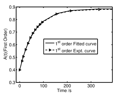
Figure 2: Plot of the experimental and curve with optimized parameters showing the very close fit between the two. The slight difference between the two can probably be attributed to experimental errors.

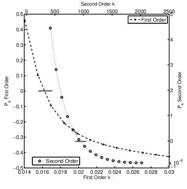
Figure 3: $P_{k}$ functions (9) for reactions (i) and (ii) of order one and two in reaction rate.

5.2 Second order results

To further test our method, we also analyze the second order reaction

$$\mbox{Pu(VI)}+2\mbox{Fe(II)}\,\,\stackrel{{\scriptstyle k_{b}}}{{\longrightarrow}}\,\,\mbox{Pu(IV)}+2\mbox{Fe(III)}$$ (56)

whose rate is given by $\mbox{rate}=k_{0}[\mbox{PuO}^{2+}_{2}][\mbox{Fe}^{2+}]$ where $k_{0}$ is relative to the constancy of other ions in solution such as $\mbox{H}^{+}$. The equations are very different in form to the first-order expressions and serves to confirm the viability of the current method.

For Espenson, the above stoichiometry is kinetically equivalent to the reaction scheme [24, eqn. (2-36)]

$$\mbox{PuO}_{2}^{2+}+\mbox{Fe}^{2+}_{aq}\stackrel{{\scriptstyle k_{b}}}{{\longrightarrow}}\,\mbox{PuO}^{+}_{2}+\mbox{Fe}^{3+}_{aq}.$$

which also follows from the work of Newton et al. [23, eqns. (8,9),p.1429] whose data [23, TABLE II,p.1427] we use and analyze to verify the principles presented here. Espenson had also used the same data as we have to derive the rate constant and other parameters [24, pp.25-26] which is used to check the accuracy of our methodology. The overall absorbance in this case $Y(t)$ is given by [24, eqn(2-35)]

$$Y(t)=\frac{Y_{\infty}+\left\{Y_{0}\left(1-\alpha\right)-Y_{\infty}\right\}\exp(-k\Delta_{0}t)}{1-\alpha\exp(-k\Delta_{0}t)}$$ (57)

where $\alpha=\frac{[\text{A}]_{0}}{[\text{B}]_{0}}$ is the ratio of initial concentrations where $[\text{B}]_{0}>[\text{A}]_{0}$ and $[\text{B}]=[\mbox{Pu(VI)}]$, $[\text{A}]=[\mbox{Fe(II)}]$ and $[\text{B}]_{0}=4.47\times 10^{-5}\text{M}$ and $[\text{A}]_{0}=3.82\times 10^{-5}\text{M}$ . A rearrangement of (57) leads to the equivalent expression [24, eqn(2-34)]

$$\ln\left\{1+\frac{\Delta_{0}\left(Y_{0}-Y_{\infty}\right)}{[\text{A}]_{0}\left(Y_{t}-Y_{\infty}\right)}\right\}=\ln\frac{[\text{B}]_{0}}{[\text{A}]_{0}}+k\Delta_{0}t.$$ (58)

According to Espenson, one cannot use this equivalent form [24, p.25] "because an experimental value of $Y_{\infty}$ was not reported." However, according to Espenson, if $Y_{\infty}$ is determined autonomously, then $k$ the rate constant may be determined. Thus, central to all conventional methods is the autonomous and independent status of both $k$ and $Y_{\infty}$. We overcome this interpretation by defining $Y_{\infty}$ as a function of the total experimental spectrum of $t_{i}$ values and $k$ by inverting (57) to define $Y_{\infty}(k)$ where

$$Y_{\infty}(k)=\frac{1}{N^{\prime}}\sum_{i=1^{\prime}}^{N^{\prime}}\frac{Y_{exp}(t_{i})\left\{\exp(k\Delta_{0}t_{i})-\alpha)\right\}+Y_{0}(\alpha-1)}{(\exp(k\Delta_{0}t_{i})-1)}$$ (59)

where the summation is over all experimental values that does not lead to singularities such as at $t_{i}=0$. In this case, the $\mathbf{P}$ parameter is given by Y${}_{\infty}(k)=P_{1}(k)$, $k_{b}=k$ is the varying $k$ parameter of (4). We likewise define a function $Y_{th}$ of $k$ that is also a function of t, but where the $k$ parameter is interpreted as a "distortion" parameter in the following manner:

$$Y(t,k)_{th}=\frac{Y_{\infty}(k)+\left\{Y_{0}\left(1-\alpha\right)-Y_{\infty}(k)\right\}\exp(-k\Delta_{0}t)}{1-\alpha\exp(-k\Delta_{0}t)}.$$ (60)

In order to extract the parameters $k$ and $Y_{\infty}$ we minimize the square function $Q_{2}(k)$ for this second order rate constant with respect to $k$ given as

$$Q_{2}(k)=\sum_{i=1}^{N}(Y_{exp}(t_{i})-Y_{th}(t_{i},k))^{2}$$ (61)

where the summation is over the experiment $t_{i}$ coordinates. Then the solution to the minimization problem is when the corresponding $P_{k}$ function (9) is zero. The NR method was used to solve $P_{k}=0$ with the error tolerance of $1.0\times 10^{-10}$. With the same notation as in the first order case, the second order results are:
$k_{b}=938.0\pm 18\mbox{(M s)}^{-1}$; $Y_{\infty}=0.0245\pm 0.003$; and $fd=9.606\times 10^{-4}$.

The experimental estimates are [24, p.25]:
$k_{b}=949.0\pm 22\mbox{(M s)}^{-1}$; $Y_{\infty}=0.025\pm 0.003$.

Again the two results are in close agreement. The graph of the experimental curve and the one that derives from our optimization method in given in Fig.(4).

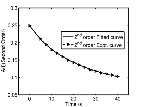
Figure 4: Graph of the experimental and calculated curve based on the current induced parameter-dependent optimization method.

6 Conclusions

The triad of associated implicit function optimization covers both modeling of data and the optimization of arbitrary functions where experimental or theoretical considerations require that a single variable is tagged to a process variable that is iteratively relaxing to equilibrium. Applying method (i)a to chemical kinetics allows for the direct determination of parameters not possible by the standard methodologies used. The results presented here show that for linked variables, it is possible to derive all the parameters associated with a curve by considering only one independent variable which serves as the independent variable for other functions in the optimization process that uses the experimental dataset as function values in the estimation. Apart from possible reduced errors in the computations, it might also be a more accurate way of deriving parameters that are more influenced or conditioned (on physical grounds) by the value of one parameter (such as $k$ here) than others; the current methods that gives equal weight to all the variables might in some cases lead to results that would be considered "unphysical". In complex dynamical systems with multiprocesses, the physical considerations are such that for scientific purposes, it would be advantageous if optimization would be conducted on just one primary coordinate variable, such as in attempting to derive the most general stable conformer in a large molecule, where there are thousands of local minima present if all free coordinate variables are considered [9, Sec.6.7, p.330] . This generalized potential surface might be found suitable for reaction trajectory calculations [9, Ch.4, p.192 on "Features of a landscape"] that require a single path variable, where the general optimized conformer would be relevant to the study of the potential surfaces and force fields present.

7 Acknowledgments

This work was supported by University of Malaya Grant UMRG(RG077/09AFR) and Malaysian Government grant FRGS(FP084/2010A). Cordial discussions concerning real world applications with Gareth Tribello (ASC) is acknowledged. I thank Jorge Kohanoff (ASC) and Christopher Hardacre (Chem. Dept., QUB) for congenial hospitality during this sabbatical.

References

- [1] B.D. Craven. Functions of several variables. Chapman and Hall Ltd, London, 1981.
- [2] J. DePree and C. Swartz. Introduction to Real Analysis. John Wiley & Sons, New York, 1988.
- [3] Tom M. Apostol. Mathematical Analysis. Narosa Publishing House, New Delhi, second edition, 2002.
- [4] W.H. Press, S.A. Teukolsky, W.T. Vetterling, and B.P. Flannery. Numerical Recipes -The Art of Scientific Computing . Cambridge University Press, third edition, 2007.
- [5] J. A. Snyman. Practical Mathematical Optimization: An Introduction to Basic Optimization Theory and Classical and New Gradient-Based Algorithms. Springer Publishing, 2005. ISBN 0-387-24348-8.
- [6] W. C. Davidon. Variable metric method for minimization. SIAM J OPTIMIZ, 1:1–17, 1991.
- [7] C.G. Broyden. The convergence of a class of double-rank minimization algorithms. JIMIA, 6:76–90, 1970.
- [8] A. Banerjee, N. Adams, J. Simons, and J. Shepard. Search for stationary points on surfaces. J. Phys. Chem, 89:52–57, 1985.
- [9] D.A. Wales. Energy Landscapes. Cambridge Molecular Science. Cambridge University Press, Cambridge, England, 2003. Eds:R. Saykally, A. Zewail and D. King.
- [10] S. Kirkpatrick, C. D. Gelatt, and M. P. Vecchi. Optimization by simulated annealing. Science, 220(4598):671–680, 1983.
- [11] D. A. Bates and D. G. Watts. Nonlinear Regression Analysis and its Applications. Wiley Series In Probability And Mathematical Statistics. John Wiley & Sons,Inc., New York, 1988.
- [12] G.H. Golub and V. Pereyra. The differentiation of pseudo-inverses and non-linear least squares problems whose variables separate. J. SIAM, 10:413–432, 1973.
- [13] I. H. M. van Stokkum, D.S. Larsen, and R. van Grondelle. Global and target analysis of time-resolved spectra. BBA, 1657:82–104, 2004. Review.
- [14] P. Shearer and A. C. Gilbert. A generalization of variable elimination for separable inverse problems beyond least squares. INVERSE PROBL, 29:1–27, 2013.
- [15] S. Solar, W. Solar, and N. Getoff. A pulse radiolysis–computer simulation method for resolving of complex kinetics and spectra. Radiat. Phys. Chem., 21(1-2):129–138, 1983.
- [16] A-M Wazwaz. A note on using Adomian decomposition method for solving boundary value problems. Found Phys Lett, 13(5):493–498, 2000.
- [17] J. J. Houser. Estimation of in reaction-rate studies. J. Chem. Educ., 59(9):776–777, 1982.
- [18] P. Moore. Analysis of kinetic data for a first-order reaction with unknown initial and final readings by the method of non-linear least squares . J. Chem. Soc., Faraday Trans. I, 68:1890–1893, 1972.
- [19] W. E. Wentworth. Rigorous least squares adjustment . application to some non-linear equations,I. J. Chem. Educ., 42(2):96–103, 1965.
- [20] W. E. Wentworth. Rigorous least squares adjustment . application to some non-linear equations,II. J. Chem. Educ., 42(3):162–167, 1965.
- [21] C. G. Jesudason. The form of the rate constant for elementary reactions at equilibrium from MD: framework and proposals for thermokinetics. J. Math . Chem, 43:976–1023, 2008.
- [22] Mohammad Niyaz Khan. MICELLAR CATALYSIS, volume 133 of Surfactant Science Series. Taylor & Francis, Boca Raton, 2007. Series Editor Arthur T. Hubbard.
- [23] T. W. Newton and F. B. Baker. The kinetics of the reaction between plutonium(VI) and iron(II). J. Phys. Chem, 67:1425–1432, 1963.
- [24] J. H. Espenson. Chemical Kinetics and Reaction Mechanisms, volume 102(19). McGraw-Hill Book Co., Singapore, second international edition, 1995.