Tearing of Free-Standing Graphene

Abstract

We examine the fracture mechanics of tearing graphene. We present a molecular dynamics simulation of the propagation of cracks in clamped, free-standing graphene as a function of the out-of-plane force. The geometry is motivated by experimental configurations that expose graphene sheets to out-of-plane forces, such as back-gate voltage. We establish the geometry and basic energetics of failure, and obtain approximate analytical expressions for critical crack lengths and forces. We also propose a method to obtain graphene’s toughness. We observe that the cracks’ path and the edge structure produced are dependent on the initial crack length. This work may help avoid the tearing of graphene sheets and aid the production of samples with specific edge structures.

I Introduction

Fracture mechanics provides an ingenious framework by which to assemble experimental information and calculations from continuum elasticity into a theory of material failure. This theory is particularly important for structures that are subject to many design constraints but must be protected against failure at all costs; for example, aircraft Broek (1994).

Graphene is a single layer two-dimensional honeycomb lattice of carbon atoms. It is light, flexible, thermally stable (in a non-oxidizing environment), and has a high electrical conductivity (the Fermi velocity of electrons in graphene is $10^{6}\,\textrm{m/s}$ Gei (2009)). Many experiments have used graphene in the free-standing experimental setup, mostly in an effort to improve electronic properties through absence of a substrate Garcia-Sanchez et al. (2008); Bolotin et al. (2008b, a); Zande et al. (2010); Dorgan et al. (2013)

Graphene is very stiff against in-plane distortions, with a Young modulus on the order of $\approx 1\,\textrm{TPa}$ Lee et al. (2008). Because it is so thin, it is very floppy, and the bending energy is of the order of 1eV Nicklow et al. (1972a). The large value of Young’s modulus gives graphene a very high ideal breaking stress of around 130 GPa, leading to the assertion that it is the strongest material known Lee et al. (2008). This statement is true for defect-free samples. However in practical applications, sample defects are almost inevitable on some scale, and therefore the toughness of graphene is important to determine.

Previous studies of fracture of graphene have employed in-plane geometry Terdalkar et al. (2010); Kim et al. (2011); Lu et al. (2011); Lu and Huang (2010). The energy cracks require to create a new surface in graphene, the fracture toughness, should not be expected to depend upon the precise path by which atoms pull apart around the crack tip, except to the extent that dissipative processes such as generation of phonons is involved Holland and Marder (1999a). Thus in-plane calculations should not be appreciably worse than the out-of-plane calculations we will perform to obtain the fracture toughness of graphene. However, when it comes time to compare with experiment, details of the geometry do matter. Empirical atomic potentials are not necessarily very reliable when it comes to the details of surface energiesHolland and Marder (1999a). Toughness is better obtained from experiment than from theory. To make this determination possible, one needs a geometrical setting where theory and experiment coincide and fracture toughness is the only unknown parameter. Then toughness can be obtained from critical values of force or initial crack length where cracks begin to run.

In some experimental configurations free-standing graphene samples show cracks and holes, and sometimes the samples break Kim et al. (2011); Zande et al. (2010); Ins (2012); Bol (2012); Gol (2012). The back-gate voltage experimental setup is an example. In this case the free-standing graphene sheet is pinned at its edges and suspended between two shelves. The graphene experiences a downward force because the substrate has a voltage different from the graphene itself. We perform molecular dynamics simulations in this geometry, employing nanometer scale samples. From these simulations, we deduce the basic geometry of the failure process. With the understanding of the geometry in hand, we develop analytical approximations that can be employed on samples of any size where failure occurs in the same mode. We verify that our simulations are in satisfactory accord with these approximations.

The structure of this article is as follows: In Section II we describe our simulations and point out the essential way that sheets deform in the presence of uniform downward forcing to drive crack motion. In Section III we develop analytical expressions to correspond to this geometry. In Section IV we compare our analytical expressions with our simulations and the available experimental evidence to estimate fracture toughness of graphene. Section V contains final discussion and conclusions.

II Numerical study

Here we present a numerical study of the propagation of cracks in clamped, free-standing graphene as a function of the out-of-plane force. We use the MEAM semi-empirical potential Baskes (1992), shown to reproduce well the properties of graphene Thompson-Flagg et al. (2009); Lee and Lee (2005) and to support crack propagation Holland and Marder (1999b). The energy minimization is done through damped molecular dynamics. To better model experimental conditions, all the simulations in this work are of finite-sized graphene sheets, and no periodic boundary conditions are used. The simulations were done at zero temperature so as to focus on fracture mechanics. We saw no indication during the investigation of phenomena such as lattice trapping where thermal fluctuations would have been important to overcome energy barriers.

Cracks on graphene sheets have been observed to come in multiple sizes and shapes Zande et al. (2010). Most experiments focus on electronic properties, and do not look at initial cracks on the samples. Consequently, the shapes of the cracks are in general unknown. We consider two possible initial conditions: a crack in the middle of the sheet and a crack at the very edge of the sheet. The first because it is a symmetrical problem and the second because defects can occur where the graphene sheet meets the support that suspends it.

We start with a flat graphene sheet, where the position of the atom $i$ is represented by $(x_{0}^{i},y_{0}^{i},z_{0}^{i})$. We consider a straight crack that runs parallel to the x-axis and has a length of $x_{cut}$. To provide a seed configuration we keep the $x$ and $y$ position of the atom and change $z$ by

$$z^{i}=z^{i}_{0}-P_{A}\left(1-\exp{(P_{B}\cdot y_{0}^{i})}\right)\cdot\left(1-\exp{(P_{B}(-x_{0}^{i}+x_{cut}))}\right)$$ (1)

The parameters $P_{A}$ and $P_{B}$ determine the initial curvature of the sheet. As an example of an initial condition, Fig. 1a shows a crack of $l\approx$ 10Å at the edge of a suspended graphene sheet. The clamped edges are not allowed to move and where chosen to have a width of $\approx$ 5Å.

During the initial molecular dynamics time steps the sample relaxes, as shown in Fig.1b. Given sufficient time in the absent of external forces, the crack would zip back up and the sample would heal. This does not happen because we apply a downward force to every atom in the sheet. For samples where sufficient force is applied, the crack starts running, as seen in Fig. 1c. Short movies of crack propagation are available at Moura and Marder .

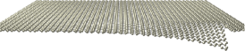
(a) initial crack of $l\approx$ 10Å

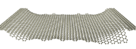
(b) sheet wrinkles and bends

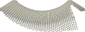
(c) crack propagates

Figure 1: Constant downward force is applied on a 100Å by 100Å clamped, free-standing graphene sheet with an initial crack of $l\approx$ 10Å. Notice that the sheet wrinkles and bends before the crack runs.

We do not know what creates cracks in graphene sheets in actual experiments. They result from impurities, defects, or details of sample preparation. We emphasize that in the theory of fracture mechanics, crack propagation is independent of the mechanism that initially creates the crack.

We encountered some difficulties in determining the period of time that it takes for a crack to begin to run. The simulations show that first the sheet ripples and bends, and then the crack runs. In terms of energy, what we see is an initial large drop in potential and kinetic energy, Fig. 2. Then the sheet reaches an almost-stable state, where the energy almost plateaus, decreasing very slowly. Finally, when the crack runs, another drop in potential energy occurs together with a fast increase in kinetic energy. If the force applied is not strong enough for the crack to run, the sheet stays in the bent state forever. Numerically we have to set an acceptable period of time to be considered “forever”. We observe that longer initial crack lengths lead to longer periods of time spent in the almost-stable state. After studying many simulations we decided that 600,000 time steps $=1.5\times 10^{-10}$ s is, in most cases, an acceptable period of time to study the crack propagation (or lack of it).

Figure 2: Potential energy vs time for an initial edge crack of $l\approx$ 35Å. The first large drop in potential energy happens while the sheet ripples and bends. Then potential energy slowly decreases as the ripples disappear and the sheet reaches its fully bent state. Another fast drop in potential energy occurs when the crack starts running.

The numerical simulations show the basic geometry of the failure process. In both cases, cracks at the edge and in the middle of the sheet, we observe that the sheet folds in a crease (on both sides of the crack) before the crack runs, Fig. 3. In the next section we use this geometry to obtain approximate analytical expressions for critical crack lengths and forces.

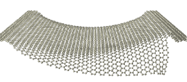
(a) initial edge crack of $l\approx$ 20Å

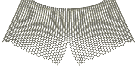
(b) initial middle crack of $l\approx$ 25Å

Figure 3: Clamped, free-standing graphene sheets with an initial crack (at the edge and in the middle) under a downward constant force. In both cases the sheet exhibits a crease before the crack runs. The crease goes from the crack tip essentially all the way to the fixed end.

III Analytical approach to tearing a two dimensional sheet

The system of interest is a two dimensional sheet, such as graphene, with an initial crack of length $l$. The sheet is suspended and exposed to a uniform downward force $f$. The problem is to describe the propagation of a crack in such sheet and the minimum force required for the crack to run.

Here we follow a procedure similar to the one developed by Marder Marder (2004) for the propagation of a crack in a 3D strip, making the appropriate changes for our two dimensional problem.

Consider a system with an initial crack of length $l$ and total energy $U_{tot}(l)$, Fig. 4. The crack can run a length $dl$ if doing so reduces the total energy of the system; that is:

$$U_{tot}(l)>U_{tot}(l+dl)$$ (2)

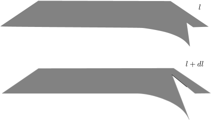
Figure 4: Top image: Clamped, free-standing two dimensional sheet with an initial crack of length $l$ at the right hand side. The sheet is clamped at the left and right edges. Bottom image: Because of an external downward force the crack runs, a length $dl$, and the sheet bends diagonally.

The total energy of the system can be written as the energy contained within the crack tip region plus the energy outside of it, $U_{out}$. The energy to move the crack tip (region) is proportional to the energy of the new surface opened up by the crack. Therefore the total energy of a 2D sheet, such as graphene, with a crack of length $l$ is given by:

$$U_{tot}(l)=\Gamma l+U_{out}(l)$$ (3)

where $\Gamma$ is the fracture toughness. The fracture toughness is material-dependent, and it can be measured experimentally (and obtained numerically).

From Eqs. (2) and (3) we get Griffith’s criterion for a crack to propagate in a 2D sheet:

$$\frac{dU_{out}}{dl}+\Gamma<0.$$ (4)

This should be understood as a necessary but not sufficient condition for crack motion. Atomic systems can exhibit lattice trapping, where cracks become stuck between atoms and do not propagate even though there is enough energy available to allow it Hsieh and Thomson (1973). This phenomenon leads to hysteresis depending upon whether the driving force for crack motion is increasing or decreasing. As we ramped external forces both up and down and saw cracks run forward or heal backward at very nearly the same force, provided we waited long enough, we do not think lattice trapping is very important in this case. We analyze the fracture mechanics of the two geometries under consideration: a crack at the very edge of the sheet and a crack in the middle of the sheet.

III.1 Analytical study of a sheet with an edge crack

For an initial crack at the edge of the sheet the downward force will tear the sheet at the edge making it bend diagonally, as seen on Fig. 4. The energy outside the crack tip, $U_{out}$, is then equivalent to the energy required to bend a 2D sheet.

First, we consider the energy needed to bend a strip (Fig. 5). Then we extend the result to the 2D case of a bending sheet.

Figure 5: One dimensional strip of length $L$, fixed at one end, and bending due to an external downward force.

III.1.1 Energy for a bending strip

The energy of a 1D strip of length $L$ under a downward force $f$ is given by:

$$U^{1D}=\int_{0}^{L}ds\left[\frac{k_{l}}{2}\left(\frac{d\theta}{ds}\right)^{2}+f_{l}\cdot y(s)\right]$$ (5)

where $k_{l}$ is the bending modulus (times length). The $\theta$ term refers to the bending energy and the $f_{l}$ term refers to energy due to the external downward force (per length) applied to the strip. From Fig. 5 we observe that:

$$y(s)=\int\sin(\theta)ds$$ (6)

Therefore:

$$U^{1D}=\int_{0}^{L}ds\left[\frac{k_{l}}{2}\left(\frac{d\theta}{ds}\right)^{2}+f_{l}\int_{0}^{s}\sin(\theta(s^{\prime}))ds^{\prime}\right]$$ (7)

To obtain the energy outside the crack tip in terms of the minimum force required for the crack to run we need to minimize Eq. (7), which results in (see Appendix A for details):

$$U^{1D}=2\left(2-\sqrt{2}\right)\sqrt{f_{l}k_{l}L}-\frac{1}{2}f_{l}L^{2}$$ (8)

The first term refers to the folding of the strip and the second term to the potential energy. We note that the folding energy depends, somewhat surprisingly, on the total length $L$ of the strip. This happens because as the strip length increases so does the force on it, and the crease bends at a tighter and tighter angle.

III.1.2 Energy for a bending sheet

Now we obtain approximate expressions for a sheet folding from the crack tip all the way to the fixed end, forming a crease as seen in Fig. 6. We consider the bending energy for a right triangle, with one side of length $l$, the crack length, and another side of length $m$, the horizontal width of the crease.

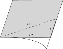
Figure 6: Suspended sheet with an initial crack of length $l$. The triangle formed by the crease is the part of the sheet that is initially free to bend, as it is not attached to the support.

Figure 7: Relabeling Fig.6: right triangle formed by the crease, $n=n_{1}+n_{2}$, the crack length, $l$, and the horizontal width of the crease, $m$. Note that the horizontal width of the crease, $m$, is essentially the width of the sheet.

In the previous section we obtained the energy of a bending strip under a downward force. We can now integrate that result over the right triangle to obtain the bending energy of a triangle. We break the triangle into two parts (Fig. 7) and obtain:

$$U^{2D}=U_{1}+U_{2}$$ (9)

where:

$$U_{1}=\int_{0}^{n_{1}}dr_{1}\int_{0}^{L(r_{1})}ds\left[\frac{k}{2}\left(\frac{d\theta}{ds}\right)^{2}+f_{a}\int_{0}^{s}\sin(\theta(s^{\prime}))ds^{\prime}\right]$$ (10)

and

$$U_{2}=\int_{0}^{n_{2}}dr_{2}\int_{0}^{L(r_{2})}ds\left[\frac{k}{2}\left(\frac{d\theta}{ds}\right)^{2}+f_{a}\int_{0}^{s}\sin(\theta(s^{\prime}))ds^{\prime}\right].$$ (11)

Here $f_{a}$ is the downward force per area and $k$ is the bending modulus (units of energy).

Notice that, in the two-dimensional case, the total bending length, $L(r)$, varies throughout the triangle, and is written as $L(r_{1})=({h}/{n_{1}})r_{1}$ for the first triangle, and $L(r_{2})=({h}/{n_{2}})r_{2}$ for the second triangle. The height of the triangle is given by $h={m\cdot l}/{\sqrt{m^{2}+l^{2}}}$ and the hypotenuse by $n=n_{1}+n_{2}=\sqrt{m^{2}+l^{2}}$ (see Fig. 7).

The first integral is the same as the one we solved for the 1D case of the bending strip. Therefore, in the case of $U_{1}$ for example:

$$U_{1}=\int_{0}^{n_{1}}dr_{1}\left[2\left(2-\sqrt{2}\right)\sqrt{kf_{a}L(r_{1})}-\frac{1}{2}f_{a}L^{2}(r_{1})\right]$$ (12)

Substituting $L(r_{1})=hr_{1}/n_{1}$ and solving the integral in $r_{1}$ we obtain:

$$U_{1}=n_{1}\left[\frac{4}{3}\left(2-\sqrt{2}\right)\sqrt{kf_{a}h}-\frac{1}{6}f_{a}h^{2}\right]$$ (13)

As $U_{2}$ is analogous to $U_{1}$, Eq. (9) results in:

$$U^{2D}=U_{1}+U_{2}=(n_{1}+n_{2})\left[\frac{4}{3}\left(2-\sqrt{2}\right)\sqrt{kf_{a}h}-\frac{1}{6}f_{a}h^{2}\right]$$ (14)

Substituting $n=n_{1}+n_{2}=\sqrt{m^{2}+l^{2}}$ and $h=\frac{ml}{\sqrt{m^{2}+l^{2}}}$, we obtain that the energy required to bend a right triangle is given by:

$$U^{2D}=C\sqrt{kf_{a}nml}-\frac{1}{6}f_{a}\frac{m^{2}l^{2}}{n}$$ (15)

where $C=\frac{4}{3}\left(2-\sqrt{2}\right)$, $f_{a}$ is the downward force per area, $k$ is the bending modulus, $m$ is the horizontal width of the crease, $l$ is the crack length, and $n=\sqrt{m^{2}+l^{2}}$. Note that, the first term refers to the folding of the sheet and the second term to the potential energy.

III.2 Griffith Point

In the beginning of Sec. III we presented Griffith’s criterion for a crack to propagate on a 2D sheet:

$$\frac{dU_{out}}{dl}+\Gamma=0$$

Substituting the energy outside the crack tip, $U_{out}$, for the energy to bend a triangle $U^{2D}$, Eq. (15), and solving for the minimum force (per area) for the crack to run, we obtain our final expression for an edge crack:

$$f_{a}^{edge}=\frac{3(l^{2}+m^{2})^{3/2}}{2l^{3}m^{3}(l^{2}+2m^{2})^{2}}\Big{[}3C^{2}k(2l^{2}+m^{2})^{2}+4\Gamma l^{2}m(l^{2}+2m^{2})$$

$$+C(2l^{2}+m^{2})\sqrt{3k(3C^{2}k(2l^{2}+m^{2})^{2}+8\Gamma l^{2}m(l^{2}+2m^{2}))}\Big{]}$$ (16)

where $k$ is the bending modulus Nicklow et al. (1972b); Khare et al. (2007); Thompson-Flagg et al. (2009); Fasolino et al. (2007), $\Gamma$ is the fracture toughness, $C=\frac{4}{3}\left(2-\sqrt{2}\right)$, $l$ is the crack length, and $m$ is the horizontal width of the crease. See Fig. 6. Note that the horizontal width of the crease, $m$, is essentially the width of the sheet.

For a crack in the middle of the sheet, as there are two folds, the total energy outside the crack tip is:

$$U_{out}=2\cdot U^{2D}$$ (17)

Hence our final expression for a crack in the middle of the sheet is:

$$f_{a}^{middle}=\frac{3(l^{2}+\tilde{m}^{2})^{3/2}}{2l^{3}\tilde{m}^{3}(l^{2}+2\tilde{m}^{2})^{2}}\Big{[}3C^{2}k(2l^{2}+\tilde{m}^{2})^{2}+2\Gamma l^{2}\tilde{m}(l^{2}+2\tilde{m}^{2})$$

$$+C(2l^{2}+\tilde{m}^{2})\sqrt{3k(3C^{2}k(2l^{2}+\tilde{m}^{2})^{2}+4\Gamma l^{2}\tilde{m}(l^{2}+2\tilde{m}^{2}))}\Big{]}$$ (18)

where $\tilde{m}$ is essentially half the width of the sheet for a sheet with crack in the middle.

For initial cracks that are much smaller than the width of the sheet ($l<<m$) we find:

$$f_{a}^{edge_{l<<m}}=3\frac{\Gamma}{ml}+\frac{3C}{8l^{3}}\left[3Ck+\sqrt{3k\left(3C^{2}k+16\Gamma\frac{l^{2}}{m}\right)}\right]$$ (19)

and:

$$f_{a}^{middle_{l<<\tilde{m}}}=\frac{3}{2}\frac{\Gamma}{\tilde{m}l}+\frac{3C}{8l^{3}}\left[3Ck+\sqrt{3k\left(3C^{2}k+8\Gamma\frac{l^{2}}{\tilde{m}}\right)}\right]$$ (20)

It is intuitive that the force required for a crack to run will depend on the initial crack length. For sheets of paper, for example, it is easier to tear a sheet with a long crack, than to tear one with a short crack. Note that the expressions for the minimum force required for a crack to run, Eq. (16) and (18), depend not only on the crack length, $l$, but also on the width of the sheet, $m$, (or the half-width, $\tilde{m}$). Fig. 8 shows two graphs of force versus initial crack length for a sheet with a crack in the middle. The half width of the sheet, $\tilde{m}$, in Fig. 8b is 10 times larger than the one in Fig. 8a. Notice that longer initial crack lengths lead to lower minimum forces. Also, wider sheets lead to lower minimum forces. As a result, the minimum force approaches zero with increasing initial crack length and width of the sheets.

(a) $\tilde{m}=50\times 10^{-10}$meters

(b) $\tilde{m}=500\times 10^{-10}$meters

Figure 8: Plot of force (in Newtons per atom) versus initial crack length (in meters), Eq. (18). The half width of the sheet, $\tilde{m}$, in Fig. 8b is 10 times larger than the one in Fig. 8a. Note how the minimum force decreases with increasing initial crack length and width of the sheets.

IV Comparison between numerical and analytical results

To compare the numerical results with the analytical expression, Eqs. (16,18), we need the values of the bending modulus $k$ and the fracture toughness $\Gamma$ for graphene.

The experimental value of the bending modulus of graphene is $k_{exp}=1.2\textrm{eV}$ Nicklow et al. (1972b). In previous numerical work on ripples in graphene we found $k=1.77$eV Thompson-Flagg et al. (2009). Another numerical study, by Fasolino et al. Fasolino et al. (2007), obtained $k=1.1$eV.

We have not been able to find an experimental measurement of graphene’s fracture toughness in the literature. From our simulations we obtained:

$$\Gamma_{numerical}\approx 3.82\times 10^{-9}\textrm{J/m}$$ (21)

For the full numerical calculation of graphene’s fracture toughness see Appendix B.

The uniform downward force is applied to every atom on the sheet, therefore numerically we use force per atom $f_{atom}$, and not force per area $f_{a}$, as in the analytical calculations. The relationship between force per atom and force per area is:

$$f_{atom}=\frac{f_{a}}{\eta}=\frac{f_{a}}{38.17\times 10^{18}\textrm{m}^{-2}}$$ (22)

where $\eta=38.17\times 10^{18}\textrm{m}^{-2}$ is the number of atoms per area in graphene.

IV.1 Numerical study of a sheet with a crack in the middle

A graph of force per atom versus initial crack length for a crack in the middle of the sheet is shown in Fig. 9 The line is the theoretical expression, Eq. (18), and the dots are the numerical results. The horizontal error bars are estimated uncertainties of the initial crack length due to the fact that the crack tip is not perfectly well defined. The vertical error bars reflect the precision of our numerical simulations.

Fig. 9 shows good agreement between the theory and the simulations, except for some of the longer cracks in systems of overall size 100Å by 100Å. Discrepancies between theory and numerics should be expected as crack lengths approach system dimensions. To verify that system size effects were responsible we simulated the same initial crack lengths in a sheet of 200Å by 100Å; that is, we kept the same width, $m$, and changed only the sheet’s length, a parameter that does not appear in the theory. The results are shown in Figs. 9 and 10. The line is the theoretical expression, Eq. (18), the dots are the numerical results for a sheet of 100Å by 100Å, and the open circle are the numerical results for a sheet of 200Å by 100Å. Notice that for short initial cracks both results fall exactly on top of each other. For longer initial cracks the force plateaus for the 200Å by 100Å sheet, as in the theory, while for the 100Å by 100Å sheet the force decreases due to edge effects.

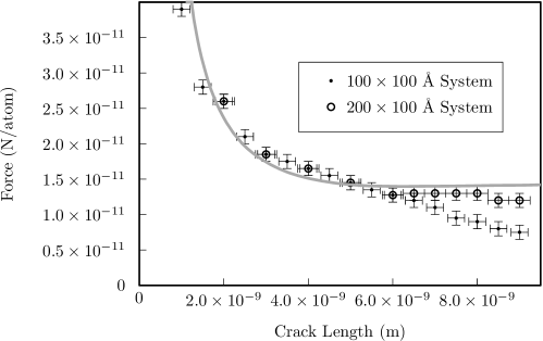
Figure 9: Graph of force (in Newtons per atom) vs initial crack length (in meters) for a crack in the middle of the sheet. The line is the theoretical expression, Eq. (18), the dots are the numerical results for a sheet of 100Å by 100Å, and the open circles are the numerical results for a sheet of 200Å by 100Å.

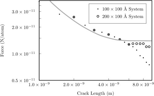
Figure 10: Log-log graph of force (in Newtons per atom) vs initial crack length (in meters) for a wide-open middle crack. The line is the theoretical expression, Eq. (18), the dots are the numerical results for a sheet of 100Å by 100Å, and the open circles are the numerical results for a sheet of 200Å by 100Å.

Another issue is that it is hard to produce short initial cracks in the middle of the sheet. They close easily and the uncertainty of the crack tip plays an important role. Therefore, the uncertainties for the first two points on the graphs (initial cracks of 10Å and 15Å) perhaps should be higher than the values presented on Fig. 9

IV.2 Numerical study of sheet with an edge crack

Cracks at the edge of the sheet present some interesting characteristics, not seen in cracks in the middle of the sheet. The simulations show that, depending on the initial condition, a crack will not run straight through the sheet, as initially expected (see Fig. 11 and Fig. 12). Short initial cracks run straight, while longer cracks do not.

Another interesting result is that, depending on the initial crack length and orientation (zigzag or armchair), the propagation pattern will be different (see Fig. 11 and Fig. 12). Similar dynamics have been seen in simulations of tearing graphene nanoribbons Kawai et al. (2009).

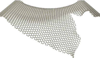
Figure 11: Non-straight crack propagation in a 100Å by 100Å graphene sheet with an initial crack of $l\approx$ 25Å. Note that the initial zigzag crack propagates as armchair.

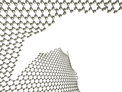
Figure 12: Non-straight crack propagation in a 100Å by 100Å graphene sheet with an initial crack of $l\approx$ 30Å. Note that the initial zigzag crack propagates along the ’armchair’ direction and then turns along the ’zigzag’ direction.

Fig. 13 shows a log-log graph of force per atom versus initial crack length. The dotted line is the theoretical expression, Eq. (16), and the disks are the numerical results. Theory and numerical results do not agree very well.

Looking at the simulations of sheets with an initial edge crack we notice that the crease seems to end before the fixed end: see Fig. 14. This means that the value for $m$ should be smaller than the width of the sheet (minus the width of both fixed ends). The best fit for the theoretical expression Eq. (16) with the numerical results, assuming $m$ to be a fitting parameter, is shown as the solid line in Fig. 13. The width of the sheet minus the clamped region is $\approx$ 90Å and the best fit value for $m$ is 64Å. It was difficult to determine the crease length from the simulations, so we treated it as a fitting parameter, obtaining very reasonable results.

Figure 13: Log-log graph of force vs initial crack length for an edge crack. The dotted line shows Eq. (16), taking $m$ to be the width of the sheet minus the clamped region; the solid line is the best fit for theoretical expression, Eq. (16), assuming $m$ to be a fitting parameter and the disks are numerical results. The width of the sheet minus the clamped region is 90Å and the best fit value for $m$ is 64Å.

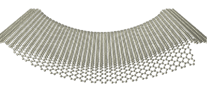
(a) initial edge crack of $l\approx$ 10Å

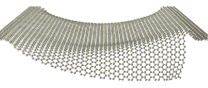
(b) initial edge crack of $l\approx$ 25Å

Figure 14: Clamped, free-standing graphene sheets with an initial edge crack under a downward constant force. The sheets exhibits a crease before the crack runs. The crease starts at the crack tip and ends before the fixed end.

V Conclusion

We presented a numerical and an analytical study of the propagation of cracks in clamped, free-standing graphene as a function of the out-of-plane force. The geometry is motivated by experimental configurations that expose graphene sheets to out-of-plane forces, such as the back-gate voltage. We studied two different initial conditions: a crack at the edge of the sheet and a crack in the middle of it.

We obtained approximate analytical expressions for the minimum force required for a crack to run. These expressions depend on the initial crack length, as expected, but also on the width of the graphene sample. The minimum force decreases with increasing initial crack length and increasing width of the sheets.

The numerical fracture forces show good agreement with the analytical fracture forces for cracks in the middle of the sheet. For cracks at the edge the numerical results and the theory do not agree as well, unless we consider crease configurations that do not reach all the way to the edge of the sample. The simulations show that depending on the initial condition a crack will not run straight through the sheet, as initially expected. Initial cracks in the middle of the sheet always run straight, while initial cracks at the edge do not.

Depending on the initial crack orientation (zigzag or armchair), the propagation pattern will be different. Similar dynamics have been seen in simulations of tearing graphene nanoribbons Kawai et al. (2009) and in experiments, see Fig. 15. The edge orientation of a graphene sheet determines its electronic properties, therefore it will be most useful to be able to predict the edge orientation of produced samples.

Another interesting numerical result is that the sheet folds in a crease before the crack runs, both for sheets with a crack in the middle (on both sides of the crack) and at the edge, Fig. 3. In experiments, folds, scrolls, and creases are commonly observed in free-standing graphene samples, see Fig. 16.

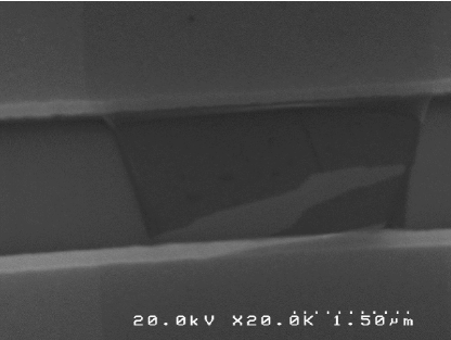
Figure 15: Top view: SEM image of free-standing CVD graphene. Note the crack runs from the edge to the middle of the sheet, making sharp turns, similar to our simulations. Image courtesy of the Bolotin Research Group.

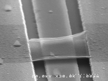
Figure 16: SEM image of free-standing CVD graphene. Note the crack at the left edge and the crease that runs all the way to the right edge, similar to what we observe in our simulations. Image courtesy of the Bolotin Research Group.

It has been difficult to gather experimental data on this problem, because the fracture of free-standing graphene sheets is in general an undesirable occurrence. Therefore most experiments do not report or take measurements of such events. Preliminary results Bol (2012) show that, for initial crack lengths of about 10% of the graphene sample’s length, our expression for the minimum force required for a crack to run, Eq. (16) and (18), results in forces comparable to the forces a free-standing graphene is subjected to in a back-gate voltage experiment.

In particular, for samples of roughly 2$\mu$m by $2\mu$m, fracture was sometimes observed with back-gate voltages of 2-3 V with the sample at a height of 150 nm above the substrate. We estimate an electric field of $20\times 10^{6}$ V/m, leading to a force per atom of $10^{-16}N$/atom. According to our calculations, this force is too small to cause fracture for seed cracks of reasonable length. For this value of the force per atom, we would need a seed crack of length $1.5\mu$m. Alternatively, for seed cracks of length $0.2\mu$m, we would not expect fracture until the force reached $8\times 10^{-16}N$/atom. While this discrepancy is admittedly large, we note that we are working without an experimental value for fracture toughness, and that classical potentials can easily lead to inaccurate values for this quantity.

The analytical expressions for the the minimum force required to tear a two dimensional sheet, such as graphene, in terms of the initial crack length, offer insight into the tearing of graphene, and suggest the order of magnitude for the forces to be used or avoided in experiments. Also, experiments can obtain the value for the tearing fracture toughness of graphene (a quantity we have not been able to find in the literature) by combining our theory with measurements of initial crack length and applied force.

Appendix A Energy for bending a 1D strip

The energy of a 1D strip of length $L$ under a downward force $f_{l}$ is given by (Eqs. (5) and (6)):

$$U^{1D}=\int_{0}^{L}ds\left[\frac{k_{l}}{2}\left(\frac{d\theta}{ds}\right)^{2}+f_{l}\int_{0}^{s}\sin(\theta(s^{\prime}))ds^{\prime}\right]$$ (23)

Note that $s^{\prime}$ is just a variable (not a derivative of $s$).

We need to minimize Eq. (7) to obtain the energy outside the crack tip in terms of the minimum force required for the crack to run. To find the minimum (or the maximum) of $U^{1D}$ we take the functional derivative and make it equal to zero:

$$\lim_{\epsilon->0}\frac{U^{1D}(\theta+\epsilon\phi)-U^{1D}(\theta)}{\epsilon}=0$$ (24)

This results in:

$$\lim_{\epsilon->0}\frac{1}{\epsilon}\int_{0}^{L}ds\left\{\frac{k_{l}}{2}\left[2\epsilon\frac{d\phi}{ds}\frac{d\theta}{ds}+\epsilon^{2}\left(\frac{d\phi}{ds}\right)^{2}\right]+f_{l}\int_{0}^{s}\left[\sin(\theta(s^{\prime})+\epsilon\phi(s^{\prime}))-\sin(\theta(s^{\prime}))\right]ds^{\prime}\right\}=0$$ (25)

Expanding the sine function in a Taylor series we obtain:

$$\lim_{\epsilon->0}\frac{1}{\epsilon}\int_{0}^{L}ds\left\{\frac{k_{l}}{2}\left[2\epsilon\frac{d\phi}{ds}\frac{d\theta}{ds}+\epsilon^{2}\left(\frac{d\phi}{ds}\right)^{2}\right]+f_{l}\int_{0}^{s}\left[\epsilon\phi(s^{\prime})\cos(\theta(s^{\prime}))+O(\epsilon^{2})\right]ds^{\prime}\right\}=0$$ (26)

Dividing by $\epsilon$ and taking the limit as it goes to zero:

$$\int_{0}^{L}ds\left\{\frac{k_{l}}{2}2\frac{d\phi}{ds}\frac{d\theta}{ds}+f_{l}\int_{0}^{s}\phi(s^{\prime})\cos(\theta(s^{\prime}))ds^{\prime}\right\}=0$$ (27)

Using integration by parts on the first term and the fact that $\phi$ vanishes at 0 and L:

$$\int_{0}^{L}ds\left\{-k_{l}\phi\frac{d^{2}\theta}{ds^{2}}+f_{l}\int_{0}^{s}\phi(s^{\prime})\cos(\theta(s^{\prime}))ds^{\prime}\right\}=0$$ (28)

The result should be independent of the test function $\phi$. Here we choose $\phi=\delta(s-s^{\prime\prime})$:

$$\int_{0}^{L}ds\left\{-k_{l}\delta(s-s^{\prime\prime})\frac{d^{2}\theta}{ds^{2}}+f_{l}\int_{0}^{s}\delta(s^{\prime}-s^{\prime\prime})\cos(\theta(s^{\prime}))ds^{\prime}\right\}=0$$ (29)

After some algebra we obtain:

$$-k_{l}\frac{d^{2}\theta(s^{\prime\prime})}{ds^{\prime\prime 2}}+f_{l}\cos(\theta(s^{\prime\prime}))(L-s^{\prime\prime})=0$$ (30)

Note that $s^{\prime\prime}$ is just a variable (not the second derivative of $s$). At this point an appropriate approximation needs to be considered in order to solve this equation analytically.

A.0.1 One-dimensional crease energy

Here we consider the limit $L\rightarrow\infty$, since by the time $s^{\prime\prime}$ is comparable to $L$, $\theta=-\pi/2$. Eq. (30) then simplifies to:

$$-k_{l}\frac{d^{2}\theta(s^{\prime\prime})}{ds^{\prime\prime 2}}+f_{l}\cos(\theta(s^{\prime\prime}))L=0$$ (31)

After some manipulation we obtain:

$$\frac{d\theta(s^{\prime\prime})}{ds^{\prime\prime}}=\sqrt{2\frac{f_{l}L}{k_{l}}\sin(\theta(s^{\prime\prime}))-C_{1}}$$ (32)

where $C_{1}$ is a constant, and it can be determined from the following conditions:

$$\frac{d\theta}{ds^{\prime\prime}}(L)=0$$

$$s^{\prime\prime}\rightarrow L,\theta\rightarrow-\frac{\pi}{2}$$

The result is:

$$C_{1}=2\frac{f_{l}L}{k_{l}}\sin(\theta(L))=2\frac{f_{l}L}{k_{l}}\sin\left(-\frac{\pi}{2}\right)=-2\frac{f_{l}L}{k_{l}}$$ (33)

Inserting into Eq. (32) one obtains

$$\frac{d\theta(s^{\prime\prime})}{ds^{\prime\prime}}=\sqrt{2\frac{f_{l}L}{k_{l}}\left[\sin(\theta(s^{\prime\prime}))+1\right]}.$$ (34)

Substituting

$$\theta(s^{\prime\prime})=\frac{\pi}{2}-\Phi(s^{\prime\prime})$$ (35)

and using trigonometric identities, we obtain:

$$\frac{d\Phi(s^{\prime\prime})}{ds^{\prime\prime}}=-2\sqrt{\frac{f_{l}L}{k_{l}}}\cos(\Phi(s^{\prime\prime})/2)$$ (36)

After some manipulation we have

$$\Phi(s^{\prime\prime})=2\arccos\left(\operatorname{sech}\left(\sqrt{\frac{f_{l}L}{k_{l}}}s^{\prime\prime}-C_{2}\right)\right)$$ (37)

where $C_{2}$ is a constant to be determined.

Using Eq. (35) we can go back to $\theta$:

$$\theta(s^{\prime\prime})=\frac{\pi}{2}-2\arccos\left(\operatorname{sech}\left(\sqrt{\frac{f_{l}L}{k_{l}}}s^{\prime\prime}-C_{2}\right)\right)$$ (38)

Applying the condition that $\theta(0)=0$, we obtain the expression for the bending function of a 1D strip

$$\theta(s^{\prime\prime})=\frac{\pi}{2}-2\arccos\left(\operatorname{sech}\left(\sqrt{\frac{f_{l}L}{k_{l}}}s^{\prime\prime}+\operatorname{arccosh}\left(\sqrt{2}\right)\right)\right).$$ (39)

Now that we have $\theta$ we insert it back in the expression for the energy of a 1D strip, Eq. (23), and find

$$\ U^{1D}=-2\sqrt{2}\sqrt{f_{l}k_{l}L}$$

$$+\frac{2k_{l}}{L}\ln\left[\cosh\left(\sqrt{\frac{f_{l}L^{3}}{k_{l}}}\right)+\frac{1}{\sqrt{2}}\sinh\left(\sqrt{\frac{f_{l}L^{3}}{k_{l}}}\right)\right]$$

$$+2\sqrt{f_{l}k_{l}L}\tanh\left(\sqrt{\frac{f_{l}L^{3}}{k_{l}}}+\operatorname{arccosh}\left(\sqrt{2}\right)\right)-\frac{1}{2}f_{l}L^{2}.$$ (40)

Looking at the asymptotic behavior for large $L$

$$U^{1D}=2\left(2-\sqrt{2}\right)\sqrt{f_{l}k_{l}L}-\frac{1}{2}f_{l}L^{2}$$ (41)

we finally arrive to the result presented in Eq. (8).

Appendix B Numerical calculation of graphene’s fracture toughness $\Gamma$

The growth of a crack requires the creation of two new surfaces and hence an increase in the fracture toughness (i.e. surface energy). As graphene is a two-dimensional sheet the new surfaces are actually edges and the fracture toughness is given by energy per length, and not the usual energy per area.

Numerically we can find the energy to create a new surface by simply separating the sheet from its fixed edges. This energy only depends on the interaction between atoms, obtained from the MEAM potential. Therefore here we do not apply a downward force, we do not have initial cracks, and no molecular dynamics is done. We start by fixing two sides of a graphene sheet. Then we move the rest of the sheet downward. Every time step the atoms are moved down by the same distance. The sheet moves farther and farther away from its fixed ends until finally the new surfaces are created, Fig. 17. The fracture toughness $\Gamma$ is then given by the change in energy divided by the length of the two edges created:

$$\Gamma_{numerical}=\frac{(E_{final}-E_{initial})}{\textrm{2 $\times$ edge length}}\approx 3.82\times 10^{-9}\textrm{J/m}.$$ (42)

This calculation does not substitute an experimental measurement of the fracture toughness. It is fundamental to the theory of fracture that the fracture toughness be measured experimentally. We have not been able to find experimental values for this quantity in the literature.

Figure 17: Graph of energy per length (in Joules per meter) vs downward distance (in meters).

References

- Broek (1994) D. Broek, The Practical Use of Fracture Mechanics (Kluwer Academic Press, Dordrecht, 1994), 3rd ed.
- Gei (2009) (2009), private communication with Andre Geim.
- Bolotin et al. (2008a) K. I. Bolotin, K. J. Sikes, J. Hone, H. L. Stormer, and P. Kim, Physical Review Letters 101, 096802 (2008a), URL http://link.aps.org/doi/10.1103/PhysRevLett.101.096802.
- Bolotin et al. (2008b) K. Bolotin, K. Sikes, Z. Jiang, M. Klima, G. Fudenberg, J. Hone, P. Kim, and H. Stormer, Solid State Communications 146, 351 (2008b), ISSN 0038-1098, URL http://www.sciencedirect.com/science/article/pii/S00381098080%01178.
- Garcia-Sanchez et al. (2008) D. Garcia-Sanchez, A. M. van der Zande, A. S. Paulo, B. Lassagne, P. L. McEuen, and A. Bachtold, Nano Lett. 8, 1399 (2008), ISSN 1530-6984, URL http://dx.doi.org/10.1021/nl080201h.
- Zande et al. (2010) A. M. v. d. Zande, R. A. Barton, J. S. Alden, C. S. Ruiz-Vargas, W. S. Whitney, P. H. Q. Pham, J. Park, J. M. Parpia, H. G. Craighead, and P. L. McEuen, Nano Letters 10, 4869 (2010), URL http://dx.doi.org/10.1021/nl102713c.
- Dorgan et al. (2013) V. E. Dorgan, A. Behnam, H. J. Conley, K. I. Bolotin, and E. Pop, Nano Letters (2013), URL http://pubs.acs.org/doi/abs/10.1021/nl400197w.
- Lee et al. (2008) C. Lee, X. Wei, J. W. Kysar, and J. Hone, Science 321, 385 (2008), URL http://www.sciencemag.org/content/321/5887/385.abstract.
- Nicklow et al. (1972a) R. Nicklow, N. Wakabayashi, and H. G. Smith, Physical Review B 5, 4951 (1972a), URL http://link.aps.org/doi/10.1103/PhysRevB.5.4951.
- Kim et al. (2011) K. Kim, V. I. Artyukhov, W. Regan, Y. Liu, M. F. Crommie, B. I. Yakobson, and A. Zettl, Nano Lett. 12, 293 (2011), ISSN 1530-6984, URL http://dx.doi.org/10.1021/nl203547z.
- Lu et al. (2011) Q. Lu, W. Gao, and R. Huang, Modelling and Simulation in Materials Science and Engineering 19, 054006 (2011), ISSN 0965-0393, 1361-651X, URL http://iopscience.iop.org/0965-0393/19/5/054006.
- Lu and Huang (2010) Q. Lu and R. Huang, arXiv:1007.3298 (2010), URL http://arxiv.org/abs/1007.3298.
- Terdalkar et al. (2010) S. S. Terdalkar, S. Huang, H. Yuan, J. J. Rencis, T. Zhu, and S. Zhang, Chemical Physics Letters 494, 218 (2010), ISSN 0009-2614, URL http://www.sciencedirect.com/science/article/pii/S00092614100%07645.
- Holland and Marder (1999a) D. Holland and M. Marder, Advanced Materials 11, 793 (1999a).
- Gol (2012) (2012), private communication with Goldberg/Swan graphene group.
- Ins (2012) (2012), private communication with Insun Jo.
- Bol (2012) (2012), private communication with Kirill Bolotin.
- Baskes (1992) M. I. Baskes, Physical Review B 46, 2727 (1992), URL http://link.aps.org/doi/10.1103/PhysRevB.46.2727.
- Lee and Lee (2005) B. Lee and J. W. Lee, Calphad 29, 7 (2005), ISSN 0364-5916, URL http://www.sciencedirect.com/science/article/pii/S03645916050%00180.
- Thompson-Flagg et al. (2009) R. C. Thompson-Flagg, M. J. B. Moura, and M. Marder, EPL (Europhysics Letters) 85, 46002 (2009), ISSN 0295-5075, URL http://iopscience.iop.org/0295-5075/85/4/46002.
- Holland and Marder (1999b) D. Holland and M. Marder, Advanced Materials 11, 793 (1999b), ISSN 1521-4095, URL http://onlinelibrary.wiley.com/doi/10.1002/(SICI)1521-4095(19%9907)11:10<793::AID-ADMA793>3.0.CO;2-B/abstract.
- (22) M. Moura and M. Marder, Simulations of cracks in graphene, URL http://bit.ly/MarderGraphene.
- Marder (2004) M. Marder, International Journal of Fracture 130, 517 (2004), ISSN 0376-9429, URL http://www.springerlink.com/content/v451h53286528770/.
- Hsieh and Thomson (1973) C. Hsieh and R. Thomson, Journal of Applied Physics 44, 2051 (1973).
- Fasolino et al. (2007) A. Fasolino, J. H. Los, and M. I. Katsnelson, Nature Materials 6, 858 (2007), ISSN 1476-1122, URL http://www.nature.com/nmat/journal/v6/n11/full/nmat2011.html.
- Khare et al. (2007) R. Khare, S. L. Mielke, J. T. Paci, S. Zhang, R. Ballarini, G. C. Schatz, and T. Belytschko, Physical Review B 75, 075412 (2007), URL http://link.aps.org/doi/10.1103/PhysRevB.75.075412.
- Nicklow et al. (1972b) R. Nicklow, N. Wakabayashi, and H. G. Smith, Physical Review B 5, 4951 (1972b), URL http://link.aps.org/doi/10.1103/PhysRevB.5.4951.
- Kawai et al. (2009) T. Kawai, S. Okada, Y. Miyamoto, and H. Hiura, Physical Review B 80, 033401 (2009), URL http://link.aps.org/doi/10.1103/PhysRevB.80.033401.