Thermodynamic Functions of Magnetized Coulomb Crystals

Abstract

Free energy, internal energy, and specific heat for each of the three phonon spectrum branches of a magnetized Coulomb crystal with body-centered cubic lattice are calculated by numerical integration over the Brillouin zone in the range of magnetic fields $B$ and temperatures $T$, such that $0\leq\omega_{\rm B}/\omega_{\rm p}\leq 10^{3}$ and $10^{-4}\leq T/T_{\rm p}\leq 10^{4}$. In this case, $\omega_{\rm B}$ is the ion cyclotron frequency, $\omega_{\rm p}$ and $T_{\rm p}$ are the ion plasma frequency and plasma temperature, respectively. The results of numerical calculations are approximated by simple analytical formulas. For illustration, these formulas are used to analyze the behavior of the heat capacity in the crust of a neutron star with strong magnetic field. Thermodynamic functions of magnetized neutron star crust are needed for modeling various observational phenomena in magnetars and high magnetic field pulsars.

1 Introduction

Coulomb crystals consist of fully ionized ions with charge $Ze$, mass $M$, and number density $n$, arranged in a crystal lattice and immersed into the electron background of constant and uniform density $Zn$, which compensates the electric charge of the ions. The Coulomb crystal model is used for description of such diverse physical systems as dusty plasma and trapped ion plasma (e.g., Itano et al. 1998; Dubin & O’Neil 1999), matter in white dwarf cores and neutron star crusts (e.g., Haensel, Potekhin & Yakovlev 2007).

In astrophysics it is also important to study Coulomb crystals in the presence of a magnetic field. This topic has gained relevance due to the association of the most prominent gamma-ray sources, the soft-gamma repeaters and anomalous X-ray pulsars (SGRs and AXPs) – called collectively magnetars – with isolated neutron stars possesing extremely strong magnetic fields $B\gtrsim 10^{14}$ G (e.g., Woods & Thompson, 2006; Mereghetti, 2008). For instance, the surface magnetic field of the SGR 1806–20, inferred from measurements of its spin-down rate, is $B\sim 2\times 10^{15}$ G. Another example is the magnetar 1E 2259+586, classified as an AXP, with the measured spin-down field $B\sim 5.9\times 10^{13}$ G (e.g., Pons & Perna 2011). In addition to magnetars, there is a class of “ordinary” pulsars which possess very strong magnetic fields (as derived from their spin-down data). Observations indicate that magnetars are most likely powered by very strong magnetic fields. In contrast, high magnetic field pulsars are powered by magnetic braking. For example, we mention the X-ray pulsar J1846–0258 ($B\approx 5\times 10^{13}$ G) and the radio pulsar J1718–3718 ($B\approx 7.5\times 10^{13}$ G) – see, e.g., Livingstone et al. (2011), Zhu et al. (2011), and references therein.

The measured spin-down magnetic fields of magnetars and high-$B$ pulsars are thus of comparable strength but observational manifestations of these objects are drastically different. Magnetars seem to be hotter and demonstrate violent bursting activity, while high-$B$ pulsars are quieter and colder. Interestingly though, observations of the high-$B$ pulsar J1846–0258 showed (e.g., Livingstone et al. 2011) that in May-July of 2006 it demonstrated distinctly magnetar-like X-ray bursts followed by a pulsar glitch and a return to the high-$B$ pulsar regime. Therefore, the evolution of high-$B$ pulsars and magnetars can be related.

The internal fields of these stars can be much larger than their spin-down surface fields and can have both poloidal and toroidal components. Some theoretical models of magnetars predict the internal crustal magnetic fields in the range from a few $10^{14}$ G to a few $10^{16}$ G (e.g., Pons et al. 2009; Pons & Perna 2011 and references therein). This suggests that all these stars possess the crust of highly magnetized Coulomb crystals. One needs to study thermodynamics of these crystals to model observational manifestations of magnetars, high-$B$ pulsars, and their possible mutual transformations.

Magnetized Coulomb crystals have already been studied in a number of works. We mention pioneering works of Usov et al. (1980) and Nagai & Fukuyama (1982, 1983); see Baiko (2009) for a summary of these early results. In Baiko (2000, 2009) a more quantitative study of properties of the Coulomb crystal in the magnetic field has been undertaken. In particular, the phonon mode spectrum of the crystal with body-centered cubic (bcc) lattice has been calculated for a wide range of magnetic field strengths and orientations. The phonon spectrum has been used for a detailed analysis of the phonon contribution to the crystal thermodynamic functions, Debye-Waller factor of ions, and the rms ion displacements from the lattice nodes for a broad range of densities, temperatures, chemical compositions, and magnetic fields. The thermodynamic functions calculated by Baiko (2000, 2009) have been recently parameterized by Potekhin & Chabrier (2013).

In this paper we perform more extended calculations of the bcc Coulomb crystal thermodynamic functions in the magnetic field. In addition, we present analytical expressions which fit these numerical results. They are more detailed and accurate than those presented by Potekhin & Chabrier (2013) but contain more fit parameters. We use them to analyze the main features of the heat capacity of ions in a magnetized outer and inner neutron star crust.

2 General Theory

The effect of the magnetic field $B$ on the ion motion can be characterized by the ratio

$$b=\omega_{\rm B}/\omega_{\rm p},$$ (1)

where

$$\omega_{\rm B}=\frac{ZeB}{Mc},\quad\omega_{\rm p}=\sqrt{\frac{4\pi Z^{2}e^{2}n}{M}}$$ (2)

are the ion cyclotron frequency and plasma frequency, respectively, while $c$ is the speed of light.

Phonon frequencies $\Omega$ of a magnetized Coulomb cystal are solutions of the following secular equation:

$${\rm det}\left\{D^{\alpha\beta}(\bm{k})-\Omega^{2}\delta^{\alpha\beta}-i\Omega\omega_{\rm B}\varepsilon^{\alpha\gamma\beta}n^{\gamma}\right\}=0~{}.$$ (3)

In this case $\bm{n}$ is the unit vector in the direction of the magnetic field, ${\bm{k}}$ is the phonon wavevector in the first Brillouin zone (BZ), and $D^{\alpha\beta}(\bm{k})$ is the dynamic matrix of the lattice in the absence of the magnetic field. Greek indices denote Cartesian coordinates $x,y,z$, and summation over repeated indices is assumed. This matrix determines frequencies $\omega_{\bm{k}j}$ and polarization vectors $\bm{e}_{\bm{k}j}$ of crystal oscillations at $\bm{B}=0$: $D^{\alpha\beta}(\bm{k})e^{\beta}_{\bm{k}j}=\omega^{2}_{\bm{k}j}e^{\alpha}_{\bm{k}j}$, where $j$ enumerates oscillation modes with given $\bm{k}$ ($j=1,2,3$).

We denote solutions of Eq. (3), i.e. magnetized crystal phonon frequencies at a given $\bm{k}$, as $\Omega_{\bm{k}s}$ ($s=1,2,3$). A detailed analysis of these modes for magnetized bcc lattice was performed in Usov et al. (1980); Nagai & Fukuyama (1982, 1983); Baiko (2000, 2009). In summary, there are three branches of the phonon spectrum, with the minimum, intermediate, and maximum frequencies, which we denote $\Omega_{1,2,3}$. If $k\to 0$ outside of the plane ${\bm{k}}\perp{\bm{B}}$, $\Omega_{1}\propto k^{2}$, while $\Omega_{2,3}$ tend to constant values depending on the direction of ${\bm{k}}$. If $k\to 0$ in the plane ${\bm{k}}\perp{\bm{B}}$, $\Omega_{1,2}\propto k$, while $\Omega_{3}$ tends to a constant value. At any ${\bm{k}}$ phonon frequencies satisfy the generalized Kohn sum rule $\sum_{s}\Omega_{\bm{k}s}^{2}=\omega_{\rm p}^{2}+\omega_{\rm B}^{2}$ (Nagai & Fukuyama, 1983).

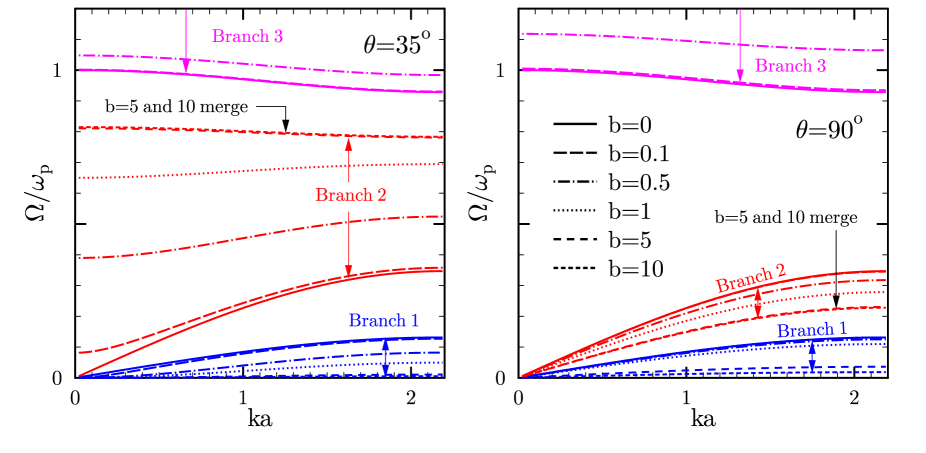
Figure 1: (Color online) Phonon spectrum of the magnetized bcc lattice for several values of $b=\omega_{\rm B}/\omega_{\rm p}$. Magnetic field ${\bm{B}}$ and wavevector ${\bm{k}}$ orientations are defined in the text. Left and right panels correspond to angles between ${\bm{k}}$ and ${\bm{B}}$ of $35^{\circ}$ and $90^{\circ}$, respectively. Branch 3 curves for $b\geq 1$ are not shown. $a=(4\pi n/3)^{-1/3}$ is the ion sphere radius.

In this work we fix the direction of the magnetic field as ${\bm{n}}=(1,1,1)/\sqrt{3}$. This direction coincides with the direction towards one of the nearest neighbors in the bcc lattice. It also corresponds to the minimum of the magnetized bcc crystal zero-point energy (Baiko, 2009). The phonon spectra in the directions of the wavevector ${\bm{k}}/k=(1,1,0)/\sqrt{2}$ and ${\bm{k}}/k=(1,-1,0)/\sqrt{2}$ are shown on the left and right panels of Fig. 1, respectively, for several values of $b$. Left panel corresponds to an angle of about $35^{\circ}$ between ${\bm{k}}$ and ${\bm{B}}$. Right panel is for ${\bm{k}}\perp{\bm{B}}$.

Given the phonon frequencies, the phonon thermodynamic functions in the magnetic field can be calculated using the same general formulas (e.g., Landau & Lifshitz, 1980) as in the field-free case. The phonon free energy (with phonon chemical potential $\mu=0$ and without zero-point contribution) reads

$$F = T\sum_{\bm{k}s}\ln{\left[1-\exp{\left(-\frac{\hbar\Omega_{\bm{k}s}}{T}\right)}\right]}$$ (4)

$$= VT\sum_{s}\int_{\rm BZ}\frac{{\rm d}\bm{k}}{(2\pi)^{3}}\ln{\left[1-\exp{\left(-\frac{\hbar\Omega_{\bm{k}s}}{T}\right)}\right]}~{},$$

where $V$ is the volume, and the integral is over the first Brillouin zone. The phonon internal thermal energy $E$ and heat capacity $C$ are then given by

$$E = F-T\left(\frac{\partial F}{\partial T}\right)_{\mu,V}=\sum_{\bm{k}s}\frac{\hbar\Omega_{\bm{k}s}}{e^{\hbar\Omega_{\bm{k}s}/T}-1}~{},$$ (5)

$$C = -T\left(\frac{\partial^{2}F}{\partial T^{2}}\right)_{\mu,V}=\frac{1}{4T^{2}}\sum_{\bm{k}s}\frac{\hbar^{2}\Omega_{\bm{k}s}^{2}}{{\rm sinh}^{2}(\hbar\Omega_{\bm{k}s}/2T)}~{}.$$ (6)

3 Numerical Integration

For accurate and fast numerical integration over the first BZ we have developed a new integration scheme. The need to do this stemmed from the cylindrical geometry imposed on the system by the magnetic field. The typically used BZ integration scheme (Albers & Gubernatis, 1981; Baiko, 2000; Baiko et al., 2001) takes into account crystal geometry only.

The Brillouin zone of the bcc lattice is a rhombic dodecahedron (convex polyhedron with 12 rhombic faces). It consists of 48 identical primitive domains of the form $k^{x}\geq k^{y}\geq k^{z}\geq 0,~{}k^{x}+k^{y}\leq 2\pi/a_{\rm l}$, where $a_{\rm l}$ is the bcc lattice constant, $na_{\rm l}^{3}=2$. 48 domains are obtained by 6 permutations of Cartesian coordinates in the above inequalities and by reflections of 6 resulting domains with respect to planes $k^{x}=0$, or $k^{y}=0$, or $k^{z}=0$, or any combination of the three for a total of 8 distinct possibilities. Each rhombic face can be split by its diagonals into 4 identical triangles (hereafter primitive triangles) and each of the resulting 48 triangles is a face of the respective primitive domain.

In this paper we calculate thermodynamic functions due to the three branches of the phonon spectrum separately. In the absence of the magnetic field it is sufficient to integrate in Eq. (4) over only one primitive domain as all domains yield identical contributions. In the presence of the field it is no longer so. Moreover, dominant contributions to the thermodynamic functions come from different domains for different phonon branches. For instance, for $k\to 0$ the intermediate branch $\Omega_{2}$ is acoustic ($\Omega_{2}\propto k$) in the ${\bm{k}}\perp{\bm{B}}$ plane and is optic ($\Omega_{2}\to{\rm const}$) outside of this plane with $\Omega_{2}(0)$ increasing with decrease of the angle $\theta$ between ${\bm{k}}$ and ${\bm{B}}$ (cf. Fig. 1). At low temperatures this results in $T^{4}$ dependence of the intermediate branch specific heat with dominant contributions coming from the domains containing the ${\bm{k}}\perp{\bm{B}}$ plane. The lowest branch $\Omega_{1}$ is also acoustic for ${\bm{k}}\perp{\bm{B}}$ but is quadratic in $k$ as $k\to 0$ for other angles between ${\bm{k}}$ and ${\bm{B}}$. This results in $T^{3/2}$ dependence of the specific heat at low temperatures with maximum contributions coming from domains containing ${\bm{k}}\parallel{\bm{B}}$.

The integration over ${\bm{k}}$ proceeds as follows. For every phonon branch we specify a $\theta$-grid ($\theta$ is the angle between ${\bm{k}}$ and ${\bm{B}}$), which is denser at those $\theta$, where the maximum contribution to the thermodynamic functions of the given branch is expected (e.g., around $\theta=\pi/2$ for branch $\Omega_{2}$). For every primitive triangle we specify vertices $A$, $B$, and $C$ corresponding to minimum, intermediate, and maximum angles $\theta_{\rm min}$, $\theta_{\rm int}$, and $\theta_{\rm max}$, respectively. These $\theta$ are added to the $\theta$-grid. For every grid-point $\theta_{i}$ from the segments $[\theta_{\rm min},\theta_{\rm int}]$, $[\theta_{\rm min},\theta_{\rm max}]$, and $[\theta_{\rm int},\theta_{\rm max}]$ we find points on the edges of the primitive triangle $[A,B]$, $[A,C]$, and $[B,C]$, respectively, which are characterized by this $\theta_{i}$. For $\theta_{\rm min}<\theta_{i}<\theta_{\rm max}$ there will be two such points, $P_{i}$ and $Q_{i}$. For two neighboring grid-points $\theta_{i}$ and $\theta_{i+1}$, such that $\theta_{\rm min}<\theta_{i}<\theta_{i+1}<\theta_{\rm max}$, we can define two tetrahedra $OP_{i}Q_{i}P_{i+1}$ and $OP_{i+1}Q_{i+1}Q_{i}$, where $O$ is the origin of the ${\bm{k}}$-space. If one of the grid-points corresponds to a vertex (say, $\theta_{i+1}=\theta_{\rm max}$ corresponds to $C$), we can define only one tetrahedron (in this case $OP_{i}Q_{i}C$).

We then integrate over these tetrahedra using a generalization of the method of Albers & Gubernatis (1981). In particular, to integrate over a tetrahedron $OPQR$ in ${\bm{k}}$-space we switch to variables $\xi$, $\eta$, and $\zeta$: ${\bm{k}}=\xi{\bm{k}}(P)+\xi\eta[{\bm{k}}(Q)-{\bm{k}}(P)]+\xi\eta\zeta[{\bm{k}}(R)-{\bm{k}}(Q)]$, where, for instance, ${\bm{k}}(P)$ is the vector from the origin to the point $P$. The Jacobian for this variable change is $\xi^{2}\eta\det{\{K_{i}^{\alpha}\}}$, where $3\times 3$ matrix $K_{i}^{\alpha}$, $i=1,2,3$, $\alpha=x,y,z$, is defined as $K^{\alpha}_{1}=k^{\alpha}(P)$, $K^{\alpha}_{2}=k^{\alpha}(Q)-k^{\alpha}(P)$, $K^{\alpha}_{3}=k^{\alpha}(R)-k^{\alpha}(Q)$. We integrate over $\xi$, $\eta$, and $\zeta$ from 0 to 1 using 8-point Gauss method. At low $T$, we additionally split the interval $[0,1]$ for $\xi$ into a number of subintervals $[0,\xi_{0}],[\xi_{0},\xi_{0}^{(p-1)/p}],\ldots,[\xi_{0}^{1/p},1]$ with $\xi_{0}=10^{-6}$ and $p\sim 10$.

4 Results

4.1 3-branch thermodynamics

Figure 2: Schematic representation of regions of dimensionless temperatures $t$ and magnetic fields $b$, where thermodynamic quantities have different behavior, for branches 1, 2 and 3 (left, middle, and right panels, respectively). Formulas give asymptotes of partial heat capacities $c_{i}(b,t)$ in these regions. In densely shaded regions (IV and V) magnetic field affects thermodynamics significantly, while in open regions (I and II) it is unimportant. In lightly shaded regions III the field affects only $f_{i}(b,t)$. See text for details.

The Helmholtz free energy $F$, internal thermal energy $E$, and heat capacity $C$ of a magnetized Coulomb crystal can be conveniently presented in the form

$$F=-NTf(b,t),\quad E=NTe(b,t),\quad C=Nc(b,t),$$ (7)

where $N$ is the number of ions; $f(b,t)$, $e(b,t)$, and $c(b,t)$ are dimensionless functions of the dimensionless temperature and magnetic field, $t=T/T_{\mathrm{p}}$ and $b=\omega_{\rm B}/\omega_{\rm p}$.

Table 1: Asymptotic regimes of thermodynamic functions

Branch	Regime	$(b,t)$-range	Type
1	I.1	$b\ll t\ll 1$	PL
1	II.1	$t\gg 1$ at $b\lesssim 1$	SAT
1	III.1	$t\gg 1/b$ at $b\gtrsim 1$	SAT
1	IV.1	$t\ll b$ at $b\lesssim 1$; $t\ll 1/b$ at $b\gtrsim 1$	PL
2	I.2	$b\ll t\ll 1$	PL
2	II.2	$t\gg 1$ at $b\lesssim 1$	SAT
2	III.2	$t\gg 1$ at $b\gtrsim 1$	SAT
2	IV.2	$t\ll b$ at $b\lesssim 1$	PL
2	V.2	$t\ll 1$ at $b\gtrsim 1$	PL
3	I.3	$t\ll 1$ at $b\lesssim 1$	EXP
3	II.3	$t\gg 1$ at $b\lesssim 1$	SAT
3	III.3	$t\gg b$ at $b\gtrsim 1$	SAT
3	IV.3	$t\ll b$ at $b\gtrsim 1$	EXP

The thermodynamic functions can be split into partial contributions corresponding to the three phonon spectrum branches ($i=1,2,3$):

$$f(b,t)=\sum_{i}f_{i}(b,t),\quad e(b,t)=\sum_{i}e_{i}(b,t),$$

$$c(b,t)=\sum_{i}c_{i}(b,t).$$ (8)

These partial contributions describe three thermodynamics, each for a particular branch $i$. The combined thermodynamic quantities must satisfy the Bohr-van Leeuwen theorem, which states that thermodynamic functions of a classic system do not depend on magnetic field. Our system is classic when occupation numbers of $all$ phonon modes are large.

Table 2: Asymptotic behavior of heat capacity fits in PL regimes

Branch $i$	Regime	PL index $\gamma$	Asymptote of $c_{i}(b,t)$
1	I.1	3	$2026\,t^{3}$
1	IV.1	1.5	$31.1(bt)^{3/2}$
2	I.2	3	$486.2\,t^{3}$
2	IV.2	4	$1572t^{4}b^{-1}$
2	V.2	4	$5019t^{4}$

For any given $i$ the functions $f_{i}(b,t)$, $e_{i}(b,t)$, and $c_{i}(b,t)$ are related through [cf. Eqs. (4)–(6)]

$$e_{i}(b,t)=t\,\frac{\partial f_{i}(b,t)}{\partial t},\quad c_{i}(b,t)=\frac{\partial\,te_{i}(b,t)}{\partial t}.$$ (9)

Accordingly, it is sufficient to calculate $f_{i}(b,t)$ to determine the other functions.

Table 3: Asymptotic behavior of free energy fits in SAT regimes

Branch $i$	Regime	Asymptote of $f_{i}(b,t)$
1	II.1	$\ln t+1.392$
1	III.1	$\ln(tb)+1.795$
2	II.2	$\ln t+0.9338$
2	III.2	$\ln t+0.70$
3	II.3	$\ln t+0.168$
3	III.3	$\ln(t/b)$

It is convenient to distinguish different regimes of thermodynamic functions. For a magnetized crystal there are a total of 13 regimes for the three phonon branches. They are realized in different regions of $b$ and $t$ sketched in Fig. 2 and listed in Table 1. These thermodynamic regimes can be divided into low-temperature (quantum) and high-temperature (classic) ones.

In the low-temperature regimes, only a small fraction of phonon modes has non-zero occupation numbers, so that the thermodynamic functions are small [$f_{i}(b,t)\ll 1$, $e_{i}(b,t)\ll 1$, $c_{i}(b,t)\ll 1$]. The low-temperature regimes are further subdivided into those where the thermodynamic functions decrease with decreasing temperature according to a power law or exponentially (PL or EXP regimes in Table 1). In general, we have 5 quantum PL regimes (I, IV, V for branches 1 and 2) and two quantum EXP regimes (I and IV for branch 3 only).

According to Eq. (9), in a PL regime with index $\gamma$ we have

$$c_{i}(b,t)=(\gamma+1)e_{i}(b,t)=(\gamma+1)\gamma f_{i}(b,t)=c_{i0}t^{\gamma},$$ (10)

where $c_{i0}$ is independent of $t$ but may depend on $b$. The specific PL asymptotes of the heat capacity are listed in Table 2. These expressions follow from our fit expressions (Sects. 4.3 and 4.4) and are consistent with our numerical results. We see that in the 5 PL regimes we have $\gamma=$3, 3/2, and 4. The PL regime with $\gamma=3$ (regime I.1 or I.2) is the textbook Debye case of $T^{3}$ dependence of the heat capacity due to acoustic phonons. The PL dependence of magnetized crystal heat capacity with $\gamma=3/2$ (regime IV.1) was predicted by Usov et al. (1980) based on the $k^{2}$ dependence of the branch 1 frequency at small $k$. Similar dependence is obtained for magnon heat capacity (e.g., Kittel, 1995).

The $T^{4}$ regime reported here for branch 2 heat capacity (regimes IV.2 and V.2) stems from the combined dependence of the frequency on $k$ and on the angle $\chi=\pi/2-\theta$ between the wavevector and the plane orthogonal to the magnetic field. The behavior of the frequency $\Omega_{2}$ at small $k$ and $\chi$ can be understood if one reverses signs in front of the square roots in Eq. (14) or (15) of Baiko (2009). In both ways one obtains $\Omega_{2}\approx\omega_{\rm p}\sqrt{|E_{B}|/(1+b^{2})}$, where $E_{B}$ is given by Eq. (12) of the same paper. To lowest order in $k$ and $\chi$, one can then write

$$\hbar\Omega_{2}\approx\sqrt{\alpha^{2}k^{2}+\beta^{2}\chi^{2}}~{},$$ (11)

where coefficients $\alpha^{2}$ and $\beta^{2}$ depend on $b$, on the azimuthal angle $\phi$ of ${\bm{k}}$ with respect to ${\bm{B}}$, and on the direction of ${\bm{B}}$; these coefficients are always positive. Internal energy $E_{2}$ of the second branch phonons can be written as [cf. Eqs. (4) and (5)]

$$\frac{(2\pi)^{3}E_{2}}{V}=\int\frac{\hbar\Omega_{{\bm{k}}2}\,\,{\rm d}{\bm{k}}}{\exp{\left(\hbar\Omega_{{\bm{k}}2}/T\right)}-1}$$

$$=\int_{0}^{2\pi}{\rm d}{\phi}\int^{\pi/2}_{-\pi/2}{\rm d}\chi\cos{\chi}\int\frac{\hbar\Omega_{{\bm{k}}2}k^{2}\,{\rm d}k}{\exp{\left(\hbar\Omega_{{\bm{k}}2}/T\right)}-1}~{}.$$ (12)

In the $T\to 0$ limit one can extend integrations over $k$ and $\chi$ out to infinity, replace $\cos{\chi}$ by 1 and employ Eq. (11). After that, at each $\phi$ one can replace integration variables $(k,\chi)\to(r,s)$, where $\alpha k=r\cos{s}$, $\beta\chi=r\sin{s}$, and $r$ varies from 0 to $\infty$, while $s$ varies from $-\pi/2$ to $\pi/2$. This yields

$$E_{2}=\Phi\int_{-\pi/2}^{\pi/2}{\rm d}s\int_{0}^{\infty}{\rm d}r\,\frac{r^{4}\cos^{2}{s}}{\exp{(r/T)}-1}=12\pi\zeta(5)\Phi T^{5},$$ (13)

where $\Phi$ is a constant determined by the $\phi$-integral. Heat capacity is then proportional to $T^{4}$.

In the high-temperature regimes (denoted as SAT in Table 1), all phonon modes of a given branch are fully excited. Partial internal energy and heat capacity functions $e_{i}$ and $c_{i}$ saturate at their maximum value 1, while free energies reach logarithmic asymptotes:

$$e_{i}(b,t)\to 1,\quad c_{i}(b,t)\to 1,\quad f_{i}(b,t)\to\ln t+F_{i}~{}.$$ (14)

There are 6 classical (SAT) regimes (two regimes, II and III, for each mode). In Eq. (14), $F_{i}$ are temperature-independent but can depend on $b$ (being determined by the logarithm of a phonon frequency, $\ln\Omega_{i}$, averaged over the Brillouin zone). At the same time, $\sum_{i}F_{i}$ is $b$-independent in accordance with the Bohr-van Leeuwen theorem. Values of $F_{i}$ used in our fits are given in Table 3. They are consistent with asymptotes that can be extracted from our numerical data.

Densely shaded ($b,t$)-regions in Fig. 2 show those regimes where all thermodynamic functions (for a given branch) are strongly affected by the magnetic field. These are seen to be quantum regimes IV and V. Lightly shaded regions (regions III for any $i$) indicate the saturation regimes where only $f_{i}(b,t)$ is affected by the magnetic field [through $F_{i}$ in Eq. (14)]. Finally, in blank regions (I and II for any $i$) magnetic field effects are weak.

Table 4: Fit accuracy of thermodynamic functions

Function	$\delta_{\mathrm{rms}}$	$\delta_{\mathrm{max}}$	$b_{m}$	$t_{m}$
$f(0,t)$	0.0022	0.0070	0	0.00501
$e(0,t)$	0.0026	0.0081	0	0.0158
$c(0,t)$	0.0030	0.0105	0	0.0126
$f(b,t)$	0.019	0.106	0.00158	0.000126
$e(b,t)$	0.019	0.113	0.00251	0.000126
$c(b,t)$	0.019	0.117	0.00251	0.000100

4.2 Calculations and fits

Using the technique described in Sect. 3 we have calculated 9 thermodynamic functions $f_{i}(b,t)$, $e_{i}(b,t)$, and $c_{i}(b,t)$ defined by Eqs. (7) and (8). The calculations were done on a dense grid of temperatures (81 $t$-points logarithmically equidistant in the interval from $10^{-4}$ to $10^{4}$). We have considered the non-magnetized crystal ($b=0$) and 31 magnetic field values $b$ (logarithmically equidistant in the range from $10^{-3}$ to $10^{3}$).

The thermodynamic functions vary over many orders of magnitude in a non-trivial manner. To facilitate the use of these results, we have fitted the calculated functions by analytic expressions. The fit formulas are presented and discussed below. Here we outline their general features.

For branches $i=1$ and 2 we fit $f_{i}(b,t)$ by the functions

$$f_{i}(b,t)=\ln\left(1+\frac{P_{i}(b,t)}{Q_{i}(b,t)}\right),$$ (15)

where $P_{i}(b,t)$ and $Q_{i}(b,t)$ are certain sums of power-law functions of $t$.

The cyclotron branch $3$ is different. Its thermodynamics is well described by the Einstein model with some oscillator frequency $\omega=\kappa(b)\,\omega_{\mathrm{p}}$:

$$f_{3}(b,t)=\ln\left(\frac{1}{1-\exp(-\kappa(b)/t)}\right),$$ (16)

where $\kappa(b)$ is temperature independent.

We will present the analytic fit expressions for $f_{i}(b,t)$ only. Other thermodynamic quantities can be calculated from $f_{i}(b,t)$ using Eq. (9). We have verified that the expressions for $e_{i}(b,t)$ and $c_{i}(b,t)$, obtained from our analytic fits to $f_{i}(b,t)$, describe well the calculated values of $e_{i}(b,t)$ and $c_{i}(b,t)$. The asymptotes presented in Tables 2 and 3 correspond to the fit expressions.

Table 4 summarizes the accuracy of our fits. Three upper lines give root-mean-square (rms) relative deviations $\delta_{\mathrm{rms}}$ and maximum deviations $\delta_{\mathrm{max}}$ of the fitted and calculated total thermodynamic functions (summed over all branches) for a non-magnetized crystal ($b=0$). Deviations are determined over all 81 temperature grid points. The fits are seen to be rather accurate, with $\delta_{\mathrm{rms}}\lesssim 0.3\%$ and $\delta_{\mathrm{max}}\lesssim 1\%$. Three last lines list $\delta_{\mathrm{rms}}$ and $\delta_{\mathrm{max}}$ of the total thermodynamic functions for a magnetized crystal (over all $81\times 32=2592$ grid points of $t$ and $b$). These fits are less accurate ($\delta_{\mathrm{rms}}\lesssim 2\%$ and $\delta_{\mathrm{max}}\lesssim 11\%$). The last two columns of Table 4 present the values of $b_{m}$ and $t_{m}$, where the maximum errors occur.

Note that recently Potekhin & Chabrier (2013) have produced analytic fits to thermodynamic functions calculated by Baiko (2000, 2009). Our fit expressions are different. We fit more extended set of more precisely calculated numerical data. In addition, we approximate separately the contributions of different phonon branches while Potekhin & Chabrier (2013) fitted the thermodynamic functions summed over phonon branches. Their fits contain fewer fit parameters but are somewhat less accurate. For instance, comparing those fits with our newly calculated $c(t,b)$ we obtain $\delta_{\mathrm{rms}}\approx 12$%, and $\delta_{\mathrm{max}}\approx 56$% (at $b_{m}=63.096$ and $t_{m}=0.0001$); cf. Table 4.

4.3 Field-free case

Thermodynamics of non-magnetized Coulomb crystals is well studied. The Debye temperature of the crystal can be shown to be $\Theta=0.4532\,T_{\mathrm{p}}$ (Carr, 1961). For all three branches one has two asymptotic regimes, the quantum regime $t\ll 1$, and the classic one $t\gg 1$ (Fig. 2: I and II).

Table 5: Fit parameters in Eqs. (17), (21)–(24)

$\ell$	$a_{1\ell}$	$a_{2\ell}$	$q_{\ell}$	$r_{\ell}$	$\mu_{\ell}$	$\nu_{\ell}$
1	168.83	40.517	2.569	4.503	2.737	1.650
2	0.3317	0.0351	–1.986	4.927	–45100	0.2655
3	122200	4718.4	0.5184	2.3156	25.09	1
4	3.153	1.621	35.73	6.579	0	1
5	316.7	65.82	1.162	1.570	37.15	0.8881
6	3339	335.6	0.4856	2.252	31.26	1
7	30370	1854.6	0.5640	2.335	32.01	1

For branches $i=1$ and 2 we suggest the fits (15) with

$$P_{i}(0,t) = a_{i1}t^{3}+a_{i2}t^{4}+a_{i3}t^{5},$$

$$Q_{i}(0,t) = 1+a_{i4}t+a_{i5}t^{2}+a_{i6}t^{3}+a_{i7}t^{4}.$$ (17)

The fit parameters $a_{i\ell}$ are collected in Table 5. The quantum regimes I.1 and I.2 are the Debye power-law with $\gamma=3$ in (10) due to the excitation of acoustic phonons with frequencies $\Omega_{1,2}\ll\omega_{\mathrm{p}}$.

For the optical branch 3 we have Eq. (16) with

$$\kappa=\kappa(0)=0.8443.$$ (18)

Accordingly, its contribution is exponentially suppressed at $t\ll 1$ in regime I.3 [$f_{3}(0,t)\sim e_{3}(0,t)\sim c_{3}(0,t)\sim\exp(-\kappa/t)\ll 1$], but the saturation regime II.3 is similar to those of the acoustic modes 1 and 2. Strictly speaking, at very low $t\lesssim 0.01$ the calculated thermodynamic quantities for branch 3 start to deviate from the pure Einstein model (16), but they become so small that their contribution to thermodynamics is negligible. Therefore, the use of Eq. (18) for all $t$ is well justified.

The fits (17) and (18) are reasonably accurate (Table 4). Note that more accurate fits to the total functions $f(0,t)$, $e(0,t)$, and $c(0,t)$ are given by Baiko et al. (2001).

Our calculations and fits reproduce (Table 2) the well known low-temperature asymptote (Carr, 1961):

$$c(0,t)=2513\,t^{3}\quad{\rm at}~{}t\ll 1~{},$$ (19)

and the well known high-temperature asymptote (Pollock & Hansen, 1973):

$$f(0,t)=3(\ln t+0.8313)\quad{\rm at}~{}t\gg 1~{}.$$ (20)

4.4 Magnetized crystal

For the free energy function $f_{1}(b,t)$ of the magnetized crystal we suggest the fit (15) with

$$P_{1}= 8.293(bt)^{3/2}+a_{11}\alpha_{1}^{3}t^{3}+a_{12}\alpha_{2}^{4}t^{4}+a_{13}\alpha_{3}^{5}t^{5},$$

$$Q_{1}= 1+a_{14}\alpha_{4}t+a_{15}\alpha_{5}^{2}t^{2}+a_{16}\alpha_{6}^{3}t^{3}+a_{17}\alpha_{7}^{4}t^{4},$$ (21)

where

$$\alpha_{\ell}=\sqrt{1+q_{\ell}b+r_{\ell}b^{2}},$$ (22)

and the fit coefficients $q_{\ell}$ and $r_{\ell}$ are given in Table 5.

This fit incorporates all the asymptotic regimes shown in Fig. 2. In particular, it reduces to (17) in the limit of $b\to 0$; it reproduces thermodynamic function slope change (from $\gamma=3$ to $3/2$) in quantum regime IV as well as the reduction of the branch 1 saturation temperature and the modification of the classic asymptote of $f_{1}$ at $b\gg 1$ in regime III.

For branch 2 we obtain the fit (15) with

$$P_{2} = a_{21}\beta_{1}t^{4}+a_{22}\beta_{2}t^{5}+a_{23}\beta_{3}t^{6},$$

$$Q_{2} = \beta_{*}+\beta_{**}\sqrt{t}+t$$ (23)

$$+ a_{24}\beta_{4}t^{2}+a_{25}\beta_{5}t^{3}+a_{26}\beta_{6}t^{4}+a_{27}\beta_{7}t^{5},$$

where all magnetic field effects are included into the fit coefficients

$$\beta_{\ell} = 1+\frac{\mu_{\ell}\,b^{2}}{\nu_{\ell}+b^{2}},$$ (24)

$$\beta_{*} = 0.5154\left(b^{2}\over 1+b^{2}\right)^{1/2}+0.08791\,\frac{b^{2}}{1+b^{2}},$$

$$\beta_{**} = -0.3527\left(b^{2}\over 1+b^{2}\right)^{1/4}-0.0706\,\frac{b^{2}}{0.2655+b^{2}}.$$ (25)

The fit coefficients $\mu_{\ell}$ and $\nu_{\ell}$ in Eq. (24) are given in Table 5. In the limit $b\to 0$ the coefficients $\beta_{*}$ and $\beta_{**}$ vanish and the ratio $Q_{2}/P_{2}$ given by Eq. (23) reduces to that given by the field-free fit (17). By construction, the fit (23) also reproduces the asymptotes of Fig. 2 including the thermodynamic function slope change from $\gamma=3$ to 4 in quantum regimes IV and V and modification of the classic asymptote of $f_{2}$ at large $b$ in regime III. At $b\gtrsim 1$ thermodynamics of branch 2 becomes independent of $b$ because the spectrum of branch 2 phonons becomes field-independent (cf. Fig. 1). This remarkable property is implanted in our fit (23): all coefficients $\beta_{\ell}$, $\beta_{*}$ and $\beta_{**}$ become $b$-independent at $b\gtrsim 1$.

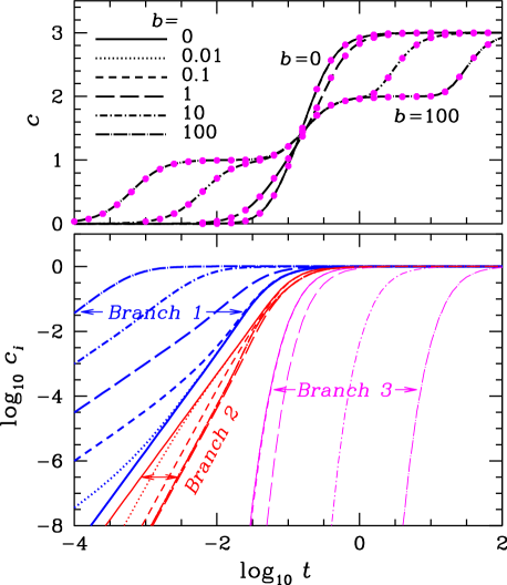
Figure 3: (Color online) Top: Total heat capacity (in linear scale) versus ${\rm log}_{10}t$ for $b=$0, 0.01, 0.1, 1, 10, and 100 (lines of different types are plotted using original calculations; dots are given by the fit expressions at some selected $t$ points). Bottom: Logarithm of partial heat capacities $c_{i}(b,t)$ versus ${\rm log}_{10}t$ at the same $b$. See text for details.

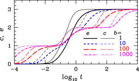
Figure 4: (Color online) Total heat capacity $c(b,t)$ (thin lines) and internal energy $e(b,t)$ (thick lines) versus ${\rm log}_{10}t$ at $b=$1, 10, 100, and 1000 (lines of different types). See text for details.

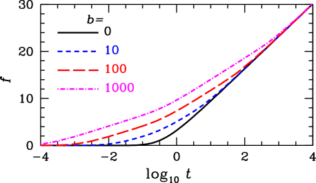
Figure 5: (Color online) Total free energy $f(b,t)$ versus ${\rm log}_{10}t$ at $b=$0, 10, 100, and 1000 (lines of different types). See text for details.

Finally, the branch 3 thermodynamics is well described by the Einstein model of one oscillator with the frequency $\Omega_{3}=\sqrt{(0.8443\,\omega_{\mathrm{p}})^{2}+\omega_{\mathrm{B}}^{2}}$. This implies Eq. (16) with

$$\kappa(b)=\sqrt{0.8443^{2}+b^{2}}~{}.$$ (26)

In the limit of $b\to 0$ this equation reduces to (18). In the limit of $b\gg 1$ we have $\Omega_{3}\to\omega_{\mathrm{B}}$, which yields the thermodynamics due to cyclotron rotation of ions. Again, expression (26) reproduces all asymptotic regimes shown in Fig. 2 and Table 3. Because of the Einstein character of the branch 3 spectrum, thermodynamic functions in quantum regimes I.3 and IV.3 are exponentially suppressed. There are small deviations from the Einstein model in these regimes, but these deviations can be neglected in the total thermodynamic functions.

4.5 Total thermodynamic functions

Thermodynamics of magnetized Coulomb crystals was analyzed by Baiko (2000, 2009). We outline the main properties emphasizing the contribution of different phonon branches into total thermodynamic functions (7). All the curves presented in this section are plotted using calculated data. The fits would give very close curves. To illustrate this point in the upper panel of Fig. 3 we show the fit results for some selected values of $b$ and $t$.

Figure 3 plots the heat capacity. The lower panel shows the partial heat capacities $c_{1}(b,t)$, $c_{2}(b,t)$, and $c_{3}(b,t)$ (on logarithmic scale) versus ${\rm log}_{10}t$ for $b=0$, 0.01, 0.1, 1, 10, and 100. When the magnetic field increases, $c_{1}(b,t)$ grows up. In this way the magnetic field lowers the saturation temperature (at which $c_{1}(b,t)\approx 1$) and the power-law index (from 3 to 3/2) in quantum regime (Table 2). Thus the magnetic field invalidates the Debye $T^{3}$ law; the notion of the Debye temperature cannot be applied to a magnetized Coulomb crystal. At $b\gtrsim 1$ the saturation temperature for branch 1 phonons scales as $1/b$. On the contrary, the same growing magnetic field reduces $c_{2}(b,t)$ and increases the power-law index (from 3 to 4) in quantum regime (Table 2). In this case the magnetic field does not affect the saturation temperature, and the heat capacity $c_{2}(b,t)$ at $b\gtrsim 1$ becomes almost independent of $b$. Accordingly, all curves for $b\geq 1$ in the lower panel of Fig. 3 merge, so that when $b$ varies $c_{2}(b,t)$ actually changes only between the $b=0$ and $b=1$ curves. As for $c_{3}(t,b)$, the magnetic field increases the saturation temperature. At $b\lesssim 1$ the increase is small (and all the curves at $b<1$ almost merge), but at $b\gtrsim 1$ the saturation temperature increases proportional to $b$. Below saturation, $c_{3}(b,t)$ is exponentially small.

The upper panel of Fig. 3 plots the total heat capacity $c(b,t)$ (in natural scale) versus ${\rm log}_{10}t$ for the same $b$. As long as $b\lesssim 1$, the magnetic field affects only the low-temperature part of the $c(b,t)$-curve (which is invisible in the upper panel of Fig. 3 but which would be quite visible in logarithmic scale, as in the lower panel — see the left panel of Fig. 2 in Baiko 2009). A stronger field $b\gtrsim 1$ dramatically changes $c(b,t)$ because of large separation of saturation temperatures in branches 1, 2, and 3. With increasing $t$, branch 1 saturates first at $t\sim 1/b$ and we have $c(b,t)\approx 1$; then branch 2 saturates at $t\sim 1$ after which $c(b,t)\approx 2$, and finally the last branch 3 saturates at $t\sim b$ giving $c(b,t)\to 3$.

Figure 4 compares the temperature dependence of the heat capacity $c(b,t)$ (thin lines) and internal energy $e(b,t)$ (thick lines) for $b=$1, 10, 100, and 1000 (lines of different types). Figure 5 plots the free energy function $f(b,t)$ for $b=$0, 10, 100, and 1000. As long as $b\lesssim 1$, the magnetic field affects only low-temperature ($t\lesssim b$) parts of the curves which are again invisible in natural scale of Figs. 4 and 5 (cf. Figs. 2 and 4 in Baiko 2009). Accordingly, the functions $c(b,t)$, $e(b,t)$, and $f(b,t)$ in our Figs. 4 and 5, if plotted at several values of $b\lesssim 1$, would look almost the same as those at $b=0$. However, at higher $b$ the magnetic field strongly affects these thermodynamic functions. The temperature dependence of $e(b,t)$ is seen to be smoother but similar to that of $c(b,t)$: it reflects the saturation of different phonon branches at different temperatures. Note that at $t\sim 1$ and any $b\gtrsim 1$ all functions $e(b,t)$ practically merge, and so do all functions $c(b,t)$. This is because the behavior of these functions at $t\sim 1$ is determined by the branch 2 frequencies which cease to depend on $b$ at $b\gtrsim 1$. The temperature dependence of $f(b,t)$ is different because the free energy does not saturate but grows logarithmically at classic temperatures.

After all the three phonon branches saturate at sufficiently high temperature, total thermodynamic functions become independent of $b$ and coincide with those at $b=0$. In particular, $f(b,t)$ must be given by the asymptote (20). We have verified that our numerical results are consistent with this expectation (cf. Table 3).

4.6 Zero-point contribution

The Helmholz free energy and the internal energy have the same extra (positive) contribution $(3N/2)\varepsilon_{0}$ due to zero-point ion vibrations. The mode-average oscillator energy $\varepsilon_{0}$ depends on $b$. We can split $\varepsilon_{0}$ into three terms corresponding to different phonon branches, $\varepsilon_{0}=\varepsilon_{1}+\varepsilon_{2}+\varepsilon_{3}$, where $3N\varepsilon_{i}=\sum_{\bm{k}}\hbar\Omega_{\bm{k}i}$, and summation is over the first Brillouin zone. We have calculated $\varepsilon_{i}$ and propose the following analytical expressions to describe the numerical results:

$$\varepsilon_{1} = \frac{0.09005\,\,\hbar\omega_{\rm p}}{\sqrt{1+0.3981b+1.795b^{2}}}~{},$$

$$\frac{\varepsilon_{2}}{\hbar\omega_{\rm p}} = \frac{0.1379}{1+4.542b^{2}}+\frac{0.1804b^{2}}{b^{2}+1/4.542}~{},$$

$$\varepsilon_{3} = \hbar\omega_{\rm p}\sqrt{0.2834^{2}+b^{2}/9}~{}.$$ (27)

The rms errors of these fits are below 1%. Maximum errors are below 2%. At $b=0$ we have $\varepsilon_{0}/\hbar\omega_{\rm p}\approx 0.5114$, which is the well-known moment $u_{1}$ of the bcc lattice (Carr, 1961). At $b\gg 1$ the dominant contribution is due to the third branch: $\varepsilon_{3}\approx\hbar\omega_{\rm B}/3$.

5 Discussion

Figure 6: $T-\rho$ regions at $B=3\times 10^{15}$ G in the neutron star crust composed of ground-state matter where heat capacity of Coulomb crystal has different behavior (Table 6). $T_{\mathrm{m}}$ is the melting temperature; vertical dotted line separates the outer and inner crust. In the singly-shaded region the $B$-field effects are unimportant, while in the doubly-shaded region they affect the heat capacity. See text for details.

Table 6: Asymptotic behavior of total crystal heat capacity per one ion in different $T-\rho$ regions shown in Fig. 6

Regime	Dominant branch	$B$-field effect	Asymptote of $c$
C3	1,2,3	absent	3
C2	1,2	present	2
C1	1	present	1
Q0	1,2	absent	$2513\,t^{3}$
QB	1	strong	$31\,(bt)^{3/2}$

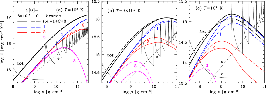
Figure 7: (Color online) Specific heat capacity (at constant volume per cubic centimeter) versus density in the outer crust of a neutron star for $B=3\times 10^{15}$ G (solid lines) and $B=0$ (dashed lines). Three panels (a), (b), and (c) are for $T=10^{8}$, $3\times 10^{7}$, and $10^{7}$ K, respectively. Medium-width lines 1, 2, and 3 show partial crystal heat capacities due to respective phonon branches. Thick lines tot are total crystal heat capacities. Thin lines e are electron heat capacities. See text for details.

In this section we apply the analytical formulas of Sect. 4 to study the heat capacity of the magnetized crystalline neutron star crust. The temperature-density diagram of the crust with $B=3\times 10^{15}$ G is plotted in Fig. 6. We assume the ground-state composition of the crust and use the simplified smooth-composition model (Haensel, Potekhin & Yakovlev, 2007). The same diagram for the accreted crust composition (e.g., Haensel, Potekhin & Yakovlev 2007) should be qualitatively similar. For simplicity, we neglect magnetic field effects on the nuclear composition of the crust.

The dotted vertical line in Fig. 6 shows the neutron drip point ($\rho_{\mathrm{ND}}\approx 4.3\times 10^{11}$ g cm^-3). It separates the outer and inner crust. The outer crust consists of electrons and ions; the latter are fully ionized by the electron pressure for rather high densities displayed in the figure. The inner crust consists of electrons, ions and free neutrons. The inner crust extends to the density $\approx 1.5\times 10^{14}$ g cm^-3. We do not display the highest-density inner crust because its composition is not very certain (may contain funny pasta phases of nuclear clusters, as reviewed, for instance, by Haensel, Potekhin & Yakovlev 2007).

The upper line in Fig. 6 is the melting temperature $T_{\rm m}$ of the field-free crystal. Our analysis is thus limited to the shaded region below $T_{\rm m}$. Various other lines in Fig. 6 split the $T-\rho$ plane into several domains ($C1$, $C2$, $C3$, $Q0$, and $QB$), where the ion heat capacity shows qualitatively different behavior at $B=3\times 10^{15}$ G. These regimes are listed in Table 6. Notice that the boundaries between the domains are approximate and the change of heat capacity when moving from one domain to another is smooth.

The line $T_{\mathrm{B}}$ is the ion cyclotron temperature (defined as $T_{\mathrm{B}}=\hbar\omega_{\mathrm{B}}$ and expressed in Kelvins). At $T>T_{\mathrm{B}}$ the magnetic field has almost no effect on the heat capacity of ions (domains $C3$ and $Q0$). In the doubly-shaded region $T<T_{\mathrm{B}}$ (domains $C2$, $C1$, and $QB$) the magnetic field affects the ion heat capacity. For $B=3\times 10^{15}$ G the ion heat capacity of the crust is thus affected as long as $T\lesssim 10^{8}$ K. Straightforward scaling implies that the field $B\sim 3\times 10^{14}$ G becomes important at $T\lesssim 10^{7}$ K, while $B\sim 3\times 10^{16}$ G modifies the ion heat capacity at $T\lesssim 10^{9}$ K.

The temperature $T_{\mathrm{p}}^{*}$ in Fig. 6 is defined as $T_{\mathrm{p}}^{*}=0.1\,T_{\mathrm{p}}$. It is a better measure of quantum effects in a $B=0$ Coulomb crystal than $T_{\mathrm{p}}$ itself. We also plot the temperature $T_{\mathrm{q}}=T_{\mathrm{p}}^{*2}/T_{\mathrm{B}}$ (at those mass densities $\rho$, where $T_{\mathrm{q}}<T_{\mathrm{p}}^{*}$). As $B$ increases, this line shifts to the right ($T_{\mathrm{q}}$ becomes lower at given $\rho$).

Domain $C3$ in Fig. 6 corresponds to classic (high-temperature) crystal where all the three phonon branches are saturated and the magnetic field does not affect the heat capacity ($c\approx 3$, Table 6). In domain $C2$ the magnetic field reduces the contribution of phonon branch 3, but branches 1 and 2 are still saturated ($c\approx 2$). In domain $C1$ the magnetic field reduces the contribution of phonon branch 2 although branch 1 remains saturated ($c\approx 1$). When $T$ falls below $T_{\mathrm{q}}$ one enters domain $QB$, which corresponds to quantum power law regime IV.1 of Fig. 2. All phonon branches are non-saturated, and the leading heat capacity $\propto T^{3/2}$ is produced by branch 1. The magnetic field effect is the strongest in this regime. The variation of the heat capacity in these movings ($C3\to C2\to C1\to QB$) can be easily understood from Fig. 3. At $T_{\mathrm{p}}^{*}>T>T_{\mathrm{B}}$ (domain $Q0$) one has a quantum crystal unaffected by magnetic field. The ion heat capacity there is $\propto T^{3}$ and is due to phonon branches 1 and 2 (regimes I.1 and I.2 in Fig. 2).

Let us mention that for any value of $B$ from $\sim 10^{14}$ G to $\sim 3\times 10^{16}$ G, one can estimate the ion heat capacity in the crust by rescaling the lines $T_{\mathrm{B}}$ and $T_{\mathrm{q}}$ in Fig. 6. At $B\lesssim 10^{14}$ G the temperature $T_{\mathrm{B}}$ becomes lower than $T_{\mathrm{p}}^{*}$ and at $B\gtrsim 3\times 10^{16}$ G it becomes higher than $T_{\mathrm{p}}^{*}$ in the entire density range displayed, and some domains move out of the picture.

The above discussion is further illustrated in Fig. 7. It compares ion and electron heat capacities (at constant volume per cubic centimeter) as functions of density in the outer neutron star crust. Three panels (a), (b), and (c) are for $T=10^{8}$, $3\times 10^{7}$ and $10^{7}$ K, respectively. Solid and dashed lines represent heat capacities at $B=3\times 10^{15}$ G and at $B=0$. Thick lines (labeled as tot) plot the total ion heat capacity (sum over three phonon branches). Medium-thick lines (labeled as 1, 2, and 3) display the partial contributions of phonon branches 1, 2, and 3, respectively. Finally, thin lines (denoted as $e$) present the electron heat capacities. The electron heat capacity in a magnetic field (thin solid line) oscillates with growing density because degenerate electrons populate new Landau levels. With decrease of temperature, the oscillations become more pronounced. Comparing the ion and electron heat capacities in Fig. 7, we conclude that the ion heat capacity, for the most part, dominates in the outer crust for the given temperature range.

The behavior of the ion heat capacity in Fig. 7 is easily understood from Fig. 6. The temperature $T=10^{8}$ K in Fig. 7(a) is close to $T_{\mathrm{B}}$. Accordingly, the field $B=3\times 10^{15}$ G affects the ion heat capacities provided by all phonon branches 1, 2 and 3 only weakly (so that ion solid and dashed lines almost merge). A visible reduction of these heat capacities at higher $\rho$ is explained by the transition from classic to quantum ion crystal. With the drop of $T$ [in Figs. 7(b) and (c)] the effect of the magnetic field on the ion heat capacity becomes stronger. Quantum suppression of the ion heat capacity also grows stronger. These results are in accord with Fig. 6. For instance, the phonon branch 3 contribution at $B=3\times 10^{15}$ G and $T=10^{7}$ in Fig. 7(c) is so small that it is not shown in the figure.

Summarizing, one can say that magnetic field $B\sim 3\times 10^{15}$ G may have an important effect on the ion heat capacity in the outer crust. The ion heat capacity in the inner crust will be also modified by such magnetic field but it will happen at those temperatures where the electron heat capacity dominates [cf. Fig. 7(c)]. For lower $B$, the magnetic field affects the ion heat capacity in smaller ranges of $T$ and $\rho$ in the outer crust.

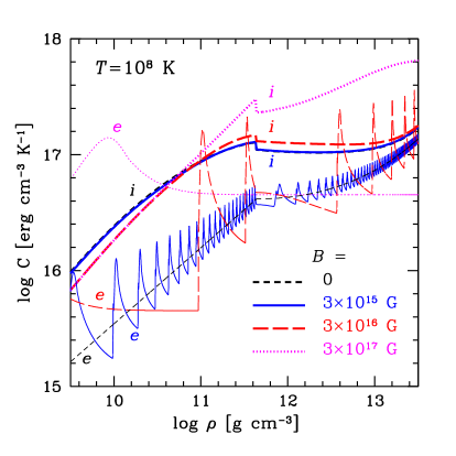
Figure 8: (Color online) The total ion (thick lines $i$) and electron (thin lines $e$) heat capacities for $T=10^{8}$ K versus density in the outer and inner neutron star crust at $B=0$ (short dashes), $3\times 10^{15}$ G (solid lines), $3\times 10^{16}$ G (long dashes) and $3\times 10^{17}$ G (dotted lines).

Larger fields $B>3\times 10^{15}$ G can influence the ion heat capacity in the outer and inner crust at higher $T\gtrsim 10^{8}$ K. To illustrate this statement, in Fig. 8 we plot the total ion (thick lines) and electron (thin lines) heat capacities for $T=10^{8}$ K versus density in the outer and inner crust at $B=0$ (short-dashed lines) and three values of $B$, $3\times 10^{15}$ G (solid lines), $3\times 10^{16}$ G (long-dashed lines), and $3\times 10^{17}$ G (dotted lines). The lines for $B=0$ and $3\times 10^{15}$ G are essentially the same as in Fig. 7(a), but now they are extended to the inner crust. Some jumps of the ion heat capacity occur at the neutron drip point. We see that the field $B\gtrsim 3\times 10^{16}$ G, indeed, noticeably enhances the ion heat capacity in the inner crust, and this contribution will dominate over the electron one. Note a delay of quantum oscillations of the electron heat capacity after the neutron drip point (at $\rho\gtrsim\rho_{\mathrm{NB}}$, $B=3\times 10^{15}$ and $3\times 10^{16}$ G). It is due to the efficient neutronization of matter which is accompanied by a slower growth of the electron number density (and of the electron chemical potential that regulates the quantum oscillations) with increasing $\rho$. The quantum oscillations just after the neutron drip are very sensitive to the density dependence of the electron number density.

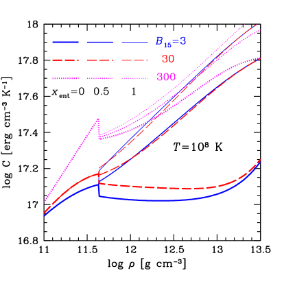
Figure 9: (Color online) The total ion heat capacity for $T=10^{8}$ K versus density in the neutron star crust at $B=3\times 10^{15}$ G (solid lines), $3\times 10^{16}$ G (long dashes) and $3\times 10^{17}$ G (dotted lines). Thick lines correspond to the standard ground state matter; thinner lines are for the matter where one halve of free neutrons are entrained to the nuclei; even thinner lines – all neutrons are entrained (see text for details).

An order of magnitude higher magnetic field $B=3\times 10^{17}$ G would exert the most drastic influence on the ion heat capacity of the entire inner crust of a neutron star. Under conditions shown in Fig. 8 the ion heat capacity at $B=3\times 10^{17}$ G exceeds the field-free value by up to a factor of 4. The reason for this behavior can be traced back to Fig. 3, where the branch 1 heat capacity of a quantum crystal is seen to be greatly amplified by the magnetic field. The strongest effect may be expected at temperatures $T\lesssim 0.1T_{\rm p}^{*}$ (Fig. 6), that is at $T\lesssim 0.01T_{\rm p}\approx 6\times 10^{7}Z_{40}\sqrt{\rho_{14}X/4}/A_{1e3}$ K, combined with $b\gtrsim 1$ or $B\gtrsim 5\times 10^{17}\sqrt{4\rho_{14}/X}$ G. In this case $\rho_{14}$ is the mass density in units of $10^{14}$ g cm^-3, $Z_{40}=Z/40$, $A_{1e3}=A/1000$, where $A$ is the number of nucleons per one nucleus (including free neutrons in the inner neutron star crust), and $X=A/A_{\rm N}$, where $A_{\rm N}$ is the number of nucleons bound in a nucleus ($A_{\rm N}$ determines ion plasma and cyclotron frequencies).

The field $B=3\times 10^{17}$ G is so large that plasma electrons occupy the ground Landau level throughout the whole crust. The heat capacity (per cm³) of relativistic degenerate electrons is then independent of the electron number density (and hence independent of $\rho$). The quantum oscillations of the electron heat capacity are absent. The bump of the electron heat capacity at $\rho\sim 10^{10}$ is caused by the onset of electron degeneracy.

Let us remark that the heat capacity in the inner crust contains also the contribution of free neutrons (omitted in this work). For non-superfluid neutrons, this contribution would dominate. However, it is strongly suppressed and becomes small if neutrons are superfluid (e.g., Gnedin et al., 2001).

Finally, Fig. 9 illustrates the effects of neutron entrainment in the inner crust on the heat capacity of ions. It shows the total ion heat capacity versus density at $T=10^{8}$ K for the same values of $B=3\times 10^{15}$, $3\times 10^{16}$ and $3\times 10^{17}$ G as in Fig. 8 (solid, dashed and dotted lines, respectively). The thick lines are for the same standard model of the inner crust as in Fig. 8. Thinner lines take into account recent theoretical predictions (e.g., Chamel, Page & Reddy 2013, Chamel 2013) that some fraction of free neutrons can be actually entrained by the atomic nuclei. We have incorporated this effect in a schematic manner by increasing masses of atomic nuclei in the inner crust. This reduces the ion plasma and cyclotron frequencies and the suppression of the heat capacity in the quantum regime. The medium size lines are calculated assuming that one half of the free neutrons are entrained in this way ($x_{ent}=0.5$), while the thinnest lines assume that all free neutrons are entrained ($x_{ent}=1$). We see that the entrainment effect can strongly enhance the ion heat capacity in the inner crust.

The present results are important for modeling the structure, evolution and observational manifestations of neutron stars with strong crustal magnetic fields such as magnetars (SGRs and AXPs) and high magnetic field pulsars (Sect. 1). These objects are observationally linked to a wide range of exciting astrophysical phenomena. The internal crustal magnetic fields of these objects are thought to have both, poloidal and toroidal, components ($B_{\mathrm{p}}$ and $B_{\mathrm{tor}}$), and both components can be substantial, especially in the beginning of neutron star lives. For instance, Pons & Perna (2011) simulated the magneto-thermal evolution of the magnetar (AXP) 1E 2259+586 assuming the initial magnetic field values $B_{p}=2.5\times 10^{14}$ G and $B_{\mathrm{tor}}=2.5\times 10^{16}$ G. Our results should help modeling magnetars, high-$B$ pulsars, and their possible mutual transformations (Sect. 1). Primarily, we mean modeling thermo-magnetic evolution of these objects, dynamics of giant and ordinary bursts in magnetars and afterburst relaxation.

6 Conclusions

We have performed accurate calculations of the phonon thermodynamic functions of the magnetized bcc Coulomb crystal and approximated our numerical results by analytic expressions. Thermodynamic properties are fully determined by the free energy function $f(b,t)$ of dimensionless temperature $t$ and magnetic field $b$ [see Eqs. (7) and (8)] which we split into three functions $f(b,t)=f_{1}(b,t)+f_{2}(b,t)+f_{3}(b,t)$ for the three phonon branches. We have derived three fit expressions (21), (23), and (26) for the partial functions $f_{i}(b,t)$. For a non-magnetized crystal the partial functions $f_{i}(0,t)$ are given by simpler fit expressions (17) and (18). Our analytic fits are sufficiently simple for differentiating and obtaining other thermodynamic functions without any significant loss of accuracy (Table 4). In this way we derive selfconsistent analytic description of harmonic-lattice thermodynamics. A similar (simpler but less accurate) description has been obtained earlier by Potekhin & Chabrier (2013). Although our calculations have been performed for restricted values of $t$ and $b$ ($10^{-4}\leq t\leq 10^{4}$; $b=0$ and $10^{-3}\leq b\leq 10^{3}$) we expect that the analytic fits remain accurate for wider ranges of $t$ and $b$. We have also analyzed various behaviors of the thermodynamic functions (Tables 1–3) which may be used for estimating these functions under specific conditions. The results are obtained for one specific orientation of the magnetic field in the crystal but the dependence of thermodynamic functions on the orientation is weak (Baiko, 2000, 2009) and is thus unimportant for many applications.

In addition, we have analyzed (Sect. 5) the behavior of the heat capacity of crystallized ions in the crust of a strongly magnetized neutron star. We have compared the ion heat capacity with the electron one. We have shown that the field $B\lesssim 3\times 10^{15}$ G affects the ion heat capacity in the outer crust at $T\lesssim 10^{8}$ K; in this case the ion heat capacity mainly dominates over the electron one. Stronger $B$-fields can affect the ion heat capacity both in the inner and outer crusts and at higher $T$. Moreover, we have demonstrated that the ion heat capacity in the inner crust is sensitive to the effect of free neutron entrainment by atomic nuclei (Chamel, Page & Reddy 2013, Chamel 2013). We believe that our results will be helpful for modeling observational manifestations of magnetars and high magnetic field pulsars.

References

- Albers & Gubernatis (1981) Albers R.C., Gubernatis J.E., 1981, Los Alamos Scientific Laboratory Report No. LA-8674-MS
- Baiko (2000) Baiko D.A., 2000, PhD thesis, A.F. Ioffe Physical-Technical Institute
- Baiko et al. (2001) Baiko D.A., Potekhin A.Y., Yakovlev D.G., 2001, Phys. Rev. E, 64, 057402
- Baiko (2009) Baiko D.A., 2009, Phys. Rev. E, 80, 046405
- Carr (1961) Carr W.J., 1961, Phys. Rev., 122, 1437
- Chamel (2013) Chamel N., 2013, Phys. Rev. Lett. 110, 011101
- Chamel, Page & Reddy (2013) Chamel N., Page D., Reddy S., 2013, Phys. Rev. C 87, 035803
- Dubin & O’Neil (1999) Dubin D. H. E., O’Neil T. M., 1999, Rev. Mod. Phys. 71, 87
- Gnedin et al. (2001) Gnedin O.Y., Yakovlev D.G., Potekhin A.Y., 2001, MNRAS, 324, 725
- Haensel, Potekhin & Yakovlev (2007) Haensel P., Potekhin A.Y., Yakovlev D.G., 2007, Neutron Stars 1: Equation of State and Structure. Springer, New York
- Itano et al. (1998) Itano W. M., Bollinger J. J., Tan J. N., Jelenkovic B., Huang X.-P., and Wineland D. J., 1998, Science 279, 686
- Kittel (1995) Kittel C., 1995, Introduction to Solid State Physics, 7th edition. Wiley
- Landau & Lifshitz (1980) Landau L.D., Lifshitz E.M., 1980, Statistical Physics. Part I. Pergamon Press, Oxford
- Livingstone et al. (2011) Livingstone M. A., Ng C.-Y., Kaspi V. M., Gavriil F. P., Gotthelf E. V., 2011, Astrophys. J. 730, 66
- Mereghetti (2008) Mereghetti S., 2008, Annual Rev. Astron. Astrophys. 15, 225
- Nagai & Fukuyama (1982) Nagai T., Fukuyama H., 1982, J. Phys. Soc. Jap., 51, 3431
- Nagai & Fukuyama (1983) Nagai T., Fukuyama H., 1983, J. Phys. Soc. Jap., 52, 44
- Pollock & Hansen (1973) Pollock E.L., Hansen J.P., 1973, Phys. Rev. A, 8, 3110
- Pons et al. (2009) Pons J. A., Miralles J. A., Geppert U., 2009, Astron. Astrophys. 496, 207
- Pons & Perna (2011) Pons J. A., Perna R., 2011, Astrophys. J. 741, 123
- Potekhin & Chabrier (2013) Potekhin A. J., Chabrier G., 2013, Astron. Astrophys. 550, A43
- Usov et al. (1980) Usov N.A., Grebenschikov Yu.B., Ulinich F.R., 1980, J. Exp. Theor. Phys. 78, 296
- Woods & Thompson (2006) Woods P.M., Thompson C., 2006, in: Compact stellar X-ray sources, eds. W. Lewin and M. van der Klis, Cambridge University Press, Cambridge
- Zhu et al. (2011) Zhu W. W., Kaspi V. M., McLaughlin M. A., Pavlov G. G., Ng C.-Y., Manchester R. N., Gaensler B. M., Woods P. M., 2011, Astrophys. J. 734, 44