Multicoloring of cannonball graphs

Abstract

The frequency allocation problem that appeared in the design of cellular telephone networks can be regarded as a multicoloring problem on a weighted hexagonal graph, which opened some still interesting mathematical problems. We generalize the multicoloring problem into higher dimension and present the first approximation algorithms for multicoloring of so called cannonball graphs.

1 Introduction

A fundamental problem that appeared in the design of cellular networks is to assign sets of frequencies to transmitters in order to avoid the unacceptable interferences. The number of frequencies demanded at a transmitter may vary between transmitters. The problem appeared in the sixties and was soon related to graph multicoloring problem (see the early survey [4]). It received an enormous attention in the nineties and is still of considerable interest (see [1] and the references there). Besides the mobile telephony there are several applications of frequency assignment including radio and television broadcasting, military applications, satellite communication and wireless LAN [1]. A sizable part of theoretical studies is concentrated on the simplified model when the underlying graph which has to be multicolored is a subgraph of triangular grid (see [10, 11, 4]). This is a natural choice because it is well known that hexagonal cells provide a coverage with the optimal ratio of the distance between centers compared to the area covered by each cell. Such graphs are called hexagonal graphs [16, 17, 19]. Indeed, the model is a reasonable approximation for the rural cellular networks where the underlying graph is often nearly planar, and a popular example are the sets of benchmark problems based on the real cellular network around Philadelphia [2] (see the FAP website [27]). Although the multicoloring of hexagonal graphs seems to be a very simplified optimization problem, some interesting mathematical questions were asked at the time that are still open. An example is the conjecture of McDiarmid and Reed saying that the multichromatic number (the formal definition is given on page 1) of any hexagonal graph $G$ is between $\omega(G)$ and $9\omega(G)/8$, where $\omega(G)$ is the weighted clique number [10]. On the other hand, the hexagonal graph model is known to be practically useless in urban areas, where high concrete buildings on one hand prevent propagation of the radio signals and on the other hand allow very high concentration of users. Loosely speaking, a three dimensional model may be needed in contrast to the hexagonal graphs that are a good model for two dimensional networks. In this paper we discuss a generalization of the multicoloring problem on hexagonal graphs from planar case to three dimensions. It is well known that hexagonal cells of the same size with centers positioned in the triangular grid provide an optimal coverage of the plane. Optimality here means the best ratio between the diameter and the area covered by the cell. The situation is much more interesting in three dimensions. Obviously, optimal cells would be nearly balls, and the question is how to position the centers of the balls to achieve the optimal diameter to the volume ratio. The famous Kepler conjecture was a longstanding conjecture about the ball packing in three-dimensional Euclidean space. It says that no arrangement of equally sized balls filling space has greater average density than that of the cubic close packing (face-centered cubic) and the hexagonal close packing arrangements. The density of these arrangements is slightly greater than 74%. It may be interesting to note that the solution of Kepler’s conjecture is included as a part of 18th problem in the famous Hilbert’s problem list back in 1900 [20]. Recently Thomas Hales, following an approach suggested by Fejes Toth, published a proof of the Kepler conjecture. For more details, see [5, 6]. Given an optimal arrangement of balls, we define a graph by taking the balls (or centers of balls) as vertices and connect each pair of touching balls with an edge. Nonnegative demands are assigned to each vertex and we are interested in multicoloring of the graph induced on vertices of positive demand. Loosely speaking, we generalize the problem of multicoloring of hexagonal graphs from two dimensions to three dimensions. The question has been asked at the Oberwolfach seminar Algorithmische Graphentheorie [26] and we are not aware of any result since then.

More formally, we are interested in multicoloring of weighted graphs $G=(V(G),E(G),d)$, where $V=V(G)$ is the set of vertices, $E=E(G)$ is the set of edges, and $d$ assigns a positive integer $d(v)$ to vertex $v\in V$. $d(v)$ is the weight of a vertex, here also called demand. Adjacent vertices are called neighbors. The degree of a vertex, $deg_{G}(v)=deg(v)$ is the number of neighbors of $v$. A proper multicoloring of $G$ is a mapping $f$ from $V(G)$ to subsets of integers such that $\left|f(v)\right|\geq d(v)$ for any vertex $v\in V(G)$ and $f(v)\cap f(u)=\emptyset$ for any pair of adjacent vertices $u$ and $v$ in the graph $G$. The minimal cardinality of a proper multicoloring of $G$, $\chi_{m}(G)$, is called the multichromatic number. Another invariant of interest in this context is the (weighted) clique number, $\omega(G)$, defined as follows: The weight of a clique of $G$ is the sum of demands on its vertices and $\omega(G)$ is the maximal clique weight on $G$. Clearly, ${\chi}_{m}(G)\geq\omega(G)$. Hexagonal graph is the graph induced on vertices of triangular grid of positive demand. Or, in other words, cells of hexagonal grid are assigned integer demands, and the graph is composed by taking cells as vertices and two hexagons sharing an edge are regarded to be adjacent. In 3-dimensional case we will consider optimal arrangements of balls, and define a graph by taking balls (with positive demand) as vertices, and connect touching balls by edges. We call these graphs the cannonball graphs as Keplers motivation for studying the arrangements of balls was optimal arrangement of cannonballs. In the last decade there were several results on upper bounds for the multichromatic number in terms of weighted clique number for hexagonal graphs, some of which also provide approximation algorithms that are fully distributed and run in constant time [7, 8, 9, 10, 11, 12, 14, 16, 17, 18, 13, 19, 21, 22, 23, 25]. The best known approximation ratios are ${\chi}_{m}(G)\leq(4/3)\omega(G)+O(1)$ in general [10, 12, 16] and ${\chi}_{m}(G)\leq(7/6)\omega(G)+O(1)$ for triangle free hexagonal graphs [7, 13, 14]. The conjecture of McDiarmid and Reed: ${\chi}_{m}(G)\leq(9/8)\omega(G)+O(1)$ remains an open problem [10].

No approximation algorithm and no upper bound was previously known for the multichromatic number of cannonball graphs. Here we give two upper bounds, where the first is easily implied by known results for hexagonal graphs (because a layer in a cannonball graph is a hexagonal graph) and the second is an improvement of the first upper bound using some structural properties of the cannonball graphs. In both cases, constructions are given thus providing polynomial approximation algorithms. The main result of this paper that gives the first answer to the problem asked in [26] is

Theorem 1.1

There is an approximation algorithm for multicoloring cannonball graphs which uses at most $\frac{11}{6}\omega(G)+O(1)$ colors. Time complexity of the algorithm is polynomial.

The paper is organized as follows. In the next section we formally define some basic terminology. In Section 3, we present an overview of the algorithm, while in Section 4 we provide a proof of Theorem 1.1. In the last Section we give some ideas for futher work.

2 Hexagonal and cannonball graphs

First we formally define hexagonal and cannonball graphs. Recall the formal definition of hexagonal graphs: the position of each vertex is an integer linear combination $x\vec{p}+y\vec{q}$ of two vectors $\vec{p}=(1,0)$ and $\vec{q}=(\frac{1}{2},\frac{\sqrt{3}}{2})$ and the vertices of the triangular grid are identified with pairs $(x,y)$ of integers. Put an edge connecting two vertices if the points representing the vertices are at distance one in the triangular grid (in other words, when the corresponding hexagonal cells are adjacent). To construct a hexagonal graph $G$, positive weights are assigned to a finite subset of points in the grid and $G$ is a subgraph induced on $V(G)$, the set of grid vertices with positive weights. Cannonball graphs are constructed in a similar way. However, we have many possibilities already when constructing the underlying grid, which, loosely speaking, consists of tetrahedrons and will be called tetrahedron grid $T$. Optimal arrangement of balls in one layer is to put the centers of balls in the points of triangular grid. Then, there are exactly two possibilities to put a second layer on the top of the first layer. These two arrangements are obviously symmetric, however, when choosing a position for the third layer, there are two possibilities that give rise to different arrangements. We will call them layer-arrangement (a) and layer-arrangement (b), respectively (see figure 1).

Figure 1: Two different arrangements of the third layer.

Consequently, we have an infinite number of tetrahedron grids, that all came from the optimal ball arrangements. One of the arrangements, called the cubic close packing (see case (a) of figure 1), can be described nicely by introducing a third vector $\vec{r}=(\frac{1}{2},\frac{\sqrt{3}}{6},\frac{\sqrt{6}}{3})$ in addition to $\vec{p}=(1,0,0)$ and $\vec{q}=(\frac{1}{2},\frac{\sqrt{3}}{2},0)$. Now the position of each vertex is an integer linear combination $x\vec{p}+y\vec{q}+z\vec{r}$ and the vertices of the triangular grid may be identified with triplets $(x,y,z)$ of integers. Given the vertex $v$, we will refer to its coordinates as $x(v)$, $y(v)$ and $z(v)$, or shortly $x$, $y$, and $z$, when there is no confusion possible. For other arrangements there is no such easy extension of the notation from hexagonal graphs. A cannonball graph $G$ is obtained by assigning integer weights to the points of the tetrahedron grid $T$, taking as $V(G)$ the vertices in the grid with positive weights, and introducing edges between vertices at euclidean distance one (in other words, connecting the touching balls). The cannonball graphs based on the cubic close packing will be called regular cannonball graphs. Clearly, from the construction it follows that any layer of a cannonball graph is a hexagonal graph (maybe not connected).

Formally, a cannonball graph is a graph induced on vertices of positive weight.

There is a natural basic 4-coloring of (unweighted) cannonball graph. Start with any layer and call it the base layer. Introduce coordinates $(x,y,0)$ in this layer and define the base coloring by the formula

$$bc(v)=x\bmod 2+2(y\bmod 2).$$ (1)

Colors of vertices of the next layers are then determined exactly as follows. It is obvious that whenever we store a new layer above (or under) the previous one with fixed coloring, we know that each ball from the new layer is connected to exactly three balls from the previous layer, and all of those balls have different colors. Thus there is exactly one extension of the four coloring to the next layer (see figure s 1 and 2, where 4-coloring, using colors $0,1,2,3$, is presented). It is easy to see that this rule, starting from (1), gives a proper coloring of the next layers. In regular cannonball graphs this coloring can be given by closed expression in the following way:

$$bc(v)=((z+1)\bmod 2)(x\bmod 2+2(y\bmod 2))+(z\bmod 2)((x+1)\bmod 2+2((y+1)\bmod 2)).$$ (2)

From the construction of cannonball graphs it is clear that each vertex has (at most) 6 neighbors in its layer, and in addition (at most) three neighbors in each of the neighboring layers. The degree of a vertex in cannonball graph is hence at most 12 (see figure 2).

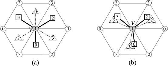
Figure 2: All possible 12 neighbors of vertex $v\in G$ for arrangements (a) and (b). Circles and gray lines represent the middle layer containing $v$, squares and thick lines represent the upper layer, dashed triangles and dashed lines represent the lower layer.

The cliques in the cannonball graphs can have at most four vertices. The (weighted) clique number, $\omega(G)$, is the maximal clique weight on $G$, where the weight of a clique is the sum of weights on its vertices. As cliques in cannonball graphs can have at most four vertices, the weighted clique number is the maximum weight over weights of all tetrahedrons, triangles, edges and weights of isolated vertices. Therefore, we can define invariants $\omega_{i}(G)$ which denote the maximal weight of clique of size at most $i$ on $G$. In fact, we can regard the clique numbers as based on the complete subgraphs of the grid graph because the vertices of weight 0 clearly do not contribute to the clique weights. For example, $\omega_{2}(G)$ is the maximal weight over all edges and isolated vertices. Clearly, for cannonball graphs we have

$$\omega_{1}(G)\leq\omega_{2}(G)\leq\omega_{3}(G)\leq\omega_{4}(G)=\omega(G).$$

An induced subgraph of the cannonball graph without 3-clique will be called a triangle-free cannonball graph.

In the algorithm we will consider some subgraphs of the cannonball graph, in particular, it may be useful to have bipartite subgraphs and 3-colorable subgraph s.

In [10] it was proved that for any weighted bipartite graph $H$, $\chi_{m}(H)=\omega(H)$. Bipartite graph $H$ can be optimally multicolored by the following procedure:

Procedure 2.1

[15] Let $H=(V^{\prime},V^{\prime\prime},E,d)$ be a weighted bipartite graph. We get an optimal multicoloring of $H$ if to each vertex $v\in V^{\prime}$ we assign a set of colors $\{1,2,\ldots,d(v)\}$, while with each vertex $v\in V^{\prime\prime}$ we associate a set of colors $\{m(v)+1,m(v)+2,\dots,m(v)+d(v)\}$, where $m(v)=\max\{d(u):\{u,v\}\in E\}$.

For 3-colorable graphs, there is a simple $\frac{3}{2}$-approximation coloring algorithm.

Lemma 2.1

[19] Every 3-colorable graph can be multicolored using at most $\frac{3}{2}\omega(G)+O(1)$ colors.

Using the proof of Lemma 2.1 from [19], we can give a procedure for $\frac{3}{2}\omega(G)$-coloring of any $3$-colorable graph in the following way:

Procedure 2.2

Let $H=(V,E,d)$ be a weighted, 3-colorable graph, colored with colors $C,M,Y$. Let $V=V_{C}\cup V_{M}\cup V_{Y}$ be the sets of vertices with colors $C,M,Y$ respectively. Construct three new weighted graph s $H_{i}=(V_{i},E_{i},d_{i})$, where $i\in\left\{1,2,3\right\}$, $d_{i}(v)=d(v)/2$ for every $i\in V_{i}$, $V_{i}=V\backslash V_{j}$ for $j\in\{C,M,Y\}$ respectively, and $E_{i}\subseteq E$ is the set of all edges in $H$ with both endpoints in $V_{i}$ ($H_{i}$ is induced by $V_{i}$). Each $H_{i}$ is bipartite since we have a 2-coloring of this graph. Use Procedure 2.1 to optimally multicolor graphs $H_{1}$, $H_{2}$ and $H_{3}$. Combining all these colorings we get a $\frac{3}{2}\omega(G)$-coloring.

Recall that by definition all vertices of a tetrahedron grid which are not in $G$ must have weight $d(v)=0$. Then we need not check whether a vertex of the grid is one of the vertices of $G$. Therefore:

$$\omega_{3}(G)=\max\{d(u)+d(v)+d(t):\{u,v,t\}\in\tau(T)\},$$

where $\tau(T)$ is the set of all triangles of a tetrahedron grid $T$.

For each vertex $v\in G$, define base function $\kappa$ as

$$\kappa(v)=\max\{a(v,u,t):\left\{v,u,t\right\}\in\tau(T)\},$$

where

$$a(u,v,t)=\left\lceil\frac{d(u)+d(v)+d(t)}{3}\right\rceil,$$

is an average weight of the triangle $\left\{u,v,t\right\}\in~{}\tau(T)$.

Clearly, the following fact holds.

Fact 2.1

For each $v\in G$,

$$\kappa(v)\leq\left\lceil\frac{\omega_{3}(G)}{3}\right\rceil\leq\left\lceil\frac{\omega(G)}{3}\right\rceil$$

We call a vertex $v$ heavy if $d(v)>\kappa(v)$, otherwise we call it light. If $d(v)>2\kappa(v)$, we say that the vertex $v$ is very heavy.

To color vertices of $G$ we use colors from an appropriate palette. For a given color $c$, its palette is defined as a set of pairs $\{(c,i)\}_{i\in\mathbb{N}}$. A palette is called a base color palette if $c\in\{0,1,2,3\}$ is one of the base colors, and it is called an additional color palette if $c\notin\{0,1,2,3\}$.

If a vertex $v$ does not have a neighbor of color $i$ in $G$, we call such color a free color of $v$.

3 Algorithms for multicoloring cannonball graphs

Recall that a tetrahedron grid consists of several horizontal layers which are triangular grids. No matter how we store one layer onto another, for every hexagonal graph in a particular horizontal layer one of the well known algorithms [10, 16, 24] may be used. The best known approximation ratio is $\frac{4}{3}\omega(G^{\prime})$, where $G^{\prime}$ is a hexagonal graph in a single layer (obviously $\omega(G^{\prime})\leq\omega(G)$). Therefore, for each layer we need at most $\frac{4}{3}\omega(G)$ colors. We can use one palette of colors for odd layers and the second palette of colors for even layers, in order to prevent any conflict. All together we get an algorithm that uses at most $2\cdot\frac{4}{3}\omega(G)=\frac{8}{3}\omega(G)$. Since this bound is obviously not the best possible, the algorithm that improves this bound is presented in the continuation.

In many papers, e.g. [10, 16, 21, 23] a strategy of borrowing was used. The same idea can be used for cannonball graphs. Our algorithm consists of two main phases. In the first phase (Steps 1 and 2 of the algorithm) vertices take $\kappa(v)$ colors from its base color palette, so use no more than $\frac{4}{3}\omega(G)$ colors. After this phase, all light vertices in $G$ are fully colored, i.e. every light vertex $v\in V(G)$ already received all needed $d(v)$ colors. The vertices that are heavy, but not very heavy, induce a triangle-free cannonball graph with the weighted clique number not exceeding $\left\lceil\omega(G)/3\right\rceil$. Very heavy vertices in $G$ are isolated in the remaining graph and therefore they can easily be fully colored (Step 2). In the second phase (Steps 3 and 4 of the algorithm) we first color all vertices of degree 4 and thereby obtain a 3-colorable graph, for which Procedure 2.2 can be used for satisfying the remaining demands by using new colors.

More precisely, our algorithm consists of the following steps:

Algorithm

Input:

A weighted cannonball graph $G=(V,E,d)$. Coordinates $(x(v),y(v),z(v))$, for $v\in V$.

Output:

A proper multicoloring of $G$, using at most $\frac{11}{6}\cdot\omega\left(G\right)+O(1)$ colors.

Step 0

For each vertex $v\in V$ compute its base color $bc(v)$ and its base function value

$$\kappa(v)=\max\left\{\left\lceil\frac{d(u)+d(v)+d(t)}{3}\right\rceil:\{v,u,t\}\in\tau(T)\right\},$$

where $\tau(T)$ is the set of all triangles in the tetrahedron grid $T$.

Step 1

For each vertex $v\in V$ assign $\min\{\kappa(v),d(v)\}$ colors from its base color palette to $v$. Construct a new weighted triangle-free cannonball graph $G_{1}=(V_{1},E_{1},d_{1})$ where $d_{1}(v)=\max\{d(v)-\kappa(v),0\}$, $V_{1}\subseteq V$ is the set of vertices with $d_{1}(v)>0$ (heavy vertices in $G$) and $E_{1}\subseteq E$ is the set of all edges in $G$ with both endpoints in $V_{1}$ ($G_{1}$ is induced by $V_{1}$).

Step 2

For each vertex $v\in V_{1}$ with $d_{1}(v)>\kappa(v)$ (very heavy vertices in $G$) assign the first unused $\kappa(v)$ colors of the base color palettes of its neighbors in the tetrahedron grid $T$. Construct a new graph $G_{2}=(V_{2},E_{2},d_{2})$ where $d_{2}\left(v\right)$ is the difference between $d_{1}(v)$ and the number of colors assigned in this step, $V_{2}\subseteq V_{1}$ is the set of vertices with $d_{2}(v)>0$ and $E_{2}\subseteq E_{1}$ is the set of all edges in $G_{1}$ with both endpoints in $V_{2}$ ($G_{2}$ is induced by $V_{2}$).

Step 3

For each vertex $v\in V_{2}$ with $deg_{G_{2}}(v)=4$ assign unused colors from its free base color palette. Construct a new 3-colorable graph $G_{3}=(V_{3},E_{3},d_{3})$ where $d_{3}\left(v\right)$ is the difference between $d_{2}(v)$ and the number of colors assigned in this step, $V_{3}\subseteq V_{2}$ is the set of vertices with $d_{3}(v)>0$ and $E_{3}\subseteq E_{2}$ is the set of all edges in $G_{2}$ with both endpoints in $V_{3}$ ($G_{3}$ is induced by $V_{3}$).

Step 4

Apply Procedure 2.2 for the graph $G_{3}$ by using colors from new additional color palettes.

4 Correctness proof

Recall that each vertex knows its position on the tetrahedron grid $T$. Note that whenever we mention ”very heavy/heavy/light vertex”, we refer to the property of this vertex in a graph $G$, i.e. there is no reclassification in graphs $G_{i},i\in{1,2,3}$.

In Step 0 we have to prove that each vertex can obtain its base color. Recall that we can assume that one of the horizontal layers is the base layer. We can compute the base coloring in each vertex $v=(x,y)$ of this layer by formula: $bc(v)=x\mod 2+2(y\mod 2)$. In the neighboring layers (the above and the bottom one) the colors are determined by 4-coloring of the base layer. Thus, we can obtain a proper 4-coloring for the whole cannonball graph.

In Step 1 each heavy vertex $v$ in $G$ is assigned $\kappa(v)$ colors from its base color palette, while each light vertex $u$ is assigned $d(u)$ colors from its base color palette. Hence the remaining weight of each vertex $v\in G_{1}$ is

$$d_{1}(v)=d(v)-\kappa(v).$$

Note that $G_{1}$ consists only of heavy vertices in $G$. Therefore

Lemma 4.1

$G_{1}$ is a triangle-free cannonball graph.

Proof:  Assume that there exists a triangle $\{v,u,t\}\in G_{1}$, which means that $d_{1}(v),d_{1}(u),d_{1}(t)>0$. Then we have:

$$d(v)+d(u)+d(t) = d_{1}(v)+\kappa(v)+d_{1}(u)+\kappa(u)+d_{1}(t)+\kappa(t)\geq$$

$$\geq d_{1}(v)+d_{1}(u)+d_{1}(t)+3a(u,v,t)\geq$$

$$\geq d_{1}(v)+d_{1}(u)+d_{1}(t)+d(v)+d(u)+d(t)$$

$$> d(v)+d(u)+d(t)$$

a contradiction. Therefore, the graph $G_{1}$ does not contain a 3-clique, so it is a triangle-free cannonball graph.  

In Step 2 only vertices with $d_{1}(v)>\kappa(v)$ (very heavy vertices in $G$) are colored. Each very heavy vertex in $G$ has enough unused colors in its neighborhood to be finally multicolored. Namely, if a vertex $v$ is very heavy in $G$ then it is isolated in $G_{1}$ (all its neighbors are light in $G$). Otherwise, for some $\{v,u,t\}\in\tau(T)$ we would have

$$d(v)+d(u)>2\kappa(v)+\kappa(u)\geq 3a(v,u,t)\geq d(v)+d(u),$$

a contradiction. Without loss of generality we may assume that $bc(v)=0$. Denote

$$D_{1}(v)=\min\{\kappa(v)-d(u):\left\{u,v\right\}\in T,bc(u)=1\},$$

$$D_{2}(v)=\min\{\kappa(v)-d(u):\left\{u,v\right\}\in T,bc(u)=2\},$$

$$D_{3}(v)=\min\{\kappa(v)-d(u):\left\{u,v\right\}\in T,bc(u)=3\}.$$

Obviously, $D_{1}(v),D_{2}(v),D_{3}(v)>0$ for very heavy vertices $v$ in $G$. Since in Step 1 each light vertex $t$ uses exactly $d(t)$ colors from its base color palette, we have at least $D_{i}(v)$ free colors from the $i$-th base color palette. Formally it can be proved that

Lemma 4.2

In $G_{1}$ for every edge $\left\{v,u\right\}\in E_{1}$ we have:

$$d_{1}(v)+d_{1}(u)\leq\kappa(v),\quad d_{1}(u)+d_{1}(v)\leq\kappa(u).$$

Proof:  Assume that $v$ and $u$ are heavy vertices in $G$ and $d_{1}(v)+d_{1}(u)>\kappa(v)$. Then for some $\{v,u,t\}\in\tau(T)$ we have:

$$d(v)+d(u)=d_{1}(v)+\kappa(v)+d_{1}(u)+\kappa(u)>2\kappa(v)+\kappa(u)\geq 3a(u,v,t)\geq d(u)+d(v),$$

a contradiction.  

Further useful observation is

Fact 4.1

$$\omega(G_{2})\leq\left\lceil\frac{\omega(G)}{3}\right\rceil.$$

Proof:  Recall that in a cannonball graph the only cliques are tetrahedrons, triangles, edges and isolated vertices. Since $G_{1}$ is a triangle-free cannonball graph, $G_{2}$ contains no tetrahedron, neither triangle, so we have only edges and isolated vertices to check.

For each edge $vu\in E_{2}$, using Lemma 4.2 and Fact 2.1, we have:

$$d_{2}(v)+d_{2}(u)\leq d_{1}(v)+d_{1}(u)\leq\kappa(v)\leq\lceil\omega(G)/3\rceil.$$

For each isolated vertex $v\in G_{2}$ we should have $d_{2}(v)\leq\left\lceil\omega(G)/3\right\rceil$. Recall that $v$ is very heavy, so $d_{2}(v)=d(v)-2\kappa(v)$ because the vertex has received $\kappa(v)$ colors in Step 1 and in Step 2. We claim that $d_{2}(v)\leq\kappa(v)$. Indeed, if $d_{2}(v)>\kappa(v)$, then $d(v)=d_{2}(v)+2\kappa(v)>3\kappa(v)$ contradicting the definition of $\kappa(v)$. Hence, $d_{2}(v)\leq\kappa(v)\leq\left\lceil\omega(G)/3\right\rceil$ as needed.  

Let $\Delta(G)$ be the maximal vertex degree in the graph $G$. In Step 3, we have to first prove that:

Lemma 4.3

$\Delta(G_{2})\leq 4$ and every vertex $v$ with $deg_{G_{2}}(v)=4$ has at least one free color.

Proof:  Let $v$ be an arbitrary vertex in the graph $G_{2}$. Recall that by Lemma 4.1 graph $G_{2}$ is triangle-free. Therefore, vertex $v$ can have at most 3 neighbors in its layer, and the angle between any two of them is $2\pi/3$. In this case vertex $v$ cannot have any additional neighbor in the lower or in the upper layer, therefore $deg_{G_{2}}(v)=3$. If the vertex $v$ has only 2 neighbors in its layer, then we have two different possibilities for the angle between the neighbors: $2\pi/3$ and $\pi$. Both possibilities on the layer-arrangement (a) are depicted on Figure 3 and the (b) case is depicted in Figure 4. It is easy to see that vertex $v$ could have at most two additional neighbors in lower and upper layer - otherwise we obtain a triangle. Suppose that $deg_{G_{2}}(v)=4$, then all possible cases of its neighbourhood are shown in Figures 3 and 4. It is easy to see that in both cases (1) vertex $v$ can borrow color 1, and in both cases (2) vertex $v$ can borrow color 2 or 3.

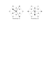
Figure 3: Two different possibilities for neighbourhood of vertex $v$ with $deg_{G_{2}}(v)=4$ in a triangle-free cannonball graph, obtained from the layer-arrangement (a). Circles represent vertices of the middle layer, squares of the upper layer and triangles of the lower layer, and white vertices are part of the grid, but are not in the graph.

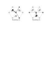
Figure 4: Two different possibilities for vertex $v$ neighbourhood with $deg_{G_{2}}(v)=4$ in a triangle-free cannonball graph, obtained from the layer-arrangement (b). Notation has the same meaning as in Figure 3.

By Lemma 4.3 we know that borrowing is possible for all vertices of degree 4.

In Step 3 we take the colors from the free base color palettes. Without loss of generality, assume that $bc(v)=0$ and one of its free color is 1. Recall the function $D_{1}$ from page 4 – we have $D_{1}(v)$ free colors from the first base color palette. We claim that

Lemma 4.4

$$d_{2}(v)\leq D_{1}(v)$$

Proof:  Let $v$ be a vertex in $G_{2}$ with $bc(v)=0$. If vertex $v\in G_{2}$ has four neighbors in $G_{2}$, it always has such free colors that all neighbors on its layer of this base colors are not in $V(G_{2})$ (see Figures 3 and 4). Without loss of generality assume that one of these free colors is 1. Let $t$ be a vertex, which is an existing neighbor of $v$ in $G_{2}$, and $u$ is the neighbor of $v$ with $bc(u)=1$ so that $\{u,v,t\}\in\tau(T)$ is a triangle. Then we have

$$\kappa(v)+d_{2}(v)+a(u,v,t)+d(u)\stackrel{{\scriptstyle\star}}{{\leq}}d(v)+d(t)+d(u)\leq 3a(u,v,t)\leq a(u,v,t)+2\kappa(v)$$

and the inequality $\star$ occurs because $d_{2}(v)=d(v)-\kappa(v)$ and $d(t)>\kappa(t)\geq a(u,v,t)$. Since vertex $u$ has to belong to the triangle $\{u,v,t\}\in\tau(T)$ where $t$ is a heavy vertex in $G$, it holds $d_{2}(v)\leq\kappa(v)-d(u)$ and finally $d_{2}(v)\leq D_{1}(v).$

In Step 4 we have to prove that for $G_{3}$ we can apply Procedure 2.2. We know that $\Delta(G_{3})\leq 3$ since $\Delta(G_{2})\leq 4$ and in Step 3 we had fully colored all vertices with degree equal to 4. According to theorem of Brooks [3] we know that $G_{3}$ is 3-colorable. Therefore, we can apply Procedure 2.2 and multicolor $G_{3}$ by using $\frac{3}{2}\omega(G_{3})$ new colors.

Ratio

We claim that during the first three steps our algorithm uses at most $\frac{4}{3}\omega_{3}(G)+O(1)$ colors. To see this, notice that in Step 1 each vertex $v$ uses at most $\kappa(v)$ colors from its base color palette and, by Fact 2.1 and using that there are four base colors, we know that no more than $4\left\lceil\omega(G)/3\right\rceil\leq\frac{4}{3}\omega(G)+O(1)$ colors are needed. Note also that in Step 2 and Step 3 we use only those colors from the base color palettes which were not used in Step 1, so altogether no more than $\frac{4}{3}\omega(G)+O(1)$ colors from the base color palettes are used in total until Step 4.

In Step 4 we introduce new palettes that contain no more than $\left\lceil\frac{3}{2}\omega(G_{3})\right\rceil$ colors (by Lemma 2.1) .

Let $A(G)$ denote the number of colors used by our algorithm for the graph $G$. Thus, since $\omega(G_{3})\leq\lceil\omega(G)/3\rceil\leq\omega(G)/3+O(1)$, the total number of colors used by our algorithm is at most

$$A(G)\leq\frac{4}{3}\omega(G)+\frac{3}{2}\omega(G_{3})+O(1)=\frac{4}{3}\omega(G)+\frac{3}{6}\omega(G)+O(1)=\frac{11}{6}\omega(G)+O(1).$$

The performance ratio for our algorithm is $11/6$, hence we arrived at the statement of Theorem 1.1.

5 Conclusion

In this paper we provide an algorithm for a proper multicoloring of a cannonball graph that uses at most $\frac{11}{6}\omega(G)+C$ colors. As this is the first result for the multicoloring problem of cannonball graphs, we belive that further improvements can be done. Among the interesting problems that remain open are improvement of the competitive ratio $11/6$, finding some distributed algorithms for multicoloring cannonball graphs, or finding some $k$-local algorithms for some $k$, similarly as in 2D case for hexagonal graphs (for definition of $k$-local algorithms see [9]). We already mentioned that in the 2D case, better bounds were obtained for triangle-free hexagonal graphs. It is very likely that also for cannonball graphs there exist some ”forbidden” subgraphs $H$, maybe tetrahedrons, such that better bounds can be obtained for $H$-free cannonball graphs.

References

- [1] K. Aardal, S van Hoesel, A koster, C. Mannino, A.Sassano, Models and solution techniques for frequency assignment problems, Ann Oper Res 153 (2007) 79-129.
- [2] L. G. Anderson, A simulation study of some dynamic channel assignment algorithms in a high capacity mobile telecommunication system, IEEE Transaction on Communications 21 (1973) 1294-1301.
- [3] R. L. Brooks, On coloring the nodes of a network, Proceedings of the Cambridge Philosophical Society, vol 37(2), (1941) 118-121.
- [4] W.K. Hale, Frequency assignment: theory and applications, Proceedings of the IEEE, vol 68(12), pp 1497-1514 (1980)
- [5] T. Hales, Cannonballs and honeycombs, Notices of the American Mathematical Society 47 (2000) 440-449.
- [6] T. Hales, A proof of the Kepler conjecture, Annals of Mathematics. Second Series 162 (2005) 1065-1185.
- [7] F. Havet, Channel assignment and multicoloring of the induced subgraphs of the triangular lattice, Discrete Mathematics, vol. 233, pp 219-231 (2001)
- [8] F. Havet, J. Žerovnik, Finding a Five Bicolouring of a Triangle-free Subgraph of the Triangular Lattice, Discrete Mathematics vol. 244, pp 103-108 (2002)
- [9] J. Janssen, D. Krizanc, L. Narayanan, S. Shende, Distributed Online Frequency Assignment in Cellular Network, Journal of Algorithms, vol. 36(2), pp 119-151 (2000)
- [10] C. McDiarmid, B. Reed, Channel assignment and weighted coloring, Networks, vol. 36(2), pp. 114-117 (2000)
- [11] L. Narayanan, Channel assignment and graph multicoloring, Handbook of wireless networks and mobile computing, pp 71-94, Wiley, New York, (2002)
- [12] L. Narayanan, S.M. Shende, Static frequency assignment in cellular networks, Algorithmica, vol. 29(3), pp 396-409 (2001)
- [13] I. Sau, P. Šparl, J. Žerovnik, 7/6-approximation Algorithm for Multicoloring Triangle-free Hexagonal Graphs, Discrete Mathematics, vol. 312, pp 181-187 (2012)
- [14] P. Šparl, R. Witkowski, J. Žerovnik, A Linear Time Algorithm for -coloring Triangle-free Hexagonal Graphs, Information Processing Letters, vol. 112, pp. 567-571 (2012)
- [15] P. Šparl, R. Witkowski, J. Žerovnik, 1-local 7/5-Competitive Algorithm for Multicoloring Hexagonal Graphs, Algorithmica, vol. 64, pp. 564-583 (2012)
- [16] P. Šparl, J. Žerovnik, 2-local 4/3-competitive Algorithm for Multicoloring Hexagonal Graphs, Journal of Algorithms, vol. 55(1), pp 29-41 (2005)
- [17] P. Šparl, J. Žerovnik, 2-local 5/4-competitive algorithm for multicoloring triangle-free hexagonal graphs, Information Processing Letters, vol. 90(5), pp 239-246 (2004)
- [18] P. Šparl, J. Žerovnik, 2-local 7/6-competitive algorithm for multicoloring a sub-class of hexagonal graph, International Journal of Computer Mathematics, vol. 87, pp 2003-2013 (2010)
- [19] K.S. Sudeep, S. Vishwanathan, A technique for multicoloring triangle-free hexagonal graphs, Discrete Mathematics, vol. 300, pp. 256-259 (2005)
- [20] B.H. Yandell, The Honors Class. Hilbert’s Problems and Their Solvers, A K Peters, 2002.
- [21] R. Witkowski, A 1-local 17/12-competitive Algorithm for Multicoloring Hexagonal Graphs, Lecture Notes of Computer Science, vol. 5699/2009, pp 346-356 (2009)
- [22] R. Witkowski, 1-local 4/3-competitive Algorithm for Multicoloring a Subclass of Hexagonal Graphs, in press in Discrete Applied Mathematics (2012), DOI: 10.1016/j.dam.2011.12.013
- [23] R. Witkowski, J. Žerovnik, 1-local 7/5-competitive Algorithm for Multicoloring Hexagonal Graphs, Electronic Notes in Discrete Mathematics, vol 36, pp 375-382 (2010)
- [24] R. Witkowski, J. Žerovnik, 1-local 33/24-competitive Algorithm for Multicoloring Hexagonal Graphs, Lecture Notes of Computer Science, vol 6732, pp 74-84 (2011)
- [25] J. Žerovnik, A distributed 6/5-competitive algorithm for multicoloring triangle-free hexagonal graphs, International Journal of Pure and Applied Mathematics, vol. 23(2), pp 141-156 (2005)
- [26] Algorithmische Graphentheorie, Oberwolfach, December 8-14, 2002. (Report No. 55/2002). Oberwolfach: Mathematisches Forschungsinstitut, 2002. (seminar page http://www.mfo.de/occasion/0250/www_view, link to report www.mfo.de/document/0250/Report55_2002.ps)
- [27] FAP website, http://fap.zib.de/