Observations and three-dimensional ionization structure
of the planetary nebula SuWt 2

Abstract

The planetary nebula SuWt 2 (PN G311.0+02.4), is an unusual object with a prominent, inclined central emission ellipse and faint bipolar extensions. It has two A-type stars in a proven binary system at the centre. However, the radiation from these two central stars is too soft to ionize the surrounding material leading to a so far fruitless search for the responsible ionizing source. Such a source is clearly required and has already been inferred to exist via an observed temporal variation of the centre-of-mass velocity of the A-type stars. Moreover, the ejected nebula is nitrogen-rich which raises question about the mass-loss process from a likely intermediate-mass progenitor. We use optical integral-field spectroscopy to study the emission lines of the inner nebula ring. This has enabled us to perform an empirical analysis of the optical collisionally excited lines, together with a fully three-dimensional photoionization modelling. Our empirical results are used to constrain the photoionization models, which determine the evolutionary stage of the responsible ionizing source and its likely progenitor. The time-scale for the evolutionary track of a hydrogen-rich model atmosphere is inconsistent with the dynamical age obtained for the ring. This suggests that the central star has undergone a very late thermal pulse. We conclude that the ionizing star could be hydrogen-deficient and compatible with what is known as a PG 1159-type star. The evolutionary tracks for the very late thermal pulse models imply a central star mass of $\sim 0.64{\rm M}_{\bigodot}$, which originated from a $\sim 3{\rm M}_{\bigodot}$ progenitor. The evolutionary time-scales suggest that the central star left the asymptotic giant branch about 25,000 years ago, which is consistent with the nebula’s age.

1 Introduction

The southern planetary nebula (PN) SuWt 2 (PN G311.0+02.4) is a particularly exotic object. It appears as an elliptical ring-like nebula with much fainter bipolar lobes extending perpendicularly to the ring, and with what appears to be an obvious, bright central star. The inside of the ring is apparently empty, but brighter than the nebula’s immediate surroundings. An overall view of this ring-shaped structure and its surrounding environment can be seen in the H$\alpha$ image available from the SuperCOSMOS H$\alpha$ Sky Survey (SHS; Parker et al., 2005). West (1976) classified SuWt 2 as of intermediate excitation class (EC; $p=6$–$7$; Aller & Liller, 1968) based on the strength of the He ii $\lambda$4686 and [O ii] $\lambda$3728 doublet lines. The line ratio of [N ii] $\lambda$6584 and H$\alpha$ illustrated by Smith et al. (2007) showed a nitrogen-rich nebula that most likely originated from post-main-sequence mass-loss of an intermediate-mass progenitor star.

Over a decade ago, Bond (2000) discovered that the apparent central star of SuWt 2 (NSV 19992) is a detached double-lined eclipsing binary consisting of two early A-type stars of nearly identical type. Furthermore, Bond et al. (2002) suggested that this is potentially a triple system consisting of the two A-type stars and a hot, unseen PN central star. However, to date, optical and UV studies have failed to find any signature of the nebula’s true ionizing source (e.g. Bond et al., 2002, 2003; Exter et al., 2003, 2010). Hence the putative hot (pre-)white dwarf would have to be in a wider orbit around the close eclipsing pair. Exter et al. (2010) recently derived a period of 4.91 d from time series photometry and spectroscopy of the eclipsing pair, and concluded that the centre-of-mass velocity of the central binary varies with time, based on different systemic velocities measured over the period from 1995 to 2001. This suggests the presence of an unseen third orbiting body, which they concluded is a white dwarf of $\sim 0.7{\rm M}_{\bigodot}$, and is the source of ionizing radiation for the PN shell.

There is also a very bright B1Ib star, SAO 241302 (HD 121228), located 73 arcsec northeast of the nebula. Smith et al. (2007) speculated that this star is the ionizing source for SuWt 2. However, the relative strength of He ii $\lambda$4686 in our spectra (see later) shows that the ionizing star must be very hot, $T$ $>$ 100,000 K, so the B1 star is definitively ruled out as the ionizing source.

Narrow-band H$\alpha$+[N ii] and [O iii] 5007 images of SuWt 2 obtained by Schwarz et al. (1992) show that the angular dimensions of the bright elliptical ring are about $86.5$ arcsec $\times$ $43.4$ arcsec at the 10% of maximum surface brightness isophote (Tylenda et al., 2003), and are used throughout this paper. Smith et al. (2007) used the MOSAIC2 camera on the Cerro Tololo Inter-American Observatory (CTIO) 4-m telescope to obtain a more detailed H$\alpha$+[N ii] image, which hints that the ring is possibly the inner edge of a swept-up disc. The [N ii] image also shows the bright ring structure and much fainter bipolar lobes extending perpendicular to the ring plane. We can see similar structure in the images taken by Bond and Exter in 1995 with the CTIO 1.5 m telescope using an H$\alpha$+[N ii] filter. Fig. 1 shows both narrow-band [N ii] 6584 Å and H$\alpha$ images taken in 1995 with the ESO 3.6 m New Technology Telescope at the La Silla Paranal Observatory using the ESO Multi-Mode Instrument (EMMI). The long-slit emission-line spectra also obtained with the EMMI (programme ID 074.D-0373) in 2005 revealed much more detail of the nebular morphology. The first spatio-kinematical model using the EMMI long-slit data by Jones et al. (2010) suggested the existence of a bright torus with a systemic heliocentric radial velocity of $-25\pm 5$ km s^-1 encircling the waist of an extended bipolar nebular shell.

In this paper, we aim to uncover the properties of the hidden hot ionizing source in SuWt 2. We aim to do this by applying a self-consistent three-dimensional photoionization model using the mocassin 3d code by Ercolano et al. (2003a, 2005, 2008). In Section 2, we describe our optical integral field observations as well as the data reduction process and the corrections for interstellar extinction. In Section 3, we describe the kinematics. In Section 4, we present our derived electron temperature and density, together with our empirical ionic abundances in Section 5. In Section 6, we present derived ionizing source properties and distance from our self-consistent photoionization models, followed by a conclusion in Section 7.

2 Observations and data reduction

Integral-field spectra of SuWt 2 were obtained during two observing runs in 2009 May and 2012 August with the Wide Field Spectrograph (WiFeS; Dopita et al., 2007). WiFeS is an image-slicing Integral Field Unit (IFU) developed and built for the ANU 2.3-m telescope at the Siding Spring Observatory, feeding a double-beam spectrograph. WiFeS samples 0.5 arcsec along each of twenty five $38$ arcsec  $\times$  $1$ arcsec slits, which provides a field-of-view of $25$ arcsec $\times$ $38$ arcsec and a spatial resolution element of $1.0$ arcsec $\times$ $0.5$ arcsec (or $1\hbox{${}^{\prime\prime}$}\times 1\hbox{${}^{\prime\prime}$}$ for y-binning=2). The spectrograph uses volume phase holographic gratings to provide a spectral resolution of $R=3000$ (100 km s^-1 full width at half-maximum, FWHM), and $R=7000$ (45 km s^-1 FWHM) for the red and blue arms, respectively. Each grating has a different wavelength coverage. It can operate two data accumulation modes: classical and nod-and-shuffle (N&S). The N&S accumulates both object and nearby sky-background data in either equal exposures or unequal exposures. The complete performance of the WiFeS has been fully described by Dopita et al. (2007, 2010).

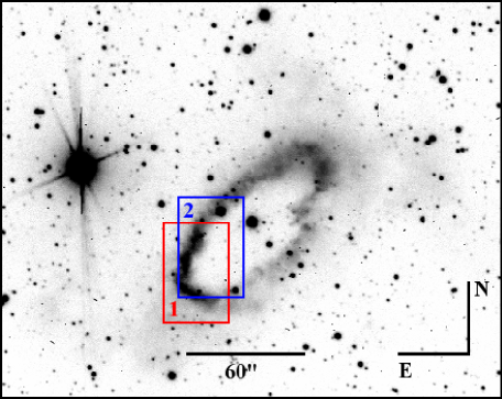
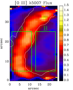
Figure 1: Top panel: narrow-band filter image of the PN SuWt 2 on a logarithmic scale in H$\alpha$ and [N ii] 6584 Å taken with the European Southern Observatory (ESO) 3.6-m telescope (programme ID 055.D-0550). The rectangles correspond to the WiFeS fields of view used for our study: 1 (red) and 2 (blue); see Table LABEL:suwt2:tab:observations for more details. Bottom panels: Spatial distribution maps of flux intensity and continuum of $[$O iii$]$ $\lambda$5007 for field 2 and locations of apertures ($10$ arcsec $\times$ $20$ arcsec) used to integrate fluxes, namely ‘A’ the ring and ‘B’ the interior structure. The white contour lines show the distribution of the above narrow-band H$\alpha$ emission in arbitrary unit. North is up and east is towards the left-hand side.

Our observations were carried out with the B3000/R3000 grating combination and the RT 560 dichroic using N&S mode in 2012 August; and the B7000/R7000 grating combination and the RT 560 dichroic using the classical mode in 2009 May. This covers $\lambda\lambda$3300–5900 Å in the blue channel and $\lambda\lambda$5500–9300 Å in the red channel. As summarized in Table LABEL:suwt2:tab:observations, we took two different WiFeS exposures from different positions of SuWt 2; see Fig. 1 (top). The sky field was collected about 1 arcmin away from the object. To reduce and calibrate the data, it is necessary to take the usual bias frames, dome flat-field frames, twilight sky flats, ‘wire’ frames and arc calibration lamp frames. Although wire, arc, bias and dome flat-field frames were collected during the afternoon prior to observing, arc and bias frames were also taken through the night. Twilight sky flats were taken in the evening. For flux calibration, we also observed some spectrophotometric standard stars.

Table 1: Journal of SuWt 2 Observations at the ANU 2.3-m Telescope.

Field	1	2
Instrument	WiFeS	WiFeS
Wavelength Resolution	$\sim 7000$	$\sim 3000$
Wavelength Range (Å)	4415–5589,	3292–5906,
	5222–7070	5468–9329
Mode	Classical	N&S
Y-Binning	1	2
Object Exposure (s)	$900$	$1200$
Sky Exposure (s)	–	$600$
Standard Star	LTT 3218	LTT 9491,
		HD 26169
$v_{\rm LSR}$ correction	$-5.51$	$-25.77$
Airmass	$1.16$	$1.45$
Position (see Fig. 1)	13:55:46.2	13:55:45.5
	$-59$:22:57.9	$-59$:22:50.3
Date (UTC)	16/05/09	20/08/12

2.1 WiFeS data reduction

The WiFeS data were reduced using the wifes pipeline (updated on 2011 November 21), which is based on the Gemini iraf package (version 1.10; iraf version 2.14.1) developed by the Gemini Observatory for the integral-field spectroscopy.

Each CCD pixel in the WiFeS camera has a slightly different sensitivity, giving pixel-to-pixel variations in the spectral direction. This effect is corrected using the dome flat-field frames taken with a quartz iodine (QI) lamp. Each slitlet is corrected for slit transmission variations using the twilight sky frame taken at the beginning of the night. The wavelength calibration was performed using Ne–Ar arc exposures taken at the beginning of the night and throughout the night. For each slitlet the corresponding arc spectrum is extracted, and then wavelength solutions for each slitlet are obtained from the extracted arc lamp spectra using low-order polynomials. The spatial calibration was accomplished by using so called ‘wire’ frames obtained by diffuse illumination of the coronagraphic aperture with a QI lamp. This procedure locates only the centre of each slitlet, since small spatial distortions by the spectrograph are corrected by the WiFeS cameras. Each wavelength slice was also corrected for the differential atmospheric refraction by relocating each slice in $x$ and $y$ to its correct spatial position.

In the N&S mode, the sky spectra are accumulated in the unused 80 pixel spaces between the adjacent object slices. The sky subtraction is conducted by subtracting the image shifted by 80 pixels from the original image. The cosmic rays and bad pixels were removed from the raw data set prior to sky subtraction using the iraf task LACOS_IM of the cosmic ray identification procedure of van Dokkum (2001), which is based on a Laplacian edge detection algorithm. However, a few bad pixels and cosmic rays still remained in raw data, and these were manually removed by the iraf/stsdas task IMEDIT.

We calibrated the science data to absolute flux units using observations of spectrophotometric standard stars observed in classical mode (no N&S), so sky regions within the object data cube were used for sky subtraction. An integrated flux standard spectrum is created by summing all spectra in a given aperture. After manually removing absorption features, an absolute calibration curve is fitted to the integrated spectrum using third-order polynomials. The flux calibration curve was then applied to the object data to convert to an absolute flux scale. The $[$O i$]\,\lambda$5577Å night sky line was compared in the sky spectra of the red and blue arms to determine a difference in the flux levels, which was used to scale the blue spectrum of the science data. Our analysis using different spectrophotometric standard stars (LTT 9491 and HD 26169) revealed that the spectra at the extreme blue have an uncertainty of about 30% and are particularly unreliable for faint objects due to the CCD’s poor sensitivity in this area.

2.2 Nebular spectrum and reddening

Table LABEL:suwt2:tab:obslines represents a full list of observed lines and their measured fluxes from different apertures ($10$ arcsec $\times$ $20$ arcsec) taken from field 2: (A) the ring and (B) the inside of the shell. Fig. 1 (bottom panel) shows the location and area of each aperture in the nebula. The top and bottom panels of Fig. 2 show the extracted blue and red spectra after integration over the aperture located on the ring with the strongest lines truncated so the weaker features can be seen. The emission line identification, laboratory wavelength, multiplet number, the transition with the lower- and upper-spectral terms, are given in columns 1–4 of Table LABEL:suwt2:tab:obslines, respectively. The observed fluxes of the interior and ring, and the fluxes after correction for interstellar extinction are given in columns 5–8. Columns 9 and 10 present the integrated and dereddened fluxes after integration over two apertures (A and B). All fluxes are given relative to H$\beta$, on a scale where ${\rm H}\beta=100$.

Table 2: Observed and dereddened relative line fluxes, on a scale where ${\rm H}\beta=100$. The integrated observed H($\beta$) flux was dereddened using $c({\rm H}\beta)$ to give an integrated dereddened flux. Uncertain (errors of 20%) and very uncertain (errors of 30%) values are followed by “:” and “::”, respectively. The symbol ‘*’ denotes doublet emission lines.

Region				Interior		Ring		Total
Line	$\lambda_{\rm lab}$(Å)	Mult	Transition	$F(\lambda)$	$I(\lambda)$	$F(\lambda)$	$I(\lambda)$	$F(\lambda)$	$I(\lambda)$
(1)	(2)	(3)	(4)	(5)	(6)	(7)	(8)	(9)	(10)
3726 $[$O ii$]$	3726.03	F1	$2{\rm p}^{3}\,{}^{4}{\rm S}_{3/2}-2{\rm p}^{3}\,{}^{2}{\rm D}_{3/2}$	$183\pm 54$	$307\pm 91$	$576\pm 172$	$815\pm 244$	$479\pm 143$	$702\pm 209$
3729 $[$O ii$]$	3728.82	F1	$2{\rm p}^{3}\,{}^{4}{\rm S}_{3/2}-2{\rm p}^{3}\,{}^{2}{\rm D}_{5/2}$	*	*	*	*	*	*
3869 $[$Ne iii$]$	3868.75	F1	$2{\rm p}^{4}\,{}^{3}{\rm P}_{2}-2{\rm p}^{4}\,{}^{1}{\rm D}_{2}$	128.93::	199.42::	144.31::	195.22::	145.82::	204.57::
3967 $[$Ne iii$]$	3967.46	F1	$2{\rm p}^{4}\,{}^{3}{\rm P}_{1}-2{\rm p}^{4}\,{}^{1}{\rm D}_{2}$	–	–	15.37::	20.26::	–	–
4102 H$\delta$	4101.74	H6	$2{\rm p}\,{}^{2}{\rm P}-6{\rm d}\,{}^{2}{\rm D}$	–	–	16.19:	20.55:	16.97:	22.15:
4340 H$\gamma$	4340.47	H5	$2{\rm p}\,{}^{2}{\rm P}-5{\rm d}\,{}^{2}{\rm D}$	24.47::	31.10::	30.52:	36.04:	31.69:	38.18:
4363 $[$O iii$]$	4363.21	F2	$2{\rm p}^{2}\,{}^{1}{\rm D}_{2}-2{\rm p}^{2}\,{}^{1}{\rm S}_{0}$	37.02::	46.58::	5.60	6.57	5.15	6.15
4686 He ii	4685.68	3-4	$3{\rm d}\,{}^{2}{\rm D}-4{\rm f}\,{}^{2}{\rm F}$	80.97	87.87	29.98	31.72	41.07	43.76
4861 H$\beta$	4861.33	H4	$2{\rm p}\,{}^{2}{\rm P}-4{\rm d}\,{}^{2}{\rm D}$	100.00	100.00	100.00	100.00	100.00	100.00
4959 $[$O iii$]$	4958.91	F1	$2{\rm p}^{2}\,{}^{3}{\rm P}_{1}-2{\rm p}^{2}\,{}^{1}{\rm D}_{2}$	390.90	373.57	173.63	168.27	224.48	216.72
5007 $[$O iii$]$	5006.84	F1	$2{\rm p}^{2}\,{}^{3}{\rm P}_{2}-2{\rm p}^{2}\,{}^{1}{\rm D}_{2}$	1347.80	1259.76	587.22	560.37	763.00	724.02
5412 He ii	5411.52	4-7	$4{\rm f}\,{}^{2}{\rm F}-7{\rm g}\,{}^{2}{\rm G}$	19.33	15.01	5.12	4.30	6.90	5.68
5755 $[$N ii$]$	5754.60	F3	$2{\rm p}^{2}\,{}^{1}{\rm D}_{2}-2{\rm p}^{2}\,{}^{1}{\rm S}_{0}$	7.08:	4.90:	13.69	10.61	10.17	7.64
5876 He i	5875.66	V11	$2{\rm p}\,{}^{3}{\rm P}-3{\rm d}\,{}^{3}{\rm D}$	–	–	11.51	8.69	8.96	6.54
6548 $[$N ii$]$	6548.10	F1	$2{\rm p}^{2}\,{}^{3}{\rm P}_{1}-2{\rm p}^{2}\,{}^{1}{\rm D}_{2}$	115.24	63.13	629.36	414.79	513.64	321.94
6563 H$\alpha$	6562.77	H3	$2{\rm p}\,{}^{2}{\rm P}-3{\rm d}\,{}^{2}{\rm D}$	524.16	286.00	435.14	286.00	457.70	286.00
6584 $[$N ii$]$	6583.50	F1	$2{\rm p}^{2}\,{}^{3}{\rm P}_{2}-2{\rm p}^{2}\,{}^{1}{\rm D}_{2}$	458.99	249.05	1980.47	1296.67	1642.12	1021.68
6678 He i	6678.16	V46	$2{\rm p}\,{}^{1}{\rm P}_{1}-3{\rm d}\,{}^{1}{\rm D}_{2}$	–	–	3.30	2.12	2.68	1.63
6716 $[$S ii$]$	6716.44	F2	$3{\rm p}^{3}\,{}^{4}{\rm S}_{3/2}-3{\rm p}^{3}\,{}^{2}{\rm D}_{5/2}$	60.63	31.77	131.84	84.25	116.21	70.36
6731 $[$S ii$]$	6730.82	F2	$3{\rm p}^{3}\,{}^{4}{\rm S}_{3/2}-3{\rm p}^{3}\,{}^{2}{\rm D}_{3/2}$	30.08	15.70	90.39	57.61	76.98	46.47
7005 [Ar V]	7005.40	F1	$3{\rm p}^{2}\,{}^{3}{\rm P}-3{\rm p}^{2}\,{}^{1}{\rm D}$	5.46:	2.66:	–	–	–	–
7136 $[$Ar iii$]$	7135.80	F1	$3{\rm p}^{4}\,{}^{3}{\rm P}_{2}-3{\rm p}^{4}\,{}^{1}{\rm D}_{2}$	31.81	15.03	26.22	15.59	27.75	15.51
7320 $[$O ii$]$	7319.40	F2	$2{\rm p}^{3}\,{}^{2}{\rm D}_{5/2}-2{\rm p}^{3}\,{}^{2}{\rm P}$	18.84	8.54	9.00	5.20	10.96	5.93
7330 $[$O ii$]$	7329.90	F2	$2{\rm p}^{3}\,{}^{2}{\rm D}_{3/2}-2{\rm p}^{3}\,{}^{2}{\rm P}$	12.24	5.53	4.50	2.60	6.25	3.37
7751 $[$Ar iii$]$	7751.43	F1	$3{\rm p}^{4}\,{}^{3}{\rm P}_{1}-3{\rm p}^{4}\,{}^{1}{\rm D}_{2}$	46.88	19.38	10.97	5.95	19.05	9.60
9069 $[$S iii$]$	9068.60	F1	$3{\rm p}^{2}\,{}^{3}{\rm P}_{1}-3{\rm p}^{2}\,{}^{1}{\rm D}_{2}$	12.32	4.07	13.27	6.16	13.34	5.65
$c({\rm H}\beta)$				–	0.822	–	0.569	–	0.638

For each spatially resolved emission line profile, we extracted flux intensity, central wavelength (or centroid velocity), and FWHM (or velocity dispersion). Each emission line profile for each spaxel is fitted to a single Gaussian curve using the mpfit routine (Markwardt, 2009), an idl version of the minpack-1 fortran code (Moré, 1977), which applies the Levenberg–Marquardt technique to the non-linear least-squares problem. Flux intensity maps of key emission lines of field 2 are shown in Fig. 3 for $[$O iii$]$ $\lambda$5007, H$\alpha$ $\lambda$6563, $[$N ii$]$ $\lambda$6584 and $[$S ii$]$ $\lambda$6716; the same ring morphology is visible in the $[$N ii$]$ map as seen in Fig. 1. White contour lines in the figures depict the distribution of the narrow-band emission of H$\alpha$ and $[$N ii$]$ taken with the ESO 3.6 m telescope, which can be used to distinguish the borders between the ring structure and the inside region. We excluded the stellar continuum offset from the final flux maps using mpfit, so spaxels show only the flux intensities of the nebulae.

Figure 2: The observed optical spectrum from an aperture $10$ arcsec $\times$ $20$ arcsec taken from field 2 located on the east ring of the PN SuWt 2 and normalized such that $F({\rm H}\beta)=100$.

The H$\alpha$ and H$\beta$ Balmer emission-line fluxes were used to derive the logarithmic extinction at H$\beta$, $c({\rm H}\beta)=\log[I({\rm H}\beta)/F({\rm H}\beta)]$, for the theoretical line ratio of the case B recombination ($T_{\rm e}=10\,000$ K and $N_{\rm e}=100$ cm^-3; Hummer & Storey, 1987). Each flux at the central wavelength was corrected for reddening using the logarithmic extinction $c({\rm H}\beta)$ according to

$$I(\lambda)=F(\lambda)\,10^{c({\rm H}\beta)[1+f(\lambda)]},$$ (1)

where $F(\lambda)$ and $I(\lambda)$ are the observed and intrinsic line flux, respectively, and $f(\lambda)$ is the standard Galactic extinction law for a total-to-selective extinction ratio of $R_{V}\equiv A(V)/E(B-V)=3.1$ (Seaton, 1979b, a; Howarth, 1983).

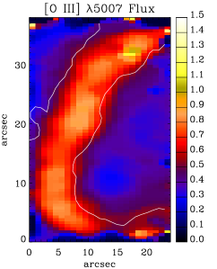
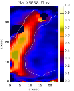
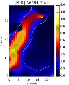
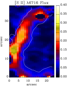
Figure 3: Undereddened flux maps for field 2 (see Fig. 1) of the PN SuWt 2: $[$O iii$]$ $\lambda$5007, H$\alpha$ $\lambda$6563, $[$N ii$]$ $\lambda$6584 and $[$S ii$]$ $\lambda$6716. The flux is derived from single Gaussian profile fits to the emission line at each spaxel. The white contour lines show the distribution of the narrow-band emission of H$\alpha$ and [N ii] in arbitrary unit taken with the ESO 3.6-m telescope. North is up and east is towards the left-hand side. Flux unit is in $10^{-15}$ erg s^-1 cm^-2 spaxel^-1.

Accordingly, we obtained an extinction of $c({\rm H}\beta)=0.64$ [$E(B-V)=0.44$] for the total fluxes (column 9 in Table LABEL:suwt2:tab:obslines). Our derived nebular extinction is in good agreement with the value found by Exter et al. (2010), $E(B-V)=0.40$ for the central star, though they obtained $E(B-V)=0.56$ for the nebula. It may point to the fact that all reddening is not due to the interstellar medium (ISM), and there is some dust contribution in the nebula. Adopting a total observed flux value of log$F$(H$\alpha$) = $-11.69$ erg cm^-2 s^-1 for the ring and interior structure (Frew, 2008; Frew et al., 2013a, b) and using $c({\rm H}\beta)=0.64$, lead to the dereddened H$\alpha$ flux of log$I$(H$\alpha$) = $-11.25$ erg cm^-2 s^-1.

According to the strength of He ii $\lambda$4686 relative to H$\beta$, the PN SuWt 2 is classified as the intermediate excitation class with ${\rm EC}=6.6$ (Dopita & Meatheringham, 1990) or ${\rm EC}=7.8$ (Reid & Parker, 2010). The EC is an indicator of the central star effective temperature (Dopita & Meatheringham, 1991; Reid & Parker, 2010). Using the $T_{\rm eff}$–EC relation of Magellanic Cloud PNe found by Dopita & Meatheringham (1991), we estimate $T_{\rm eff}=143$ kK for ${\rm EC}=6.6$. However, we get $T_{\rm eff}=177$ kK for ${\rm EC}=7.8$ according to the transformation given by Reid & Parker (2010) for Large Magellanic Cloud PNe.

3 Kinematics

Table 3: Kinematic parameters on the SuWt 2’s ring and its central star.

Parameter	Value
$a=r$ (outer radius)	$45\pm 4$ arcsec
$b=r\cos i$	$17\pm 2$ arcsec
thickness	$13\pm 2$ arcsec
PA	$48^{\circ}\pm 2^{\circ}$
GPA	$62^{\circ}16\hbox{${}^{\prime}$}\pm 2^{\circ}$
inclination ($i$)	$68^{\circ}\pm 2^{\circ}$
$v_{\rm sys}$ (LSR)	$-29.5\pm 5$ km s-1
$v_{\rm exp}$	$28\pm 5$ km s-1

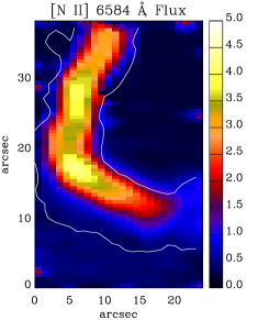
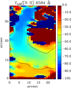
Figure 4: Flux intensity and radial velocity ($V_{\rm LSR}$) map in $[$N ii$]$ $\lambda$ 6584 Å for Field 1 (see Table LABEL:suwt2:tab:observations) of the PN SuWt 2. The white/black contour lines show the distribution of the narrow-band emission of H$\alpha$ and [N ii] in arbitrary unit taken with the ESO 3.6-m telescope. North is up and east is toward the left-hand side. Units are in km s^-1.

Fig. 4 presents maps of the flux intensity and the local standard of rest (LSR) radial velocity derived from the Gaussian profile fits for the emission line $[$N ii$]$ $\lambda$ 6584 Å. We transferred the observed velocity $v_{\rm obs}$ to the LSR radial velocity $v_{\rm lsr}$ by determining the radial velocities induced by the motions of the Earth and Sun using the iraf/astutil task RVCORRECT. The emission-line profile is also resolved if its velocity dispersion is wider than the instrumental width $\sigma_{\rm ins}$. The instrumental width can be derived from the $[$O i$]\,\lambda$5577Å and $\lambda$6300Å night sky lines; it is typically $\sigma_{\rm ins}\approx 42$ km s^-1 for $R\sim 3000$ and $\sigma_{\rm ins}\approx 19$ km s^-1 for $R\sim 7000$. Fig. 4(right) shows the variation of the LSR radial velocity in the south-east side of the nebula. We see that the radial velocity decreases as moving anti-clockwise on the ellipse. It has a low value of about $-70\pm 30$ km s^-1 on the west co-vertex of the ellipse, and a high value of $-50\pm 25$ km s^-1 on the south vertex. This variation corresponds to the orientation of this nebula, namely the inclination and projected nebula on the plane of the sky. It obviously implies that the east side moves towards us, while the west side escapes from us.

Kinematic information of the ring and the central star is summarized in Table LABEL:suwt2:tab:kinematic:parameters. Jones et al. (2010) implemented a morpho-kinematic model using the modelling program shape (Steffen & López, 2006) based on the long-slit emission-line spectra at the high resolution of $R\sim 40\,000$, which is much higher than the moderate resolution of $R\sim 3000$ in our observations. They obtained the nebular expansion velocity of $v_{\rm exp}=28$ km s^-1 and the LSR systemic velocity of $v_{\rm sys}=-29.5\pm 5$ at the best-fitting inclination of $i=68^{\circ}\pm 2^{\circ}$ between the line of sight and the nebular axisymmetry axis. We notice that the nebular axisymmetric axis has a position angle of ${\rm PA}=48^{\circ}$ projected on to the plane of the sky, and measured from the north towards the east in the equatorial coordinate system (ECS). Transferring the PA in the ECS to the PA in the Galactic coordinate system yields the Galactic position angle of ${\rm GPA}=62^{\circ}16\hbox{${}^{\prime}$}$, which is the PA of the nebular axisymmetric axis projected on to the plane of the sky, measured from the North Galactic Pole (NGP; ${\rm GPA}=0^{\circ}$) towards the Galactic east (${\rm GPA}=90^{\circ}$). We notice an angle of $-27^{\circ}44\hbox{${}^{\prime}$}$ between the nebular axisymmetric axis projected onto the plane of the sky and the Galactic plane. Fig. 5 shows the flux ratio map for the $[$S ii$]$ doublet to the H$\alpha$ recombination line emission. The shock criterion $[$S ii$]$ $\lambda\lambda$6716,6731/H$\alpha\geq 0.5$ indicates the presence of a shock-ionization front in the ring. Therefore, the brightest south-east side of the nebula has a signature of an interaction with ISM.

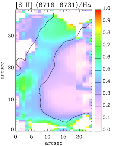
Figure 5: Flux ratio maps of the $[$S ii$]$ $\lambda$ 6716+6731 Å to the H$\alpha$ recombination line emission.

The PPMXL catalogue (Roeser et al., 2010) reveals that the A-type stars of SuWt 2 move with the proper motion of $v_{l}=D\mu_{l}\cos(b)=(-8.09\pm 8.46)D$ km s^-1 and $v_{b}=D\mu_{b}=(11.79\pm 8.82)D$ km s^-1, where $D$ is its distance in kpc. They correspond to the magnitude of $v_{\mu}=(14.30\pm 8.83)D$ km s^-1. Assuming a distance of $D=2.3$ kpc (Exter et al., 2010) and $v_{\rm sys}=-29.5\pm 5$ km s^-1 (LSR; Jones et al., 2010), this PN moves in the Cartesian Galactocentric frame with peculiar (non-circular) velocity components of ($U_{s}$, $V_{s}$, $W_{s})=$ ($35.4\pm 18.4$, $11.0\pm 13.7$, $33.18\pm 26.4$) km s^-1, where $U_{s}$ is towards the Galactic centre, $V_{s}$ in the local direction of Galactic rotation, and $W_{s}$ towards the NGP (see Reid et al., 2009, peculiar motion calculations in appendix). We see that SuWt 2 moves towards the NGP with $W_{s}=33.18$ km s^-1, and there is an interaction with ISM in the direction of its motion, i.e., the east-side of the nebula.

We notice a very small peculiar velocity ($V_{s}=11$ km s^-1) in the local direction of Galactic rotation, so a kinematic distance may also be estimated as the Galactic latitude is a favorable one for such a determination. We used the fortran code for the ‘revised’ kinematic distance prescribed in Reid et al. (2009), and adopted the IAU standard parameters of the Milky Way, namely the distance to the Galactic centre $R_{0}=8.5$ kpc and a circular rotation speed $\Theta_{0}=220$ km s^-1 for a flat rotation curve (${\rm d}\Theta/{\rm d}R=0$), and the solar motion of ${\rm U}_{\bigodot}=10.30$ km s^-1, ${\rm V}_{\bigodot}=15.3$ km s^-1 and ${\rm W}_{\bigodot}=7.7$ km s^-1. The LSR systemic velocity of $-29.5$ km s^-1 (Jones et al., 2010) gives a kinematic distance of $2.26$ kpc, which is in quite good agreement with the distance of 2.3 $\pm$ 0.2 kpc found by Exter et al. (2010) based on an analysis of the double-lined eclipsing binary system. This distance implies that SuWt 2 is in the tangent of the Carina-Sagittarius spiral arm of the Galaxy ($l=311\aas@@fstack{\circ}0$, $b=2\aas@@fstack{\circ}4$). Our adopted distance of 2.3 kpc means the ellipse’s major radius of $45$ arcsec corresponds to a ring radius of $r=0.47\pm 0.04$ pc. The expansion velocity of the ring then yields a dynamical age of $\tau_{\rm dyn}=r/v_{\rm exp}=17500\pm 1560$ yr, which is defined as the radius divided by the constant expansion velocity. Nonetheless, the true age is more than the dynamical age, since the nebula expansion velocity is not constant through the nebula evolution. Dopita et al. (1996) estimated the true age typically around 1.5 of the dynamical age, so we get $\tau_{\rm true}=26250\pm 2330$ yr for SuWt 2. If we take the asymptotic giant branch (AGB) expansion velocity of $v_{\rm AGB}=v_{\rm exp}/2$ (Gesicki & Zijlstra, 2000), as the starting velocity of the new evolving PN, we also estimate the true age as $\tau_{\rm true}=2r/(v_{\rm exp}+v_{\rm AGB})=23360\pm 2080$ yr.

4 Plasma diagnostics

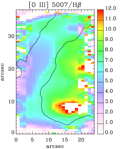
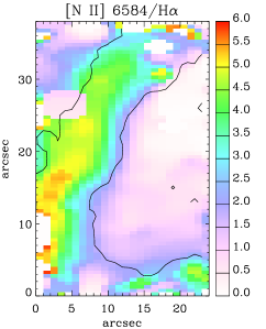
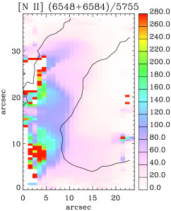
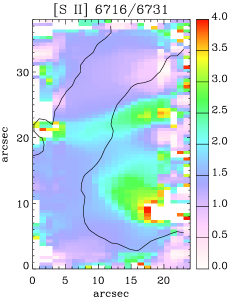
(a)                                   (b)                                   (c)                                   (d)

Figure 6: Flux ratio maps for field 2 (see Fig. 1) of the PN SuWt 2. From left to right: (a) flux ratio maps of the $[$O iii$]$ $\lambda$ 5007 Å to the H$\beta$ recombination line emission, (b) flux ratio map of the $[$N ii$]$ $\lambda$ 6584 to the H$\alpha$ recombination line emission, (c) flux ratio map for the temperature-sensitive $[$N ii$]$ $\lambda\lambda$5755, 6548, 6583 lines, and (d) for the density-sensitive $[$S ii$]$ doublet. The black contour lines show the distribution of the narrow-band emission of H$\alpha$ and [N ii] in arbitrary units taken with the ESO 3.6-m telescope observations.

We derived the nebular electron temperatures $T_{\rm e}$ and densities $N_{\rm e}$ from the intensities of the collisionally excited lines (CELs) by solving the equilibrium equations for an $n$-level atom ($\geqslant 5$) using equib, a fortran code originally developed by Howarth & Adams (1981). Recently, it has been converted to fortran 90, and combined into simpler routines for neat (Wesson et al., 2012). The atomic data sets used for our plasma diagnostics, as well as for the CEL abundance determination in § 5, are the same as those used by Wesson et al. (2012).

The diagnostics procedure was as follows: we assumed a representative initial electron temperature of 10 000 K in order to derive $N_{\rm e}([$S ii$])$; then $T_{\rm e}([$N ii$])$ was derived in conjunction with the mean density derived from $N_{\rm e}([$S ii$])$. The calculations were iterated to give self-consistent results for $N_{\rm e}$ and $T_{\rm e}$. The correct choice of electron density and temperature is essential to determine ionic abundances.

Fig. 6 shows flux ratio maps for the density-sensitive $[$S ii$]$ doublet. It indicates the electron density $N_{\rm e}$ of about $\lesssim 100$ cm^-3 in the ring. We see that the interior region has a $[$S ii$]$ $\lambda\lambda$ 6716/6731 flux ratio of more than 1.4, which means the inside of the ring has a very low density ($N_{\rm e}\lesssim 50$ cm^-3). Flux ratio maps for the temperature-sensitive $[$N ii$]$ $\lambda\lambda$5755, 6548, 6583 lines indicate that the electron temperature $T_{\rm e}$ varies from 7 000 to 14 000 K. As shown in Fig. 6, the brightest part of the ring in $[$N ii$]$ $\lambda$ 6584 Å has an electron temperature of about 8 000 K. The inside of the ring has a mean electron temperature of about 11 800 K. We notice that Smith et al. (2007) found $N_{\rm e}=90$ cm^-3 and $T_{\rm e}=11\,400$ K using the R-C Spectrograph ($R\sim 6000$) on the CTIO 4-m telescope, though they obtained them from a $0.8$ arcsec slit oriented along the major axis of the ring (${\rm PA}=135^{\circ}$).

Table LABEL:suwt2:tab:tenediagnostics lists the electron density ($N_{\rm e}$) and the electron temperature ($T_{\rm e}$) of the different regions, together with the ionization potential required to create the emitting ions. We see that the east part of the ring has a mean electron density of $N_{\rm e}([$S ii$])\lesssim 100$ cm^-3 and mean temperatures of $T_{\rm e}([$N ii$])=8\,140$ K and $T_{\rm e}([$O iii$])=12\,390$ K, while the less dense region inside the ring shows a high mean temperature of $T_{\rm e}([$N ii$])=11\,760$ K and $T_{\rm e}([$O iii$])$ less than $20\,000$ K. We point out that the [S ii] $\lambda\lambda$6716/6731 line ratio of more than 1.40 is associated with the low-density limit of $N_{\rm e}<100$ cm^-3, and we cannot accurately determine the electron density less than this limit (see e.g. A 39; Jacoby et al., 2001). Furthermore, we cannot resolve the [O ii] $\lambda\lambda$3726,3729 doublet with our moderate spectral resolution ($R\sim 3000$). Plasma diagnostics indicates that the interior region is much hotter than the ring region. This implies the presence of a hard ionizing source located at the centre. It is worth to mention that $T_{\rm e}([$N ii$])$ is more appropriate for singly ionized species, while $T_{\rm e}([$O iii$])$ is associated with doubly and more ionized species. Kingsburgh & Barlow (1994) found that $T_{\rm e}([$O iii$])/T_{\rm e}([$N ii$])=1.25$ for medium-excitation PNe and $T_{\rm e}([$O iii$])/T_{\rm e}([$N ii$])=1.15+0.0037I(4686)$ for high-excitation PNe. Here, we notice that $T_{\rm e}([$O iii$])/T_{\rm e}([$N ii$])=1.52$ for the ring and $T_{\rm e}([$O iii$])/T_{\rm e}([$N ii$])=1.39$ for the total flux.

Table 4: Diagnostic ratios for the electron temperature, $T_{\rm e}$ and the electron density, $N_{\rm e}$.

Ion	Diagnostic	I.P.(eV)	Interior		Ring		Total
			Ratio	$T_{\rm e}(10^{3}{\rm K})$	Ratio	$T_{\rm e}(10^{3}{\rm K})$	Ratio	$T_{\rm e}(10^{3}{\rm K})$
$[$N ii$]$	$\frac{\lambda 6548+\lambda 6584}{\lambda 5755}$	14.53	63.71:	11.76:	161.33	8.14	175.78	7.92
$[$O iii$]$	$\frac{\lambda 4959+\lambda 5007}{\lambda 4363}$	35.12	35.41::	$\lesssim 20.0$::	110.93	12.39	152.49	11.07
			Ratio	$N_{\rm e}({\rm cm}^{-3})$	Ratio	$N_{\rm e}({\rm cm}^{-3})$	Ratio	$N_{\rm e}({\rm cm}^{-3})$
$[$S ii$]$	$\frac{\lambda 6716}{\lambda 6731}$	10.36	2.02	$\lesssim 50.0$	1.46	$\lesssim 100.0$	1.51	$\lesssim 100.0$

Table 5: Ionic and total abundances deduced from empirical analysis of the observed fluxes across different nebula regions of SuWt 2.

$\lambda$(Å)	Abundance	Interior	Ring	Total
5876	He+/H+	–	0.066	0.049
6678	He+/H+	0.031	0.057	0.043
Mean	He+/H+	0.031	0.064	0.048
4686	He2+/H+	0.080	0.027	0.036
	$icf$(He)	1.0	1.0	1.0
	He/H	0.111	0.091	0.084
6548	N+/H+	7.932($-6$)	1.269($-4$)	1.284($-4$)
6584	N+/H+	1.024($-5$)	1.299($-4$)	1.334($-4$)
Mean	N+/H+	9.086($-6$)	1.284($-4$)	1.309($-4$)
	$icf$(N)	16.240	2.014	3.022
	N/H	1.476($-4$)	2.587($-4$)	3.956($-4$)
3727	O+/H+	1.109($-5$)	1.576($-4$)	1.597($-4$)
4959	O2+/H+	6.201($-5$)	8.881($-5$)	1.615($-4$)
5007	O2+/H+	6.998($-5$)	9.907($-5$)	1.808($-4$)
Mean	O2+/H+	6.599($-5$)	9.394($-5$)	1.711($-4$)
	$icf$(O)	2.336	1.262	1.459
	O/H	1.801($-4$)	3.175($-4$)	4.826($-4$)
3869	Ne2+/H+	2.635($-5$)	9.608($-5$)	1.504($-4$)
3968	Ne2+/H+	–	3.306($-5$)	–
Mean	Ne2+/H+	2.635($-5$)	6.457($-5$)	1.504($-4$)
	$icf$(Ne)	2.728	3.380	2.820
	Ne/H	7.191($-5$)	2.183($-4$)	4.241($-4$)
6716	S+/H+	3.307($-7$)	2.034($-6$)	2.179($-6$)
6731	S+/H+	2.189($-7$)	1.834($-6$)	1.903($-6$)
Mean	S+/H+	2.748($-7$)	1.934($-6$)	2.041($-6$)
6312	S2+/H+	–	3.292($-8$)	–
9069	S2+/H+	3.712($-7$)	1.198($-6$)	1.366($-6$)
Mean	S2+/H+	3.712($-7$)	6.155($-7$)	1.366($-6$)
	$icf$(S)	1.793	1.047	1.126
	S/H	1.158($-6$)	2.668($-6$)	3.836($-6$)
7136	Ar2+/H+	3.718($-7$)	8.756($-7$)	1.111($-6$)
4740	Ar3+/H+	–	–	4.747($-7$)
7005	Ar4+/H+	3.718($-7$)	–	–
	$icf$(Ar)	1.066	1.986	1.494
	Ar/H	5.230($-7$)	1.739($-6$)	2.370($-6$)

5 Ionic and total abundances

We derived ionic abundances for SuWt 2 using the observed CELs and the optical recombination lines (ORLs). We determined abundances for ionic species of N, O, Ne, S and Ar from CELs. In our determination, we adopted the mean $T_{\rm e}$([O iii]) and the upper limit of $N_{\rm e}$([S ii]) obtained from our empirical analysis in Table LABEL:suwt2:tab:tenediagnostics. Solving the equilibrium equations, using equib, yields level populations and line sensitivities for given $T_{\rm e}$ and $N_{\rm e}$. Once the level population are solved, the ionic abundances, Xⁱ⁺/H⁺, can be derived from the observed line intensities of CELs. We determined ionic abundances for He from the measured intensities of ORLs using the effective recombination coefficients from Storey & Hummer (1995) and Smits (1996). We derived the total abundances from deduced ionic abundances using the ionization correction factor ($icf$) formulae given by Kingsburgh & Barlow (1994):

$$\footnotesize\frac{{\rm He}}{{\rm H}}=\left(\frac{{\rm He}^{+}}{{\rm H}^{+}}+\frac{{\rm He}^{2+}}{{\rm H}^{+}}\right)\times{{icf}}({\rm He}),~{}~{}{{icf}}({\rm He})=1,$$ (2)

$$\footnotesize\frac{{\rm O}}{{\rm H}}=\left(\frac{{\rm O}^{+}}{{\rm H}^{+}}+\frac{{\rm O}^{2+}}{{\rm H}^{+}}\right)\times{{icf}}({\rm O}),~{}~{}{{icf}}({\rm O})=\left(1+\frac{{\rm He}^{2+}}{{\rm He}^{+}}\right)^{2/3},$$ (3)

$$\footnotesize\frac{{\rm N}}{{\rm H}}=\left(\frac{{\rm N}^{+}}{{\rm H}^{+}}\right)\times{{icf}}({\rm N}),~{}~{}{{icf}}({\rm N})=\left(\frac{{\rm O}}{{\rm O}^{+}}\right),$$ (4)

$$\footnotesize\frac{{\rm Ne}}{{\rm H}}=\left(\frac{{\rm Ne}^{2+}}{{\rm H}^{+}}\right)\times{{icf}}({\rm Ne}),~{}~{}{{icf}}({\rm Ne})=\left(\frac{{\rm O}}{{\rm O}^{2+}}\right),$$ (5)

$$\footnotesize\frac{{\rm S}}{{\rm H}}=\left(\frac{{\rm S}^{+}}{{\rm H}^{+}}+\frac{{\rm S}^{2+}}{{\rm H}^{+}}\right)\times{{icf}}({\rm S}),$$ (6)

$$\footnotesize{{icf}}({\rm S})=\left[1-\left(1-\frac{{\rm O}^{+}}{{\rm O}}\right)^{3}\right]^{-1/3},$$ (7)

$$\footnotesize\frac{{\rm Ar}}{{\rm H}}=\left(\frac{{\rm Ar}^{2+}}{{\rm H}^{+}}\right)\times{{icf}}({\rm Ar}),~{}~{}{{icf}}({\rm Ar})=\left(1-\frac{{\rm N}^{+}}{{\rm N}}\right)^{-1}.$$ (8)

We derived the ionic and total helium abundances from the observed $\lambda$5876 and $\lambda$6678, and He ii $\lambda$4686 ORLs. We assumed case B recombination for the singlet He i $\lambda$6678 line and case A for other He i $\lambda$5876 line (theoretical recombination models of Smits, 1996). The He⁺/H⁺ ionic abundances from the He i lines at $\lambda$5876 and $\lambda$6678 were averaged with weights of 3:1, roughly the intrinsic intensity ratios of the two lines. The He²⁺/H⁺ ionic abundances were derived from the He ii $\lambda$4686 line using theoretical case B recombination rates from Storey & Hummer (1995). For high- and middle-EC PNe (E.C. $>4$), the total He/H abundance ratio can be obtained by simply taking the sum of singly and doubly ionized helium abundances, and with an $icf$(He) equal or less than 1.0. For PNe with low levels of ionization it is more than 1.0. SuWt 2 is an intermediate-EC PN (${\rm EC}=6.6$; Dopita & Meatheringham, 1990), so we can use an $icf$(He) of 1.0. We determined the O⁺/H⁺ abundance ratio from the $[$O ii$]$ $\lambda$3727 doublet, and the O²⁺/H⁺ abundance ratio from the $[$O iii$]$ $\lambda$4959 and $\lambda$5007 lines. In optical spectra, only O⁺ and O²⁺ CELs are seen, so the singly and doubly ionized helium abundances deduced from ORLs are used to include the higher ionization stages of oxygen abundance.

Table 6: Parameters of the two best-fitting photoionization models. The initial mass, final mass, and Post-AGB age are obtained from the evolutionary tracks calculated for hydrogen- and helium-burning models by Blöcker (1995)

	Nebula abundances		Stellar parameters
Model 1	He/H	0.090	$T_{\rm eff}$(kK)	140
	C/H	4.00($-4$)	$L_{\star}\,({\rm L}_{\bigodot})$	700
	N/H	2.44($-4$)	$\log\,g$ (cgs)	$7.0$
	O/H	2.60($-4$)	H : He	8 : 2
	Ne/H	1.11($-4$)	$M_{\star}\,({\rm M}_{\bigodot})$	$\sim 0.605$
	S/H	1.57($-6$)	$M_{\rm\textsc{zams}}\,({\rm M}_{\bigodot})$	3.0
	Ar/H	1.35($-6$)	$\tau_{\rm post-\textsc{agb}}$ (yr)	7 500
Model 2	He/H	0.090	$T_{\rm eff}$(kK)	160
	C/H	4.00($-4$)	$L_{\star}\,({\rm L}_{\bigodot})$	600
	N/H	2.31($-4$)	$\log\,g$ (cgs)	$7.3$
	O/H	2.83($-4$)	He : C : N : O	33 : 50 : 2 : 15
	Ne/H	1.11($-4$)	$M_{\star}\,({\rm M}_{\bigodot})$	$\sim 0.64$
	S/H	1.57($-6$)	$M_{\rm\textsc{zams}}\,({\rm M}_{\bigodot})$	3.0
	Ar/H	1.35($-6$)	$\tau_{\rm post-\textsc{agb}}$ (yr)	$25\,000$
	Nebula physical parameters
$M_{i}/{\rm M}_{\bigodot}$		0.21	$D$ (pc)	2 300
$N_{\rm torus}$		100 cm-3	$\tau_{\rm true}$ (yr)	$23\,400$–$26\,300$
$N_{\rm spheroid}$		50 cm-3	$[{\rm Ar/H}]$	$-0.049$

We derived the ionic and total nitrogen abundances from $[$N ii$]$ $\lambda$6548 and $\lambda$6584 CELs. For optical spectra, it is possible to derive only N⁺, which mostly comprises only a small fraction ($\sim 10$-30%) of the total nitrogen abundance. Therefore, the oxygen abundances were used to correct the nitrogen abundances for unseen ionization stages of N²⁺ and N³⁺. Similarly, the total Ne/H abundance was corrected for undetermined Ne³⁺ by using the oxygen abundances. The $\lambda\lambda$6716,6731 lines usually detectable in PN are preferred to be used for the determination of S⁺/H⁺, since the $\lambda\lambda$4069,4076 lines are usually enhanced by recombination contribution, and also blended with O ii lines. We notice that the $\lambda\lambda$6716,6731 doublet is affected by shock excitation of the ISM interaction, so the S⁺/H⁺ ionic abundance must be lower. When the observed S⁺ is not appropriately determined, it is possible to use the expression given by Kingsburgh & Barlow (1994) in the calculation, i.e. $({\rm S}^{2+}/{\rm S}^{+})=4.677+({\rm O}^{2+}/{\rm O}^{+})^{0.433}$.

Table 7: Model line fluxes for SuWt 2.

Line	Observ.	Model 1	Model 2
3726 $[$O ii$]$	$702$::	309.42	335.53
3729 $[$O ii$]$	*	408.89	443.82
3869 $[$Ne iii$]$	204.57::	208.88	199.96
4069 $[$S ii$]$	1.71::	1.15	1.25
4076 $[$S ii$]$	–	0.40	0.43
4102 H$\delta$	22.15:	26.11	26.10
4267 C ii	–	0.27	0.26
4340 H$\gamma$	38.18:	47.12	47.10
4363 $[$O iii$]$	6.15	10.13	9.55
4686 He ii	43.76	42.50	41.38
4740 $[$Ar iv$]$	1.94	2.27	2.10
4861 H$\beta$	100.00	100.00	100.0
4959 $[$O iii$]$	216.72	243.20	238.65
5007 $[$O iii$]$	724.02	725.70	712.13
5412 He ii	5.68	3.22	3.14
5755 $[$N ii$]$	7.64	21.99	21.17
5876 He i	6.54	8.01	8.30
6548 $[$N ii$]$	321.94	335.22	334.67
6563 H$\alpha$	286.00	281.83	282.20
6584 $[$N ii$]$	1021.68	1023.78	1022.09
6678 He i	1.63	2.25	2.33
6716 $[$S ii$]^{\rm\ast}$	70.36	9.17	10.21
6731 $[$S ii$]^{\rm\ast}$	46.47	6.94	7.72
7065 He i	1.12	1.59	1.63
7136 $[$Ar iii$]$	15.51	15.90	15.94
7320 $[$O ii$]$	5.93	10.60	11.17
7330 $[$O ii$]$	3.37	8.64	9.11
7751 $[$Ar iii$]$	9.60	3.81	3.82
9069 $[$S iii$]$	5.65	5.79	5.58
$I($H$\beta)$/10-12 $\frac{\rm erg}{{\rm cm}^{2}{\rm s}}$	1.95	2.13	2.12

Note. ^∗ The shock-excitation largely enhances the observed $[$S ii$]$ doublet.

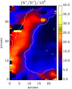
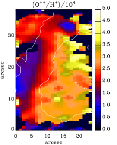
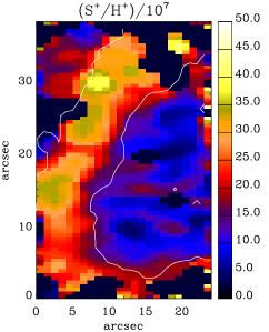
Figure 7: Spatial distribution maps of ionic nitrogen abundance ratio N⁺/H⁺ ($\times 10^{-5}$) from $[$N ii$]$ CELs (6548, 6584); ionic oxygen abundance ratio O⁺⁺/H⁺ ($\times 10^{-4}$) from $[$O iii$]$ CELs (4959, 5007); and ionic Sulfur abundance ratio S⁺/H⁺ ($\times 10^{-7}$) from $[$S ii$]$ CELs (6716, 6731) for $T_{\rm e}=10\,000$ K and $N_{\rm e}=100$ cm^-3. White contour lines show the distribution of the narrow-band emission of H$\alpha$ and [N ii] in arbitrary unit taken with the ESO 3.6-m telescope.

The total abundances of He, N, O, Ne, S, and Ar derived from our empirical analysis for selected regions of the nebula are given in Table LABEL:suwt2:tab:abundances:empirical. From Table LABEL:suwt2:tab:abundances:empirical we see that SuWt 2 is a nitrogen-rich PN, which may be evolved from a massive progenitor ($M\geq 5$). However, the nebula’s age (23 400–26 300 yr) cannot be associated with faster evolutionary time-scale of a massive progenitor, since the evolutionary time-scale of $7{\rm M}_{\bigodot}$ calculated by Blöcker (1995) implies a short time-scale (less than 8000 yr) for the effective temperatures and the stellar luminosity (see Table LABEL:suwt2:tab:obslines) that are required to ionize the surrounding nebula. So, another mixing mechanism occurred during AGB nucleosynthesis, which further increased the Nitrogen abundances in SuWt 2. Mass transfer to the two A-type companions may explain this typical abundance pattern.

Fig. 7 shows the spatial distribution of ionic abundance ratio N⁺/H⁺, O⁺⁺/H⁺ and S⁺/H⁺ derived for given $T_{\rm e}=10\,000$ K and $N_{\rm e}=100$ cm^-3. We notice that O⁺⁺/H⁺ ionic abundance is very high in the inside shell; through the assumption of homogeneous electron temperature and density is not correct. The values in Table LABEL:suwt2:tab:abundances:empirical are obtained using the mean $T_{\rm e}$([O iii]) and $N_{\rm e}$([S ii]) listed in Table LABEL:suwt2:tab:tenediagnostics. We notice that O²⁺/O${}^{+}=5.9$ for the interior and O²⁺/O${}^{+}=0.6$ for the ring. Similarly, He²⁺/He${}^{+}=2.6$ for the interior and He²⁺/He${}^{+}=0.4$ for the ring. This means that there are many more ionizing photons in the inner region than in the outer region, which hints at the presence of a hot ionizing source in the centre of the nebula.

6 Photoionization model

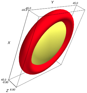
Figure 8: 3-D isodensity plot of the dense torus adopted for photoionization modelling of SuWt 2. The torus has a homogeneous density of 100 cm^-3, a radius of $38.1$ arcsec from its centre to the tube centre, and a tube radius of $6.9$ arcsec. The less dense oblate spheroid has a homogeneous density of 50 cm^-3, a semi-major axis of $31.2$ arcsec and a semi-minor axis of $6.9$ arcsec. Axis units are arcsec, where 1 arcsec is equal to $1.12\times 10^{-2}$ pc based on the distance determined by our photoionization models.

We used the 3 D photoionization code mocassin (version 2.02.67) to study the ring of the PN SuWt 2. The code, described in detail by Ercolano et al. (2003a, 2005, 2008), applies a Monte Carlo method to solve self-consistently the 3 D radiative transfer of the stellar and diffuse field in a gaseous and/or dusty nebula having asymmetric/symmetric density distribution and inhomogeneous/homogeneous chemical abundances, so it can deal with any structure and morphology. It also allows us to include multiple ionizing sources located in any arbitrary position in the nebula. It produces several outputs that can be compared with observations, namely a nebular emission-line spectrum, projected emission-line maps, temperature structure and fractional ionic abundances. This code has already been used for a number of axisymmetric PNe, such as NGC 3918 (Ercolano et al., 2003b), NGC 7009 (Gonçalves et al., 2006), NGC 6781 (Schwarz & Monteiro, 2006), NGC 6302 (Wright et al., 2011) and NGC 40 (Monteiro & Falceta-Gonçalves, 2011). To save computational time, we began with the gaseous model of a $22\times 22\times 3$ Cartesian grid, with the ionizing source being placed in a corner in order to take advantage of the axisymmetric morphology used. This initial low-resolution grid helped us explore the parameter space of the photoionization models, namely ionizing source, nebula abundances and distance. Once we found the best fitting model, the final simulation was done using a density distribution model constructed in $45\times 45\times 7$ cubic grids with the same size, corresponding to 14 175 cubic cells of length 1 arcsec each. Due to computational restrictions on time, we did not run any model with higher number of cubic cells. The atomic data set used for the photoionization modelling, includes the CHIANTI database (version 5.2; Landi et al., 2006), the improved coefficients of the H i, He i and He ii free–bound continuous emission (Ercolano & Storey, 2006) and the photoionization cross-sections and ionic ionization energies (Verner et al., 1993; Verner & Yakovlev, 1995).

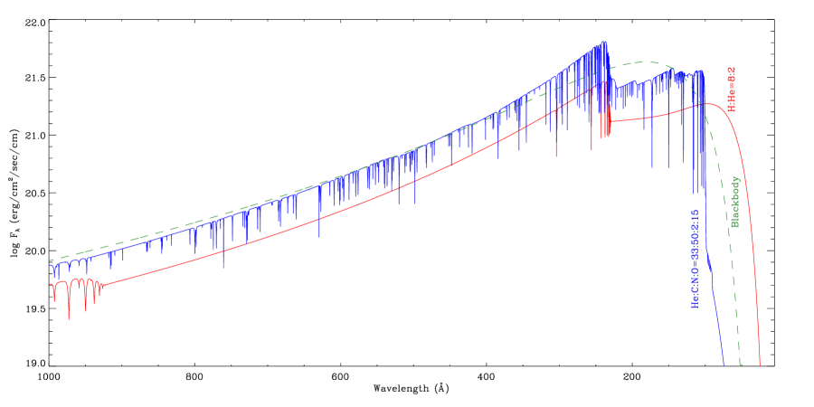
Figure 9: Comparison of two NLTE model atmosphere fluxes (Rauch, 2003) used as ionizing inputs in our two models. Red line: H-rich model with an abundance ratio of H : He = 8 : 2 by mass, $\log g=7$ (cgs) and $T_{\rm eff}=140\,000$ K. Blue line: PG 1159 model with He : C : N : O = 33 : 50 : 2 : 15, $\log g=7$ and $T_{\rm eff}=160\,000$ K. Dashed green line: the flux of a blackbody with $T_{\rm eff}=160\,000$ K.

The modelling procedure consists of an iterative process during which the calculated H$\beta$ luminosity $L_{{\rm H}\beta}$(erg s^-1), the ionic abundance ratios (i.e. He²⁺/He⁺, N⁺/H⁺, O²⁺/H⁺) and the flux intensities of some important lines, relative to H$\beta$ (such as He ii $\lambda$4686, $[$N ii$]$ $\lambda$6584 and $[$O iii$]$ $\lambda$5007) are compared with the observations. We performed a maximum of 20 iterations per simulation and the minimum convergence level achieved was 95%. The free parameters included distance and stellar characteristics, such as luminosity and effective temperature. Although we adopted the density and abundances derived in Sections 4 and 5, we gradually scaled up/down the abundances in Table LABEL:suwt2:tab:abundances:empirical until the observed emission-line fluxes were reproduced by the model. Due to the lack of infrared data we did not model the dust component of this object. We notice however some variations among the values of $c({\rm H}\beta)$ between the ring and the inner region in Table LABEL:suwt2:tab:obslines. It means that all of the observed reddening may not be due to the ISM. We did not include the outer bipolar lobes in our model, since the geometrical dilution reduces radiation beyond the ring. The faint bipolar lobes projected on the sky are far from the UV radiation field, and are dominated by the photodissociation region (PDR). There is a transition region between the photoionized region and PDR. Since mocassin cannot currently treat a PDR fully, we are unable to model the region beyond the ionization front, i.e. the ring. This low-density PN is extremely faint, and not highly optically thick (i.e. some UV radiations escape from the ring), so it is difficult to estimate a stellar luminosity from the total nebula H$\beta$ intrinsic line flux. The best-fitting model depends upon the effective temperature ($T_{\rm eff}$) and the stellar luminosity ($L_{\star}$), though both are related to the evolutionary stage of the central star. Therefore, it is necessary to restrict our stellar parameters to the evolutionary tracks of the post-AGB stellar models, e.g., ‘late thermal pulse’, ‘very late thermal pulse’ (VLTP), or ‘asymptotic giant branch final thermal pulse’ (see e.g. Iben & Renzini, 1983; Schönberner, 1983; Vassiliadis & Wood, 1994; Blöcker, 1995; Herwig, 2001; Miller Bertolami et al., 2006). To constrain $T_{\rm eff}$ and $L_{\star}$, we employed a set of evolutionary tracks for initial masses between $1$ and $7{\rm M}_{\bigodot}$ calculated by Blöcker (1995, Tables 3-5). Assuming a density model shown in Fig. 8, we first estimated the effective temperature and luminosity of the central star by matching the H$\beta$ luminosity $L({\rm H}\beta)$ and the ionic helium abundance ratio He²⁺/He⁺ with the values derived from observation and empirical analysis. Then, we scaled up/down abundances to get the best values for ionic abundance ratios and the flux intensities.

6.1 Model input parameters

6.1.1 Density distribution

The dense torus used for the ring was developed from the higher spectral resolution kinematic model of Jones et al. (2010) and our plasma diagnostics (Section 4). Although the density cannot be more than the low-density limit of $N_{\rm e}<100$ cm^-3 due to the [S ii] $\lambda\lambda$6716/6731 line ratio of $\gtrsim 1.40$, it was slightly adjusted to produce the total H$\beta$ Balmer intrinsic line flux $I({\rm H}\beta)$ derived for the ring and interior structure or the H$\beta$ luminosity $L({\rm H}\beta)=4\pi\,D^{2}\,I({\rm H}\beta)$ at the specified distance $D$. The three-dimensional density distribution used for the torus and interior structure is shown in Fig. 8. The central star is located in the centre of the torus. The torus has a radius of $38.1$ arcsec from its centre to the centre of the tube (1 arcsec is equal to $1.12\times 10^{-2}$ pc based on the best-fitting photoionization models). The radius of the tube of the ring is $6.9$ arcsec. The hydrogen number density of the torus is taken to be homogeneous and equal to $N_{\rm H}=100$ cm^-3. Smith et al. (2007) studied similar objects, including SuWt 2, and found that the ring itself can be a swept-up thin disc, and the interior of the ring is filled with a uniform equatorial disc. Therefore, inside the ring, there is a less dense oblate spheroid with a homogeneous density of 50 cm^-3, a semimajor axis of $31.2$ arcsec and a semiminor axis of $6.9$ arcsec. The H number density of the oblate spheroid is chosen to match the total $L({\rm H}\beta)$ and be a reasonable fit for H²⁺/H⁺ compared to the empirical results. The dimensions of the model were estimated from the kinematic model of Jones et al. (2010) with an adopted inclination of 68^∘. The distance was estimated over a range 2.1–2.7 kpc, which corresponds to a reliable range based on the H$\alpha$ surface brightness–radius relation of Frew & Parker (2006) and Frew (2008). The distance was allowed to vary to find the best-fitting model. The value of 2.3 kpc adopted in this work yielded the best match to the observed H$\beta$ luminosity and it is also in very good agreement with Exter et al. (2010).

6.1.2 Nebular abundances

All major contributors to the thermal balance of the gas were included in our model. We used a homogeneous elemental abundance distribution consisting of eight elements. The initial abundances of He, N, O, Ne, S and Ar were taken from the observed empirically derived total abundances listed in Table LABEL:suwt2:tab:abundances:empirical. The abundance of C was a free parameter, typically varying between $5\times 10^{-5}$ and $8\times 10^{-3}$ in PNe. We initially used the typical value of ${\rm C}/{\rm H}=5.5\times 10^{-4}$ (Kingsburgh & Barlow, 1994), and adjusted it to preserve the thermal balance of the nebula. We kept the initial abundances fixed while the stellar parameters and distance were being scaled to produce the best fit for the H$\beta$ luminosity and He²⁺/He⁺ ratio, and then we gradually varied them to obtain the finest match between the predicted and observed emission-line fluxes, as well as ionic abundance ratios from the empirical analysis.

The flux intensity of He ii $\lambda$4686 Å and the He²⁺/He⁺ ratio highly depend on the temperature and luminosity of the central star. Increasing either $T_{\rm eff}$ or $L_{\star}$ or both increases the He²⁺/He⁺ ratio. Our method was to match the He²⁺/He⁺ ratio, and then scale the He/H abundance ratio to produce the observed intensity of He ii $\lambda$4686 Å.

The abundance ratio of oxygen was adjusted to match the intensities of $[$O iii$]$ $\lambda\lambda$4959,5007 and to a lesser degree $[$O ii$]$ $\lambda\lambda$3726, 3729. In particular, the intensity of the $[$O ii$]$ doublet is unreliable due to the contribution of recombination and the uncertainty of about 30% at the extreme blue of the WiFeS. So we gradually modified the abundance ratio O/H until the best match for $[$O iii$]$ $\lambda\lambda$4959,5007 and O²⁺/H⁺ was produced. The abundance ratio of nitrogen was adjusted to match the intensities of $[$N ii$]$ $\lambda\lambda$6548,6584 and N⁺/H⁺. Unfortunately, the weak $[$N ii$]$ $\lambda$5755 emission line does not have a high S/N ratio in our data.

The abundance ratio of sulphur was adjusted to match the intensities of $[$S iii$]$ $\lambda$9069. The intensities of $[$S ii$]$ $\lambda\lambda$6716,6731 and S⁺/H calculated by our models are about seven and ten times lower than those values derived from observations and empirical analysis, respectively. The intensity of $[$S ii$]$ $\lambda\lambda$6716,6731 is largely increased due to shock-excitation effects.

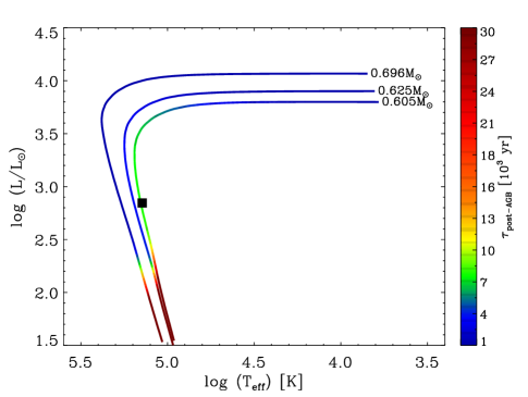
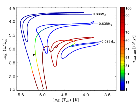
Figure 10: Hertzsprung–Russell diagrams for hydrogen-burning models (left-hand panel) with $(M_{\rm ZAMS},M_{\star})=$ $(3{\rm M}_{\bigodot},0.605{\rm M}_{\bigodot})$, $(3{\rm M}_{\bigodot},0.625{\rm M}_{\bigodot})$ and $(4{\rm M}_{\bigodot},0.696{\rm M}_{\bigodot})$, and helium-burning models (right-hand panel) with $(M_{\rm ZAMS},M_{\star})=$ $(1{\rm M}_{\bigodot},0.524{\rm M}_{\bigodot})$, $(3{\rm M}_{\bigodot},0.625{\rm M}_{\bigodot})$ and $(5{\rm M}_{\bigodot},0.836{\rm M}_{\bigodot})$ from Blöcker (1995) compared to the position of the central star of SuWt 2 derived from two different photoionization models, namely Model 1 (denoted by $\blacksquare$) and Model 2 ($\blacktriangledown$). On the right, the evolutionary tracks contain the first evolutionary phase, the VLTP (born-again scenario), and the second evolutionary phase. The colour scales indicate the post-AGB ages ($\tau_{\rm post-\textsc{agb}}$) in units of $10^{3}$ yr.

Finally, the differences between the total abundances from our photoionization model and those derived from our empirical analysis can be explained by the $icf$ errors resulting from a non-spherical morphology and properties of the exciting source. Gonçalves et al. (2012) found that additional corrections are necessary compared to those introduced by Kingsburgh & Barlow (1994) due to geometrical effects. Comparison with results from photoionization models shows that the empirical analysis overestimated the neon abundances. The neon abundance must be lower than the value found by the empirical analysis to reproduce the observed intensities of $[$Ne iii$]$ $\lambda\lambda$3869,3967. It means that the $icf$(Ne) of Kingsburgh & Barlow (1994) overestimates the unseen ionization stages. Bohigas (2008) suggested to use an alternative empirical method for correcting unseen ionization stages of neon. It is clear that with the typical Ne²⁺/Ne = O²⁺/O assumption of the $icf$ method, the neon total abundance is overestimated by the empirical analysis.

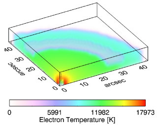
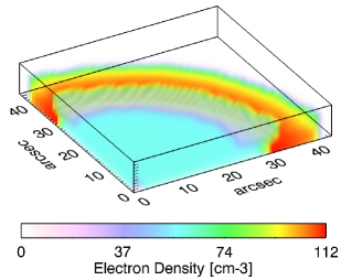
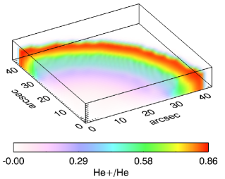
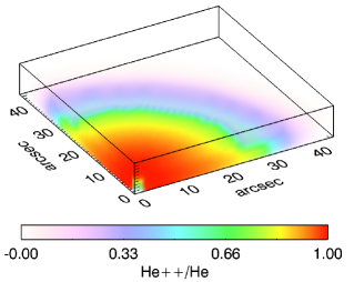
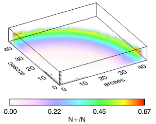
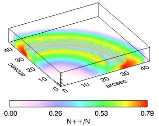
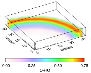
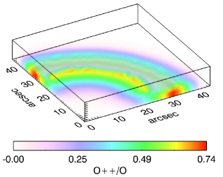
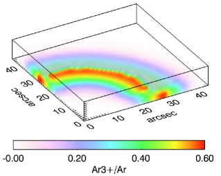
Figure 11: The 3 D distributions of electron temperature, electron density and ionic fractions from the adopted Model 2 constructed in $45\times 45\times 7$ cubic grids, and the ionizing source being placed in the corner (0,0,0). Each cubic cell has a length of $1.12\times 10^{-2}$ pc, which corresponds to the actual PN ring size.

6.1.3 Ionizing source

The central ionizing source of SuWt 2 was modelled using different non-local thermodynamic equilibrium (NLTE; Rauch, 2003) model atmospheres listed in Table LABEL:suwt2:tab:modelparameters, as they resulted in the best fit of the nebular emission-line fluxes. Initially, we tested a set of blackbody fluxes with the effective temperature ($T_{\rm eff}$) ranging from $80\,000$ to $190\,000$ K, the stellar luminosity compared to that of the Sun ($L_{\star}/{\rm L}_{\bigodot}$) ranging from 50-800 and different evolutionary tracks (Blöcker, 1995). A blackbody spectrum provides a rough estimate of the ionizing source required to photoionize the PN SuWt 2. The assumption of a blackbody spectral energy distribution (SED) is not quite correct as indicated by Rauch (2003). The strong differences between a blackbody SED and a stellar atmosphere are mostly noticeable at energies higher than 54 eV (He ii ground state). We thus successively used the NLTE Tübingen Model-Atmosphere Fluxes Package (TMAF; Rauch, 2003) for hot compact stars. We initially chose the stellar temperature and luminosity (gravity) of the best-fitting blackbody model, and changed them to get the best observed ionization properties of the nebula.

Fig. 9 shows the NTLE model atmosphere fluxes used to reproduce the observed nebular emission-line spectrum by our photoionization models. We first used a hydrogen-rich model atmosphere with an abundance ratio of H : He = 8 : 2 by mass, $\log g=7$ (cgs), and $T_{\rm eff}=140\,000$ K (Model 1), corresponding to the final stellar mass of $M_{\star}=0.605\,{\rm M}_{\bigodot}$ and the zero-age main sequence (ZAMS) mass of $M_{\rm\textsc{zams}}=3\,{\rm M}_{\bigodot}$, where ${\rm M}_{\bigodot}$ is the solar mass. However, its post-AGB age ($\tau_{\rm post-\textsc{agb}}$) of 7 500 yr, as shown in Fig. 10 (left-hand panel), is too short to explain the nebula’s age. We therefore moved to a hydrogen-deficient model, which includes Wolf-Rayet central stars ([WC]) and the hotter PG 1159 stars. [WC]-type central stars are mostly associated with carbon-rich nebula (Zijlstra et al., 1994). The evolutionary tracks of the VLTP for H-deficient models, as shown in Fig. 10 (right-hand panel), imply a surface gravity of $\log g=7.2$ for given $T_{\rm eff}$ and $L_{\star}$. From the high temperature and high surface gravity, we decided to use ‘typical’ PG 1159 model atmosphere fluxes (He : C : N : O = 33 : 50 : 2 : 15) with $T_{\rm eff}=160\,000$ K and $L_{\star}/{\rm L}_{\bigodot}=600$ (Model 2), corresponding to the post-AGB age of about $\tau_{\rm post-\textsc{agb}}=2$5 000 yr, $M_{\star}=0.64\,{\rm M}_{\bigodot}$ and $M_{\rm\textsc{zams}}=3\,{\rm M}_{\bigodot}$. The stellar mass found here is in agreement with the $0.7\,{\rm M}_{\bigodot}$ estimate of Exter et al. (2010). Fig. 9 compares the two model atmosphere fluxes with a blackbody with $T_{\rm eff}=160\,000$ K.

Table LABEL:suwt2:tab:modelparameters lists the parameters used for our final simulations in two different NTLE model atmosphere fluxes. The ionization structure of this nebula was best reproduced using these best two models. Each model has different effective temperature, stellar luminosity and abundances (N/H, O/H and Ne/H). The results of our two models are compared in Tables LABEL:suwt2:tab:modelresults–LABEL:suwt2:tab:ionratio to those derived from the observation and empirical analysis.

Table 8: Mean electron temperatures (K) weighted by ionic species for the whole nebula obtained from the photoionization model. For each element the upper row is for Model 1 and the lower row is for Model 2. The bottom lines present the mean electron temperatures and electron densities for the torus (ring) and the oblate spheroid (inside).

	Ion
Element	i	ii	iii	iv	v	vi	vii
H	11696	12904
	11470	12623
He	11628	12187	13863
	11405	11944	13567
C	11494	11922	12644	15061	17155	17236	12840
	11289	11696	12405	14753	16354	16381	12550
N	11365	11864	12911	14822	16192	18315	18610
	11170	11661	12697	14580	15836	17368	17475
O	11463	11941	12951	14949	15932	17384	20497
	11283	11739	12744	14736	15797	17559	19806
Ne	11413	11863	12445	14774	16126	18059	22388
	11196	11631	12215	14651	16166	18439	20488
S	11436	11772	12362	14174	15501	16257	18313
	11239	11557	12133	13958	15204	15884	17281
Ar	11132	11593	12114	13222	14908	15554	16849
	10928	11373	11894	13065	14713	15333	16392
	Torus				Spheroid
	$T_{\rm e}[$O iii$]$		$N_{\rm e}[$S ii$]$		$T_{\rm e}[$O iii$]$		$N_{\rm e}[$S ii$]$
M.1	12187 K		105 cm-3		15569 K		58 cm-3
M.2	11916 K		103 cm-3		15070 K		58 cm-3

Table 9: Fractional ionic abundances for SuWt 2 obtained from the photoionization models. For each element the upper row is for the torus (ring) and the lower row is for the oblate spheroid (inside).

		Ion
	Element	i	ii	iii	iv	v	vi	vii
Model 1	H	6.53($-2$)	9.35($-1$)
		3.65($-3$)	9.96($-1$)
	He	1.92($-2$)	7.08($-1$)	2.73($-1$)
		3.05($-4$)	1.27($-1$)	8.73($-1$)
	C	5.92($-3$)	2.94($-1$)	6.77($-1$)	2.33($-2$)	1.86($-4$)	7.64($-16$)	1.00($-20$)
		3.49($-5$)	1.97($-2$)	3.97($-1$)	4.50($-1$)	1.33($-1$)	1.09($-12$)	1.00($-20$)
	N	7.32($-3$)	4.95($-1$)	4.71($-1$)	2.62($-2$)	4.18($-4$)	6.47($-6$)	2.76($-17$)
		1.02($-5$)	1.30($-2$)	3.65($-1$)	3.97($-1$)	1.59($-1$)	6.69($-2$)	6.89($-13$)
	O	6.15($-2$)	4.98($-1$)	4.21($-1$)	1.82($-2$)	7.09($-4$)	1.34($-5$)	7.28($-8$)
		6.96($-5$)	1.26($-2$)	3.31($-1$)	4.03($-1$)	1.69($-1$)	6.00($-2$)	2.42($-2$)
	Ne	3.46($-4$)	6.70($-2$)	9.10($-1$)	2.26($-2$)	3.56($-4$)	4.25($-6$)	2.11($-9$)
		1.39($-6$)	3.32($-3$)	3.71($-1$)	3.51($-1$)	2.05($-1$)	6.55($-2$)	4.49($-3$)
	S	1.13($-3$)	1.67($-1$)	7.75($-1$)	5.52($-2$)	1.15($-3$)	6.20($-5$)	8.53($-7$)
		3.18($-6$)	3.89($-3$)	1.73($-1$)	3.53($-1$)	2.43($-1$)	1.57($-1$)	6.91($-2$)
	Ar	4.19($-4$)	3.15($-2$)	7.51($-1$)	2.10($-1$)	5.97($-3$)	1.13($-3$)	5.81($-5$)
		1.12($-7$)	2.33($-4$)	5.81($-2$)	2.83($-1$)	1.85($-1$)	2.73($-1$)	2.01($-1$)
Model 2	H	7.94($-2$)	9.21($-1$)
		4.02($-3$)	9.96($-1$)
	He	2.34($-2$)	7.25($-1$)	2.51($-1$)
		3.51($-4$)	1.33($-1$)	8.67($-1$)
	C	7.97($-3$)	3.23($-1$)	6.49($-1$)	1.93($-2$)	1.29($-4$)	5.29($-16$)	1.00($-20$)
		4.45($-5$)	2.23($-2$)	4.13($-1$)	4.41($-1$)	1.23($-1$)	1.00($-12$)	1.00($-20$)
	N	1.00($-2$)	5.44($-1$)	4.24($-1$)	2.15($-2$)	2.62($-4$)	2.20($-6$)	9.23($-18$)
		1.31($-5$)	1.52($-2$)	3.84($-1$)	4.07($-1$)	1.50($-1$)	4.40($-2$)	4.34($-13$)
	O	7.91($-2$)	5.29($-1$)	3.78($-1$)	1.40($-2$)	4.27($-4$)	2.05($-6$)	6.62($-11$)
		9.34($-5$)	1.50($-2$)	3.60($-1$)	4.20($-1$)	1.75($-1$)	2.97($-2$)	1.85($-4$)
	Ne	4.54($-4$)	7.35($-2$)	9.09($-1$)	1.73($-2$)	1.41($-4$)	1.94($-8$)	2.25($-14$)
		1.75($-6$)	3.85($-3$)	4.19($-1$)	3.86($-1$)	1.89($-1$)	1.73($-3$)	6.89($-7$)
	S	1.64($-3$)	1.95($-1$)	7.58($-1$)	4.47($-2$)	7.84($-4$)	3.39($-5$)	3.05($-7$)
		4.23($-6$)	4.86($-3$)	1.96($-1$)	3.61($-1$)	2.39($-1$)	1.47($-1$)	5.16($-2$)
	Ar	7.22($-4$)	3.99($-2$)	7.74($-1$)	1.81($-1$)	3.95($-3$)	5.62($-4$)	1.60($-5$)
		1.72($-7$)	3.22($-4$)	7.30($-2$)	3.30($-1$)	1.96($-1$)	2.62($-1$)	1.39($-1$)

Table 10: Integrated ionic abundance ratios for the entire nebula obtained from the photoionization models.

		Model 1		Model 2
Ionic ratio	Empirical	Abundance	Ionic Fraction	Abundance	Ionic Fraction
He+/H+	4.80($-2$)	5.308($-2$)	58.97%	5.419($-2$)	60.21%
He2+/H+	3.60($-2$)	3.553($-2$)	39.48%	3.415($-2$)	37.95%
C+/H+	–	9.597($-5$)	23.99%	1.046($-4$)	26.16%
C2+/H+	–	2.486($-4$)	62.14%	2.415($-4$)	60.38%
N+/H+	1.309($-4$)	9.781($-5$)	40.09%	1.007($-4$)	43.58%
N2+/H+	–	1.095($-4$)	44.88%	9.670($-5$)	41.86%
N3+/H+	–	2.489($-5$)	10.20%	2.340($-5$)	10.13%
O+/H+	1.597($-4$)	1.048($-4$)	40.30%	1.201($-4$)	42.44%
O2+/H+	1.711($-4$)	1.045($-4$)	40.20%	1.065($-4$)	37.64%
O3+/H+	–	2.526($-5$)	9.72%	2.776($-5$)	9.81%
Ne+/H+	–	6.069($-6$)	5.47%	6.571($-6$)	5.92%
Ne2+/H+	1.504($-4$)	8.910($-5$)	80.27%	9.002($-5$)	81.10%
Ne3+/H+	–	1.001($-5$)	9.02%	1.040($-5$)	9.37%
S+/H+ a	2.041($-6$)	2.120($-7$)	13.50%	2.430($-7$)	15.48%
S2+/H+	1.366($-6$)	1.027($-6$)	65.44%	1.013($-6$)	64.55%
S3+/H+	–	1.841($-5$)	11.73%	1.755($-7$)	11.18%
Ar+/H+	–	3.429($-8$)	2.54%	4.244($-8$)	3.14%
Ar2+/H+	1.111($-6$)	8.271($-7$)	61.26%	8.522($-7$)	63.13%
Ar3+/H+	4.747($-7$)	3.041($-7$)	22.52%	2.885($-7$)	21.37%
Ar4+/H+	–	5.791($-8$)	4.29%	5.946($-8$)	4.40%
Ar5+/H+	–	7.570($-8$)	5.61%	7.221($-8$)	5.35%

^a Shock excitation largely enhances the S⁺/H⁺ ionic abundance ratio.

6.2 Model results

6.2.1 Emission-line fluxes

Table LABEL:suwt2:tab:modelresults compares the flux intensities calculated by our models with those from the observations. The fluxes are given relative to H$\beta$, on a scale where H$\beta=100$. Most predicted line fluxes from each model are in fairly good agreement with the observed values and the two models produce very similar fluxes for most observed species. There are still some discrepancies in the few lines, e.g. $[$O ii$]$ $\lambda\lambda$3726,3729 and $[$S ii$]$ $\lambda\lambda$6716,6731. The discrepancies in $[$O ii$]$ $\lambda\lambda$3726,3729 can be explained by either recombination contributions or intermediate phase caused by a complex density distribution (see e.g. discussion in Ercolano et al., 2003c). $[$S ii$]$ $\lambda\lambda$6716,6731 was affected by shock-ionization and its true flux intensity is much lower without the shock fronts. Meanwhile, $[$Ar iii$]$ 7751 was enhanced by the telluric line. The recombination line H$\delta$ $\lambda$4102 and He ii $\lambda$5412 were also blended with the O ii recombination lines. There are also some recombination contributions in the $[$O ii$]$ $\lambda\lambda$7320,7330 doublet. Furthermore, the discrepancies in the faint auroral line [N ii] $\lambda$5755 and [O iii] $\lambda$4363 can be explained by the recombination excitation contribution (see section 3.3 in Liu et al., 2000).

6.2.2 Temperature structure

Table LABEL:suwt2:tab:temperatures represents mean electron temperatures weighted by ionic abundances for Models 1 and 2, as well as the ring region and the inside region of the PN. We also see each ionic temperature corresponding to the temperature-sensitive line ratio of a specified ion. The definition for the mean temperatures was given in Ercolano et al. (2003b); and in detail by Harrington et al. (1982). Our model results for $T_{\rm e}[$O iii$]$ compare well with the value obtained from the empirical analysis in § 4. Fig. 11 (top left) shows $T_{\rm e}$ obtained for Model 2 (adopted best-fitting model) constructed in $45\times 45\times 7$ cubic grids, and with the ionizing source being placed in the corner. It replicates the situation where the inner region has much higher $T_{\rm e}$ in comparison to the ring $T_{\rm e}$ as previously found by plasma diagnostics in § 4. In particular the mean values of $T_{\rm e}[$O iii$]$ for the ring (torus of the actual nebula) and the inside (spheroid) regions are around $12\,000$ and $15\,000$ K in all two models, respectively. They can be compared to the values of Table LABEL:suwt2:tab:tenediagnostics that is $T_{\rm e}[$O iii$]=12\,300$ K (ring) and $\lesssim 20\,000$ K (interior). Although the average temperature of $T_{\rm e}[$N ii$]\simeq 11\,700$ K over the entire nebula is higher than that given in Table LABEL:suwt2:tab:tenediagnostics, the average temperature of $T_{\rm e}[$O iii$]\simeq 13,000$ K is in decent agreement with that found by our plasma diagnostics.

It can be seen in Table LABEL:suwt2:tab:tenediagnostics that the temperatures for the two main regions of the nebula are very different, although we assumed a homogeneous elemental abundance distribution for the entire nebula relative to hydrogen. The temperature variations in the model can also be seen in Fig. 11. The gas density structure and the location of the ionizing source play a major role in heating the central regions, while the outer regions remain cooler as expected. Overall, the average electron temperature of the entire nebula increases by increasing the helium abundance and decreasing the oxygen, carbon and nitrogen abundances, which are efficient coolants. We did not include any dust grains in our simulation, although we note that a large dust-to-gas ratio may play a role in the heating of the nebula via photoelectric emissions from the surface of grains.

6.2.3 Ionization structure

Results for the fractional ionic abundances in the ring (torus) and inner (oblate spheroid) regions of our two models are shown in Table LABEL:suwt2:tab:ionfraction and Fig. 11. It is clear from the figure and table that the ionization structures from the models vary through the nebula due to the complex density and radiation field distribution in the gas. As shown in Table LABEL:suwt2:tab:ionfraction , He²⁺/He is much higher in the inner regions, while He⁺/He is larger in the outer regions, as expected. Similarly, we find that the higher ionization stages of each element are larger in the inner regions. From Table LABEL:suwt2:tab:ionfraction we see that hydrogen and helium are both fully ionized and neutrals are less than 8% by number in these best-fitting models. Therefore, our assumption of $icf({\rm He})=1$ is correct in our empirical method.

Table LABEL:suwt2:tab:ionratio lists the nebular average ionic abundance ratios calculated from the photoionization models. The values that our models predict for the helium ionic ratio are fairly comparable with those from the empirical methods given in § 5, though there are a number of significant differences in other ions. The O⁺/H⁺ ionic abundance ratio is about 33 per cent lower, while O²⁺/H⁺ is about 60% lower in Model 2 than the empirical observational value. The empirical value of S⁺ differs by a factor of 8 compared to our result in Model 2, explained by the shock-excitation effects on the $[$S ii$]$ $\lambda\lambda$6716,6731 doublet. Additionally, the Ne²⁺/H⁺ ionic abundance ratio was underestimated by roughly 67% in Model 2 compared to observed results, explained by the properties of the ionizing source. The Ar³⁺/H⁺ ionic abundance ratio in Model 2 is 56% lower than the empirical results. Other ionic fractions do not show major discrepancies; differences remain below 35%. We note that the N⁺/N ratio is roughly equal to the O⁺/O ratio, similar to what is generally assumed in the $icf$(N) method. However, the Ne²⁺/Ne ratio is nearly a factor of 2 larger than the O²⁺/O ratio, in contrast to the general assumption for $icf$(Ne) (see equation 5). It has already been noted by Bohigas (2008) that an alternative ionization correction method is necessary for correcting the unseen ionization stages for the neon abundance.

6.2.4 Evolutionary tracks

In Fig. 10 we compared the values of the effective temperature $T_{\rm eff}$ and luminosity $L_{\star}$ obtained from our two models listed in Table LABEL:suwt2:tab:modelparameters to evolutionary tracks of hydrogen-burning and helium-burning models calculated by Blöcker (1995). We compared the post-AGB age of these different models with the dynamical age of the ring found in § 3. The kinematic analysis indicates that the nebula was ejected about 23 400–26 300 yr ago. The post-AGB age of the hydrogen-burning model (left-hand panel in Fig. 10) is considerably shorter than the nebula’s age, suggesting that the helium-burning model (VLTP; right-hand panel in Fig. 10) may be favoured to explain the age.

The physical parameters of the two A-type stars also yield a further constraint. The stellar evolutionary tracks of the rotating models for solar metallicity calculated by Ekström et al. (2012) imply that the A-type stars, both with masses close to $2.7{\rm M}_{\bigodot}$ and $T_{\rm eff}\simeq 9200$ K, have ages of $\sim 500$ Myr. We see that they are in the evolutionary phase of the “blue hook”; a very short-lived phase just before the Hertzsprung gap. Interestingly, the initial mass of $3{\rm M}_{\bigodot}$ found for the ionizing source has the same age. As previously suggested by Exter et al. (2010), the PN progenitor with an initial mass slightly greater than $2.7{\rm M}_{\bigodot}$ can be coeval with the A-type stars, and it recently left the AGB phase. But, they adopted the system age of about 520 Myr according to the Y² evolutionary tracks (Yi et al., 2003; Demarque et al., 2004).

The effective temperature and stellar luminosity obtained for both models correspond to the progenitor mass of $3{\rm M}_{\bigodot}$. However, the strong nitrogen enrichment seen in the nebula is inconsistent with this initial mass, so another mixing process rather than the hot-bottom burning (HBB) occurs at substantially lower initial masses than the stellar evolutionary theory suggests for AGB-phase (Herwig, 2005; Karakas & Lattanzio, 2007; Karakas et al., 2009). The stellar models developed by Karakas & Lattanzio (2007) indicate that HBB occurs in intermediate-mass AGB stars with the initial mass of $\geqslant 5{\rm M}_{\bigodot}$ for the metallicity of $Z=0.02$; and $\geqslant 4{\rm M}_{\bigodot}$ for $Z=0.004$–$0.008$. However, they found that a low-metallicity AGB star ($Z=0.0001$) with the progenitor mass of $3{\rm M}_{\bigodot}$ can also experience HBB. Our determination of the argon abundance in SuWt 2 (see Table LABEL:suwt2:tab:modelparameters) indicates that it does not belong to the low-metallicity stellar population; thus, another non-canonical mixing process made the abundance pattern of this PN.

The stellar evolution also depends on the chemical composition of the progenitor, namely the helium content ($Y$) and the metallicity ($Z$), as well as the efficiency of convection (see e.g. Salaris & Cassisi, 2005). More helium increases the H-burning efficiency, and more metallicity makes the stellar structure fainter and cooler. Any change in the outer layer convection affects the effective temperature. There are other non-canonical physical processes such as rotation, magnetic field and mass-loss during Roche lobe overflow (RLOF) in a binary system, which significantly affect stellar evolution. Ekström et al. (2012) calculated a grid of stellar evolutionary tracks with rotation, and found that N/H at the surface in rotating models is higher than non-rotating models in the stellar evolutionary tracks until the end of the central hydrogen- and helium-burning phases prior to the AGB stage. The Modules for Experiments in Stellar Astrophysics (mesa) code developed by Paxton et al. (2011, 2013) indicates that an increase in the rotation rate (or angular momentum) enhances the mass-loss rate. The rotationally induced and magnetically induced mixing processes certainly influence the evolution of intermediate-mass stars, which need further studies by mesa. The mass-loss in a binary or even triple system is much more complicated than a single rotating star, and many non-canonical physical parameters are involved (see e.g. binstar code by Siess, 2006; Siess et al., 2013). Chen & Han (2002) used the Cambridge stellar evolution (stars) code developed by Eggleton (1971, 1972, 1973) to study numerically evolution of Population I binaries, and produced a helium-rich outer layer. Similarly, Benvenuto & De Vito (2003, 2005) developed a helium white dwarf from a low mass progenitor in a close binary system. A helium enrichment in the our layer can considerably influence other elements through the helium-burning mixing process.

7 Conclusion

In this paper we have analysed new optical integral-field spectroscopy of the PN SuWt 2 to study detailed ionized gas properties, and to infer the properties of the unobserved hot ionizing source located in the centre of the nebula. The spatially resolved emission-line maps in the light of $[$N ii$]$ $\lambda$6584 have described the kinematic structure of the ring. The previous kinematic model (Jones et al., 2010) allowed us to estimate the nebula’s age and large-scale kinematics in the Galaxy. An empirical analysis of the emission line spectrum led to our initial determination of the ionization structure of the nebula. The plasma diagnostics revealed as expected that the inner region is hotter and more excited than the outer regions of the nebula, and is less dense. The ionic abundances of He, N, O, Ne, S and Ar were derived based on the empirical methods and adopted mean electron temperatures estimated from the observed $[$O iii$]$ emission lines and electron densities from the observed $[$S ii$]$ emission lines.

We constructed photoionization models for the ring and interior of SuWt 2. This model consisted of a higher density torus (the ring) surrounding a low-density oblate spheroid (the interior disc). We assumed a homogeneous abundance distribution consisting of eight abundant elements. The initial aim was to find a model that could reproduce the flux intensities, thermal balance structure and ionization structure as derived from by the observations. We incorporated NLTE model atmospheres to model the ionizing flux of the central star. Using a hydrogen-rich model atmosphere, we first fitted all the observed line fluxes, but the time-scale of the evolutionary track was not consistent with the nebula’s age. Subsequently, we decided to use hydrogen-deficient stellar atmospheres implying a VLTP (born-again scenario), and longer time-scales were likely to be in better agreement with the dynamical age of the nebula. Although the results obtained by the two models of SuWt 2 are in broad agreement with the observations, each model has slightly different chemical abundances and very different stellar parameters. We found a fairly good fit to a hydrogen-deficient central star with a mass of $\sim 0.64{\rm M}_{\bigodot}$ with an initial (model) mass of $\sim 3{\rm M}_{\bigodot}$. The evolutionary track of Blöcker (1995) implies that this central star has a post-AGB age of about 25 000 yr. Interestingly, our kinematic analysis (based on $v_{\rm exp}$ from Jones et al., 2010) implies a nebular true age of about 23 400–26 300 yr.

Table LABEL:suwt2:tab:modelparameters lists two best-fitting photoionization models obtained for SuWt 2. The hydrogen-rich model atmosphere (Model 1) has a normal evolutionary path and yields a progenitor mass of $3{\rm M}_{\bigodot}$, a dynamical age of 7,500 yr and nebular ${\rm N}/{\rm O}=0.939$ (by number). The PG 1159 model atmosphere (Model 2) is the most probable solution, which can be explained by a VLTP phase or born-again scenario: VLTP $\rightarrow$ [WCL] $\rightarrow$ [WCE] $\rightarrow$ [WC]-PG 1159 $\rightarrow$PG 1159 (Blöcker, 2001; Herwig, 2001; Miller Bertolami & Althaus, 2006; Werner & Herwig, 2006). The PG 1159 model yields ${\rm N}/{\rm O}=0.816$ and a stellar temperature of $T_{\rm eff}=160$ kK corresponding to the progenitor mass of $3{\rm M}_{\bigodot}$ and much longer evolutionary time-scale. The VLTP can be characterized as the helium-burning model, but this cannot purely explain the fast stellar winds ($V_{\infty}=2000$ km s^-1) of typical [WCE] stars. It is possible that an external mechanism such as the tidal force of a companion and mass transfer to an accretion disc, or the strong stellar magnetic field of a companion can trigger (late) thermal pulses during post-AGB evolution.

The abundance pattern of SuWt 2 is representative of a nitrogen-rich PN, which is normally considered to be the product of a relatively massive progenitor star (Becker & Iben, 1980; Kingsburgh & Barlow, 1994). Recent work suggests that HBB, which enhances the helium and nitrogen, and decreases oxygen and carbon, occurs only for initial masses of $\geq$5 ${\rm M}_{\bigodot}$ ($Z=0.02$; Karakas & Lattanzio, 2007; Karakas et al., 2009); hence, the nitrogen enrichment seen in the nebula appears to result from an additional mixing process active in stars down to a mass of 3${\rm M}_{\bigodot}$. Additional physical processes such as rotation increase the mass-loss rate (Paxton et al., 2013) and nitrogen abundance at the stellar surface (end of the core H- and He-burning phases; Ekström et al., 2012). The mass-loss via RLOF in a binary (or triple) system can produce a helium-rich outer layer (Chen & Han, 2002; Benvenuto & De Vito, 2005), which significantly affects other elements at the surface.

References

- Aller & Liller (1968) Aller L. H., Liller W., 1968, Planetary Nebulae, Middlehurst B. M., Aller L. H., eds., the University of Chicago Press, p. 483
- Becker & Iben (1980) Becker S. A., Iben, Jr. I., 1980, ApJ, 237, 111
- Benvenuto & De Vito (2003) Benvenuto O. G., De Vito M. A., 2003, MNRAS, 342, 50
- Benvenuto & De Vito (2005) Benvenuto O. G., De Vito M. A., 2005, MNRAS, 362, 891
- Blöcker (1995) Blöcker T., 1995, A&A, 299, 755
- Blöcker (2001) Blöcker T., 2001, Ap&SS, 275, 1
- Bohigas (2008) Bohigas J., 2008, ApJ, 674, 954
- Bond (2000) Bond H. E., 2000, in Astronomical Society of the Pacific Conference Series, Vol. 199, Asymmetrical Planetary Nebulae II: From Origins to Microstructures, J. H. Kastner, N. Soker, & S. Rappaport, ed., p. 115
- Bond et al. (2002) Bond H. E., O’Brien M. S., Sion E. M., Mullan D. J., Exter K., Pollacco D. L., Webbink R. F., 2002, in Astronomical Society of the Pacific Conference Series, Vol. 279, Exotic Stars as Challenges to Evolution, C. A. Tout & W. van Hamme, ed., p. 239
- Bond et al. (2003) Bond H. E., Pollacco D. L., Webbink R. F., 2003, AJ, 125, 260
- Chen & Han (2002) Chen X., Han Z., 2002, MNRAS, 335, 948
- Demarque et al. (2004) Demarque P., Woo J.-H., Kim Y.-C., Yi S. K., 2004, ApJS, 155, 667
- Dopita et al. (2007) Dopita M., Hart J., McGregor P., Oates P., Bloxham G., Jones D., 2007, Ap&SS, 310, 255
- Dopita et al. (2010) Dopita M. et al., 2010, Ap&SS, 327, 245
- Dopita & Meatheringham (1990) Dopita M. A., Meatheringham S. J., 1990, ApJ, 357, 140
- Dopita & Meatheringham (1991) Dopita M. A., Meatheringham S. J., 1991, ApJ, 377, 480
- Dopita et al. (1996) Dopita M. A. et al., 1996, ApJ, 460, 320
- Eggleton (1971) Eggleton P. P., 1971, MNRAS, 151, 351
- Eggleton (1972) Eggleton P. P., 1972, MNRAS, 156, 361
- Eggleton (1973) Eggleton P. P., 1973, MNRAS, 163, 279
- Ekström et al. (2012) Ekström S. et al., 2012, A&A, 537, A146
- Ercolano et al. (2005) Ercolano B., Barlow M. J., Storey P. J., 2005, MNRAS, 362, 1038
- Ercolano et al. (2003a) Ercolano B., Barlow M. J., Storey P. J., Liu X.-W., 2003a, MNRAS, 340, 1136
- Ercolano et al. (2003c) Ercolano B., Barlow M. J., Storey P. J., Liu X.-W., Rauch T., Werner K., 2003c, MNRAS, 344, 1145
- Ercolano et al. (2003b) Ercolano B., Morisset C., Barlow M. J., Storey P. J., Liu X.-W., 2003b, MNRAS, 340, 1153
- Ercolano & Storey (2006) Ercolano B., Storey P. J., 2006, MNRAS, 372, 1875
- Ercolano et al. (2008) Ercolano B., Young P. R., Drake J. J., Raymond J. C., 2008, ApJS, 175, 534
- Exter et al. (2003) Exter K., Bond H., Pollacco D., Dufton P., 2003, in IAU Symposium, Vol. 209, Planetary Nebulae: Their Evolution and Role in the Universe, S. Kwok, M. Dopita, & R. Sutherland, ed., p. 234
- Exter et al. (2010) Exter K., Bond H. E., Stassun K. G., Smalley B., Maxted P. F. L., Pollacco D. L., 2010, AJ, 140, 1414
- Frew (2008) Frew D. J., 2008, PhD thesis, Department of Physics, Macquarie University, NSW 2109, Australia
- Frew et al. (2013a) Frew D. J., Bojičić I. S., Parker Q. A., 2013a, MNRAS, 431, 2
- Frew et al. (2013b) Frew D. J., Bojičić I. S., Parker Q. A., Pierce M. J., Gunawardhana M. L. P., Reid W. A., 2013b, MNRAS, submitted, e-print: arXiv:1303.4555
- Frew & Parker (2006) Frew D. J., Parker Q. A., 2006, in IAU Symposium, Vol. 234, Planetary Nebulae in our Galaxy and Beyond, Barlow M. J., Méndez R. H., eds., pp. 49–54
- Gesicki & Zijlstra (2000) Gesicki K., Zijlstra A. A., 2000, A&A, 358, 1058
- Gonçalves et al. (2006) Gonçalves D. R., Ercolano B., Carnero A., Mampaso A., Corradi R. L. M., 2006, MNRAS, 365, 1039
- Gonçalves et al. (2012) Gonçalves D. R., Wesson R., Morisset C., Barlow M., Ercolano B., 2012, in IAU Symposium, Vol. 283, IAU Symposium, pp. 144–147
- Harrington et al. (1982) Harrington J. P., Seaton M. J., Adams S., Lutz J. H., 1982, MNRAS, 199, 517
- Herwig (2001) Herwig F., 2001, Ap&SS, 275, 15
- Herwig (2005) Herwig F., 2005, ARA&A, 43, 435
- Howarth (1983) Howarth I. D., 1983, MNRAS, 203, 301
- Howarth & Adams (1981) Howarth I. D., Adams S., 1981, Program EQUIB. University College London, (Wesson R., 2009, Converted to FORTRAN 90)
- Hummer & Storey (1987) Hummer D. G., Storey P. J., 1987, MNRAS, 224, 801
- Iben & Renzini (1983) Iben, Jr. I., Renzini A., 1983, ARA&A, 21, 271
- Jacoby et al. (2001) Jacoby G. H., Ferland G. J., Korista K. T., 2001, ApJ, 560, 272
- Jones et al. (2010) Jones D., Lloyd M., Mitchell D. L., Pollacco D. L., O’Brien T. J., Vaytet N. M. H., 2010, MNRAS, 401, 405
- Karakas & Lattanzio (2007) Karakas A., Lattanzio J. C., 2007, PASA, 24, 103
- Karakas et al. (2009) Karakas A. I., van Raai M. A., Lugaro M., Sterling N. C., Dinerstein H. L., 2009, ApJ, 690, 1130
- Kingsburgh & Barlow (1994) Kingsburgh R. L., Barlow M. J., 1994, MNRAS, 271, 257
- Landi et al. (2006) Landi E., Del Zanna G., Young P. R., Dere K. P., Mason H. E., Landini M., 2006, ApJS, 162, 261
- Liu et al. (2000) Liu X.-W., Storey P. J., Barlow M. J., Danziger I. J., Cohen M., Bryce M., 2000, MNRAS, 312, 585
- Markwardt (2009) Markwardt C. B., 2009, in Astronomical Society of the Pacific Conference Series, Vol. 411, Astronomical Data Analysis Software and Systems XVIII, Bohlender D. A., Durand D., Dowler P., eds., p. 251
- Miller Bertolami & Althaus (2006) Miller Bertolami M. M., Althaus L. G., 2006, A&A, 454, 845
- Miller Bertolami et al. (2006) Miller Bertolami M. M., Althaus L. G., Serenelli A. M., Panei J. A., 2006, A&A, 449, 313
- Monteiro & Falceta-Gonçalves (2011) Monteiro H., Falceta-Gonçalves D., 2011, ApJ, 738, 174
- Moré (1977) Moré J., 1977, in Numerical Analysis, Watson G. A., ed., Vol. vol. 630, Springer-Verlag: Berlin, p. 105
- Parker et al. (2005) Parker Q. A., Phillipps S., Pierce M., et al., 2005, MNRAS, 362, 689
- Paxton et al. (2011) Paxton B., Bildsten L., Dotter A., Herwig F., Lesaffre P., Timmes F., 2011, ApJS, 192, 3
- Paxton et al. (2013) Paxton B. et al., 2013, ArXiv e-print: 1301.0319
- Rauch (2003) Rauch T., 2003, A&A, 403, 709
- Reid et al. (2009) Reid M. J. et al., 2009, ApJ, 700, 137
- Reid & Parker (2010) Reid W. A., Parker Q. A., 2010, PASA, 27, 187
- Roeser et al. (2010) Roeser S., Demleitner M., Schilbach E., 2010, AJ, 139, 2440
- Salaris & Cassisi (2005) Salaris M., Cassisi S., 2005, Evolution of Stars and Stellar Populations
- Schönberner (1983) Schönberner D., 1983, ApJ, 272, 708
- Schwarz et al. (1992) Schwarz H. E., Corradi R. L. M., Melnick J., 1992, A&AS, 96, 23
- Schwarz & Monteiro (2006) Schwarz H. E., Monteiro H., 2006, ApJ, 648, 430
- Seaton (1979a) Seaton M. J., 1979a, MNRAS, 187, 785
- Seaton (1979b) Seaton M. J., 1979b, MNRAS, 187, 73P
- Siess (2006) Siess L., 2006, A&A, 448, 717
- Siess et al. (2013) Siess L., Izzard R. G., Davis P. J., Deschamps R., 2013, A&A, 550, A100
- Smith et al. (2007) Smith N., Bally J., Walawender J., 2007, AJ, 134, 846
- Smits (1996) Smits D. P., 1996, MNRAS, 278, 683
- Steffen & López (2006) Steffen W., López J. A., 2006, RMxAA, 42, 99
- Storey & Hummer (1995) Storey P. J., Hummer D. G., 1995, MNRAS, 272, 41
- Tylenda et al. (2003) Tylenda R., Siódmiak N., Górny S. K., Corradi R. L. M., Schwarz H. E., 2003, A&A, 405, 627
- van Dokkum (2001) van Dokkum P. G., 2001, PASP, 113, 1420
- Vassiliadis & Wood (1994) Vassiliadis E., Wood P. R., 1994, ApJS, 92, 125
- Verner & Yakovlev (1995) Verner D. A., Yakovlev D. G., 1995, A&AS, 109, 125
- Verner et al. (1993) Verner D. A., Yakovlev D. G., Band I. M., Trzhaskovskaya M. B., 1993, Atomic Data and Nuclear Data Tables, 55, 233
- Werner & Herwig (2006) Werner K., Herwig F., 2006, PASP, 118, 183
- Wesson et al. (2012) Wesson R., Stock D. J., Scicluna P., 2012, MNRAS, 422, 3516
- West (1976) West R. M., 1976, PASP, 88, 896
- Wright et al. (2011) Wright N. J., Barlow M. J., Ercolano B., Rauch T., 2011, MNRAS, 418, 370
- Yi et al. (2003) Yi S. K., Kim Y.-C., Demarque P., 2003, ApJS, 144, 259
- Zijlstra et al. (1994) Zijlstra A. A., van Hoof P. A. M., Chapman J. M., Loup C., 1994, A&A, 290, 228