Correlation Critical Exponents for the Six-Vertex Model

Abstract

The six-vertex model on a square lattice is “exactly solvable” because an exact formula for the free energy can be obtained by Bethe Ansatz. However, exact formulas for the correlations of local bulk observables, such as the orientation of the arrow at a given edge, are in general not available. In this paper we consider the isotropic “zero-field” six-vertex model at small $|\Delta|$. We derive the large-distance asymptotic formula of the arrow-arrow correlation, which displays a power law decay and an anomalous exponent. Our method is based on an interacting fermions representation of the six-vertex model and does not use any information obtained from the exact solution.

I Introduction

The six-vertex model on a square lattice is called “exactly solvable” because of the discovery in 1967 of the exact formula for the free energy (Lieb, 1967a, b, c; Sutherland, 1967; Lieb, 1967d; Yang, 1967; Sutherland et al., 1967). Since then, there has been an intense research activity on this model and its transfer matrix Lieb and Wu (1972); Baxter (1982); Reshetikhin (2010). That led to important results also for systems that are equivalent to the six-vertex model in an exact or approximate form Lieb and Wu (1972); Baxter (1982); den Nijs (1983).

Many properties of the six-vertex model are determined by a characteristic parameter, $\Delta$. It is of special interest the critical case $|\Delta|\leq 1$, in which the spectrum of the transfer matrix was found to be gapless, and correlations of local bulk variables are therefore expected to display a large-distance power law decay. However, a direct study of correlations that validates this prediction has been in general very problematic.

In the simpler $\Delta=0$ case, in which the six-vertex model is a free fermion system, Sutherland Sutherland (1968) derived an exact formula for the arrow-arrow correlation which displayed staggered prefactors and power law decay. In the general $\Delta\neq 0$ case, except for the case of some non-local variables (Colomo and Pronko, 2012) and except for the non-critical regime $\Delta<-1$ (Jimbo and Miwa, 1995), exact formulas for correlations are not known. Nonetheless, large-distance properties of the arrow-arrow correlations have been inferred (Youngblood et al., 1980) on the basis of two equivalences: a) the transfer matrices of the six-vertex model and of the Heisenberg quantum chain commute McCoy and Wu (1968), hence the correlation of arrows placed along the same lattice line must coincide with the $S^{z}$-spin correlation of the Heisenberg model; b) the Heisenberg quantum chain is in the Luttinger Liquid universality class (Luther and Peschel, 1975; Fogedby, 1978; Haldane, 1980; Benfatto et al., 2010) (or can be studied via conformal field theory Bogoliubov et al. (1987)) and that fixes the power law decay of correlations.

More recently, a different method has been introduced to describe the critical phases of the six-vertex model, the Coulomb Gas picture for the height variable (Nienhuis, 1984). However, it appears that no specific result that can be compared with (Youngblood et al., 1980)’s analysis has been derived along this route.

In this paper we consider the isotropic zero-field six-vertex model and derive large distance asymptotic formulas for arrow-arrow correlations at small $|\Delta|$. Remarkably, our formulas are compatible with the features predicted in (Youngblood et al., 1980), including the occurrence of an anomalous critical exponent. Our approach is made of three steps. First we recast the model into an interacting dimers model following Baxter (1972); then we transform the dimer problem into a interacting fermions systems; finally, we study fermion correlations by the standard Renormalization Group techniques used in condensed matter theory Solyom (1979); Metzner and Di Castro (1993); Giamarchi (2004). Although this way of dealing with the six-vertex model was already suggested in Falco (2013), we observe that the technical implementation of the idea is new: the dimer interaction obtained from the six-vertex model equivalence turns out to be staggered, hence a different fermion representation, with different symmetries, is used. We also stress that our approach does not need any result from the exact solution.

II Definitions and Results

Consider a finite square lattice $\Lambda^{\prime}$. A configuration $\omega$ of the six-vertex model is obtained by drawing an arrow per each edge of the lattice so that the number of incoming arrow at each vertex is $2$ (the ice-rule). At each vertex there is one of the six possible arrangements of arrows in Fig. 1: assign them positive weights $p_{1},p_{2},\ldots,p_{6}$.

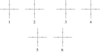
Figure 1: The six-possible configurations of arrows.

If $n_{j}(\omega)$ is the number of vertex in the configuration $\omega$ that display the arrangement number $j$, the partition function of the six vertex model is

$$Z=\sum_{\omega}\prod_{j=1}^{6}p_{j}^{n_{j}(\omega)}\;.$$

We assume periodic boundary condition, so that $n_{5}(\omega)=n_{6}(\omega)$ and $p_{5}p_{6}$ counts as one free parameter. Our results –as well as the analysis in (Youngblood et al., 1980)– are for the zero-field six-vertex model, i.e. the case

$$p_{1}=p_{2}=a\qquad p_{3}=p_{4}=b\;;$$

furthermore, for sake of simplicity, in this paper we will only consider the isotropic case $a=b$. Without loss of generality, we can fix $p_{5}=a$ and parametrize $p_{6}=2ae^{\lambda}$, for a real $\lambda$. The characteristic parameter of the six vertex model is

$$\Delta=\frac{a^{2}+b^{2}-p_{5}p_{6}}{2ab}=1-e^{\lambda}\;.$$

The case $\Delta=0$ is the free fermion case. Our goal is to show that, at least for small $|\Delta|$, there are correlations with power law decay. We consider the arrow orientation observable. Let ${\bf v}_{0}$ and ${\bf v}_{1}$ be the two orthogonal vectors that span $\Lambda^{\prime}$; a point of the plane will be parametrized by ${\bf x}=x^{\prime}_{0}{\bf v}_{0}+x^{\prime}_{1}{\bf v}_{1}$. For $d$ a horizontal edge centered at a point ${\bf x}$, the horizontal arrow orientation $\sigma_{0}({\bf x})$ is equal to $1$ if the arrow along $d$ points to the right, otherwise it is equal to $-1$; similarly, for $d$ a vertical edge centered at a point ${\bf x}$, the vertical arrow orientation $\sigma_{1}({\bf x})$ is equal to $1$ if the arrow along $d$ points up, otherwise it is equal to $-1$. In the infinite lattice limit, the arrow correlations have the following large $|{\bf x}|$ asymptotic formula: for two vertical arrows

$${\langle}\sigma_{1}({\bf x}+{\bf y})\sigma_{1}({\bf y}){\rangle}\sim c_{0}\frac{{x^{\prime}}_{1}^{2}-{x^{\prime}}_{0}^{2}}{({x^{\prime}}_{0}^{2}+{x^{\prime}}_{1}^{2})^{2}}+c_{-}\frac{(-1)^{x^{\prime}_{0}+x^{\prime}_{1}}}{({x^{\prime}}_{0}^{2}+{x^{\prime}}_{1}^{2})^{\kappa_{-}}}\;,$$ (1)

for one horizontal and one vertical arrow

$${\langle}\sigma_{1}({\bf x}+{\bf y}) \sigma_{0}({\bf y}){\rangle}\sim c_{0}\frac{-2x^{\prime}_{0}x^{\prime}_{1}}{({x^{\prime}_{0}}^{2}+{x^{\prime}_{1}}^{2})^{2}}-c_{-}\frac{(-1)^{x^{\prime}_{0}-x^{\prime}_{1}}}{({x^{\prime}_{0}}^{2}+{x^{\prime}_{1}}^{2})^{\kappa_{-}}}\;.$$ (2)

Each of the two above formulas is made of two terms: the former term has the same power law decay of the $\Delta=0$ case; the latter term has a power law decay with an anomalous (i.e. $\Delta$-dependent) critical exponent $\kappa_{-}=1+O(\Delta)$ and a staggering prefactor $(-1)^{x^{\prime}_{0}+x^{\prime}_{1}}$ or $(-1)^{x^{\prime}_{0}-x^{\prime}_{1}}$; besides, $c_{0}$ and $c_{-}$ are $\frac{2}{\pi^{2}}+O(\Delta)$. Note that $x^{\prime}_{0}+x^{\prime}_{1}$ and $x^{\prime}_{0}-x^{\prime}_{1}$ are integers. As by-product of our approach, we can obtain a Feynman graphs representation of the expansion of $\kappa_{-}$ in powers of $\lambda$. For example, at first order

$$\kappa_{-}=1-\frac{2\lambda}{\pi}+O(\lambda^{2})\;;$$ (3)

therefore, if $\lambda$ is positive and small (i.e. $\Delta$ negative and small), then at large distances the latter terms in (1) and (2) dominate over the former ones. Formulas (1), (2) and (3) are the main result of this paper. For $\Delta=0$, (1) coincides with Sutherland’s exact solution, see (6) of Sutherland (1968). For $\Delta\neq 0$, (1), (2) and (3) as expected from (Youngblood et al., 1980), are in agreement with the asymptotic formulas for the $S^{z}$–spin correlations in the Heisenberg quantum chain (Luther and Peschel, 1975; Fogedby, 1978; Haldane, 1980; Benfatto et al., 2010).

As an application of this result, we consider the large distance behavior of the covariance of the height variable van Beijeren (1977). For ${\bf u}$ the center of a plaquette of $\Lambda^{\prime}$, $h({\bf u})$ is the integer variable such that: if ${\bf x}$ is the center of a vertical bond

$${\bf v}_{0}\cdot\nabla h({\bf x})\equiv h({\bf x}+\frac{1}{2}{\bf v}_{0})-h({\bf x}-\frac{1}{2}{\bf v}_{0})=\sigma_{1}({\bf x})\;;$$

if ${\bf x}$ is the center of a horizontal bond

$$-{\bf v}_{1}\cdot\nabla h({\bf x})\equiv h({\bf x}-\frac{1}{2}{\bf v}_{1})-h({\bf x}+\frac{1}{2}{\bf v}_{1})=\sigma_{0}({\bf x})\;.$$

Because of the ice rule, $h({\bf u})$ is a scalar potential defined up to a global constant. From (1) we find the large $|{\bf x}|$ asymptotic formula

$${\langle}\big{[}h({\bf x}+{\bf u})-h({\bf u})\big{]}^{2}{\rangle}\sim 2c_{0}\ln|{\bf x}|\;;$$ (4)

hence $h({\bf u})$ has the same large distance behavior of a free boson field in dimension two. It is remarkable that, because of the staggering prefactor, the latter term in (1) does not determine the leading term of (4) regardless of the sign of $\lambda$.

In the next sections we will derive (1), (2), (3); and we will show how to obtain the application (4).

III Interacting Fermions Picture

Our point of departure is the equivalence of the six-vertex model on the square lattice $\Lambda^{\prime}$ with an interacting dimers model (IDM) on a different square lattice $\Lambda$ (Baxter, 1972). A dimer configuration $\omega$ on $\Lambda$ is a collection of dimers covering some of the edges of $\Lambda$ with the constraint that every vertex of $\Lambda$ is covered by one, and only one, dimer. The general partition function of the IDM is

$$Z_{\lambda}=\sum_{\omega}\exp\Big{\{}\lambda\sum_{d,d^{\prime}\in\omega}v(d,d^{\prime})\Big{\}}$$ (5)

where: the first sum is over all the dimer configurations; the second sum is over any pair of dimers in the configuration $\omega$; finally, $\lambda$ is the dimers coupling constant and $v(d,d)$ is an interaction that we have to determine to have the equivalence with the six-vertex model. To do so, first embed $\Lambda^{\prime}$ into $\Lambda$ as showed in Fig. 2;

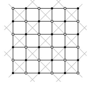
Figure 2: Superposition of the six-vertex lattice (in gray) and the interacting dimers lattice (in black). Note the role played by the bi-partition of the latter.

then use the mapping from the six-vertex configurations to the dimer configurations in Fig. 3.

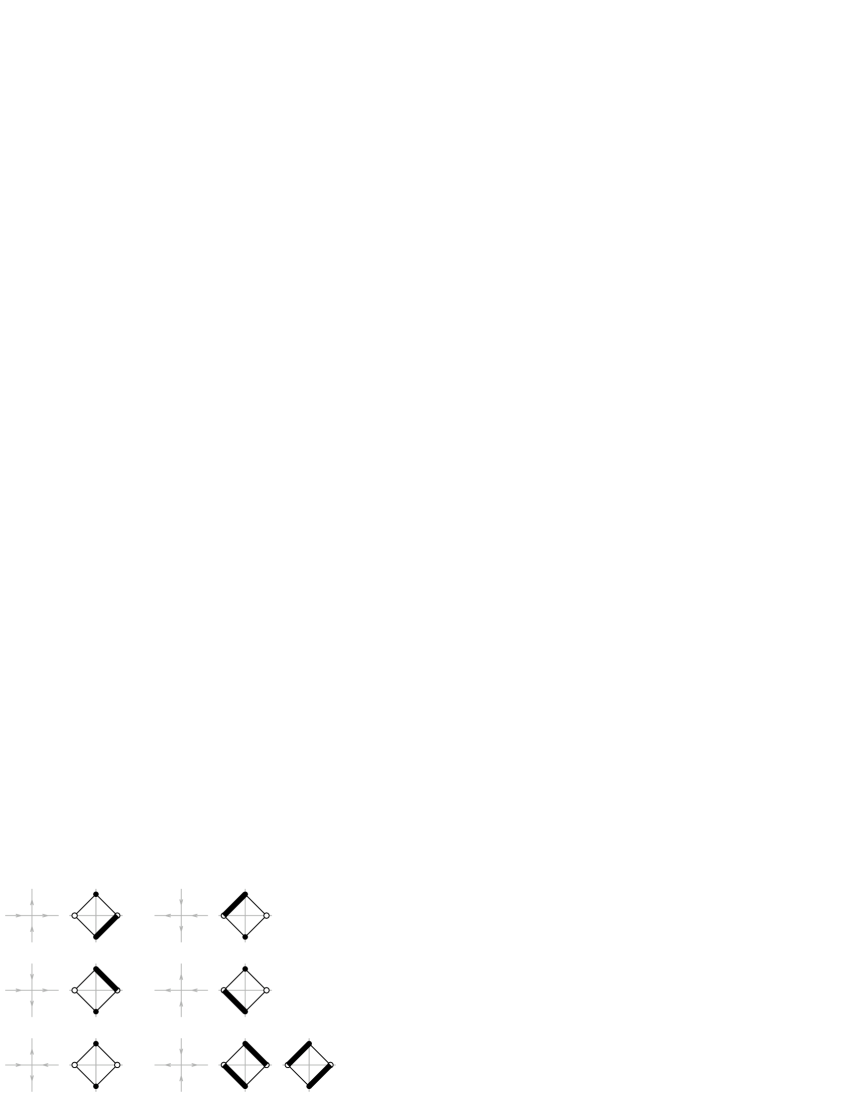
Figure 3: Map of the six-vertex configurations on $\Lambda^{\prime}$ into the dimer model configurations on $\Lambda$. The vertex configurations number $j=1,\ldots,5$ correspond to dimer arrangements with weight 1; the vertex configuration number 6 corresponds to two dimers arrangement, each of which with a weight $e^{\lambda}$. Note that in this Figure the black sites are in vertical position; when the black sites are in horizontal position all the dimer arrangements have to be counted with a weight 1.

As a consequence set $v(d,d^{\prime})=1$ if $d$ and $d^{\prime}$ are the two parallel nearest-neighbor dimers in the last two arrangement in Fig 3, which have the black sites in vertical positions; and $v(d,d^{\prime})=0$ otherwise. Let ${\bf e}_{0}$ and ${\bf e}_{1}$ the two vectors that span $\Lambda$; a point in the plane will be ${\bf x}=x_{0}{\bf e}_{0}+x_{1}{\bf e}_{1}$; in particular ${\bf v}_{0}={\bf e}_{0}-{\bf e}_{1}$ and ${\bf v}_{1}={\bf e}_{0}+{\bf e}_{1}$. A natural local bulk observable for the dimer model is the dimer occupancy $\nu_{j}({\bf x})$ which is equal to $1$ if the edge $\{{\bf x},{\bf x}+{\bf e}_{j}\}$ is occupied, and 0 otherwise. The relationships between the dimer occupancy and the arrow orientation of the equivalent six-vertex model is: for ${\bf x}$ a white site,

$$\sigma_{0}({\bf x}):=\nu_{0}({\bf x}-{\bf e}_{0})+\nu_{1}({\bf x})-\nu_{0}({\bf x})-\nu_{1}({\bf x}-{\bf e}_{1})$$ (6)

for ${\bf x}$ a black site,

$$\sigma_{1}({\bf x}):=\nu_{0}({\bf x})+\nu_{1}({\bf x})-\nu_{0}({\bf x}-{\bf e}_{0})-\nu_{1}({\bf x}-{\bf e}_{1})\;.$$ (7)

(As a side remark, also for the dimer model one can introduce an integer height function $H({\bf w})$ for every ${\bf w}$ that is the center of a plaquette of the lattice $\Lambda$. The standard definition is such that, if ${\bf u}$ is the center of a plaquette of $\Lambda^{\prime}$ and the center of a plaquette of $\Lambda$, one has

$$H({\bf u})=2h({\bf u})\;.$$

We will not need $H({\bf w})$ in the rest of the paper.) Since black and white lattice sites play a different role in the choice of the dimer potential, we need a fermion representation of the dimer model that takes into account the bi-partition of the square lattice. For this reason the fermion representation that we introduce below is different from the one used in (Falco, 2013).

Let ${\cal L}$ be the Bravais lattice of the black sites of $\Lambda$. ${\cal L}$ is spanned by the vectors ${\bf v}_{0}$ and ${\bf v}_{1}$; its primitive cell has volume $v_{P}=2$; and the reciprocal lattice of ${\cal L}$ is spanned by $\hat{\bf v}_{0}=\frac{1}{2}{\bf v}_{0}$ and $\hat{\bf v}_{1}=\frac{1}{2}{\bf v}_{1}$.

When $\lambda=0$ the dimer model is equivalent to a lattice fermion field without interaction. Namely

$$Z_{0}=\int\!D\psi\;\exp\Big{\{}-\sum_{{\bf x},{\bf y}\in{\cal L}}K_{{\bf x},{\bf y}}\psi^{+}_{\bf x}\psi^{-}_{{\bf y}+{\bf e}_{0}}\Big{\}}$$ (8)

where: $\{\psi^{+}_{\bf x},\psi^{-}_{{\bf x}+{\bf e}_{0}}:{\bf x}\in{\cal L}\}$ are Grassmann variables and $D\psi$ indicates the integration with respect to all of them; $K_{{\bf x},{\bf y}}$ is one of the possible Kasteleyn matrix for the square lattice dimer model

$$K_{{\bf x},{\bf y}}=\delta_{{\bf x},{\bf y}}-\delta_{{\bf x}-2{\bf e}_{0},{\bf y}}-\delta_{{\bf x}-{\bf e}_{0}+{\bf e}_{1},{\bf y}}-\delta_{{\bf x}-{\bf e}_{0}-{\bf e}_{1},{\bf y}}\;.$$

(8) is the partition function of a free fermion field, i.e. a Grassmann-valued Gaussian field with moment generator

$${\langle}e^{i\sum_{{\bf x}}(\psi^{+}_{\bf x}\eta^{-}_{\bf x}+\eta^{+}_{\bf x}\psi^{-}_{{\bf x}+{\bf e}_{0}})}{\rangle}_{0}=e^{\sum_{{\bf x},{\bf y}}S({\bf x}-{\bf y})\eta^{+}_{\bf x}\eta^{-}_{\bf y}}$$

where: the $\eta_{\bf x}$’s are external Grassmann variables; $S$ is the inverse Kasteleyn matrix

$$S({\bf x})=\frac{v_{P}}{2}\int_{\rm 1BZ}\!\frac{d{\bf k}}{(2\pi)^{2}}\;\frac{e^{i{\bf k}\cdot({\bf x}+{\bf e}_{0})}}{i\sin({\bf k}\cdot{\bf e}_{0})-\cos({\bf k}\cdot{\bf e}_{1})}$$

and 1BZ is the first Brillouin zone. The Fourier transform of $S$ has two poles at the Fermi momenta ${\bf k}=\omega{\bf p}_{F}$ for $\omega=\pm 1$ and ${\bf p}_{F}=(0,\frac{\pi}{2})$. Therefore, in view of the study of the scaling limit, it is convenient to decompose

$$S({\bf x})=\sum_{\omega=\pm}e^{i\omega{\bf p}_{F}\cdot{\bf x}}S_{\omega}({\bf x})$$

for

$$S_{\omega}({\bf x})=\frac{v_{P}}{2}\int_{\rm 1BZ}\!\frac{d{\bf k}}{(2\pi)^{2}}\;\frac{e^{i{\bf k}\cdot({\bf x}+{\bf e}_{0})}\chi({\bf k})}{i\sin({\bf k}\cdot{\bf e}_{0})-\omega\sin({\bf k}\cdot{\bf e}_{1})}$$

where $\chi({\bf k})$ is 1 in a neighborhood of ${\bf k}=0$ and such that $\chi({\bf k}-{\bf p}_{F})+\chi({\bf k}+{\bf p}_{F})=1$. Correspondingly, for $\varepsilon=\pm$,

$$\psi^{\varepsilon}_{{\bf x}} =\sum_{\omega}e^{i\varepsilon\omega{\bf p}_{F}\cdot{\bf x}}\psi_{{\bf x},\omega}^{\varepsilon}$$ (9)

where $(\psi^{+}_{{\bf x},+},\psi^{+}_{{\bf x},-})$ and $(\psi^{-}_{{\bf x},+},\psi^{-}_{{\bf x},-})^{T}$ are Dirac spinors with covariances

$${\langle}\psi_{{\bf x},\omega}^{+}\psi_{{\bf y},\omega^{\prime}}^{+}{\rangle}_{0}={\langle}\psi_{{\bf x}+{\bf e}_{0},\omega}^{-}\psi_{{\bf y}+{\bf e}_{0},\omega^{\prime}}^{-}{\rangle}_{0}=0$$

$${\langle}\psi_{{\bf x},\omega}^{+}\psi_{{\bf y}+{\bf e}_{0},\omega^{\prime}}^{-}{\rangle}_{0}=\delta_{\omega,\omega^{\prime}}S_{\omega}({\bf x}-{\bf y})\;.$$ (10)

If we now let $\lambda\neq 0$ one can verify that (5) becomes

$$Z_{\lambda}=Z_{0}{\langle}e^{(1-e^{\lambda})V(\psi)}{\rangle}_{0}$$ (11)

where $V(\psi)$ is quartic in the Grassmann variables with a simple explicit formula which is given in the next section. Besides, it is not difficult to find the leading term for large distances of the the dimer correlations: if $T$ indicates a truncated correlation and ${\bf z}={\bf x}-{\bf y}$, for two horizontal dimers

$${\langle}\nu_{0}({\bf x})\nu_{0}({\bf y}){\rangle}-{\langle}\nu_{0}({\bf x}){\rangle}{\langle}\nu_{0}({\bf y}){\rangle}$$

$$\sim(-1)^{z_{0}+z_{1}}\sum_{\omega}{\langle}\psi^{+}_{{\bf x},\omega}\psi^{-}_{{\bf x},\omega};\psi^{+}_{{\bf y},\omega}\psi^{-}_{{\bf y},\omega}{\rangle}^{T}$$

$$+(-1)^{z_{0}}\sum_{\omega}{\langle}\psi_{{\bf x},\omega}^{+}\psi^{-}_{{\bf x},-\omega};\psi_{{\bf y},-\omega}^{+}\psi^{-}_{{\bf y},\omega}{\rangle}^{T}\;,$$ (12)

whereas for one horizontal and one vertical dimer

$${\langle}\nu_{1}({\bf x})\nu_{0}({\bf y}){\rangle}-{\langle}\nu_{1}({\bf x}){\rangle}{\langle}\nu_{0}({\bf y}){\rangle}$$

$$\sim(-1)^{z_{0}+z_{1}}\sum_{\omega}i\omega{\langle}\psi^{+}_{{\bf x},\omega}\psi^{-}_{{\bf x},\omega};\psi^{+}_{{\bf y},\omega}\psi^{-}_{{\bf y},\omega}{\rangle}^{T}$$

$$+(-1)^{z_{0}}\sum_{\omega}i\omega{\langle}\psi_{{\bf x},\omega}^{+}\psi^{-}_{{\bf x},-\omega};\psi_{{\bf y},-\omega}^{+}\psi^{-}_{{\bf y},\omega}{\rangle}^{T}\;.$$ (13)

(The above formulas hold regardless of the colors of the sites ${\bf x}$ and ${\bf y}$.) The Renormalization Group argument that we will provide in the next section will indicate that to compute the correlations up to subleading terms, we can just replace the fields $\psi_{{\bf x},\omega}^{+}$, $\psi_{{\bf x},\omega}^{-}$ with the Thirring model fields $\psi_{\omega}^{\dagger}({\bf x})$, $\psi_{\omega}({\bf x})$ times a prefactor $2^{-\frac{1}{4}}e^{i\omega\frac{\pi}{8}}$ per each of them; from the exact solution of the Thirring model correlations Johnson (1961); Klaiber (1964); Hagen (1967); Falco (2006); Benfatto et al. (2007, 2009) (see also Falco (2012))

$${\langle}\psi^{\dagger}_{\omega}(0)\psi_{\omega}(0);\psi^{\dagger}_{\omega}({\bf x})\psi_{\omega}({\bf x}){\rangle}^{T}=c_{T,0}\frac{{x^{\prime}_{0}}^{2}-{x^{\prime}_{1}}^{2}-2i\omega x^{\prime}_{0}x^{\prime}_{1}}{({x^{\prime}_{0}}^{2}+{x^{\prime}_{1}}^{2})^{2}}$$

$${\langle}\psi_{\omega}^{\dagger}(0)\psi_{-\omega}(0);\psi_{-\omega}^{\dagger}({\bf x})\psi_{\omega}({\bf x}){\rangle}^{T}=\frac{c_{T,-}}{({x^{\prime}_{0}}^{2}+{x^{\prime}_{1}}^{2})^{\kappa_{-}}}$$ (14)

where the critical exponent $\kappa_{-}=1-\frac{\lambda_{T}}{2\pi}+O(\lambda_{T}^{2})$ and $\lambda_{T}$ is a parameter of the Thirring model: at first order $\lambda_{T}=4\lambda+O(\lambda^{2})$ (see next section).

IV RG Analysis

The fermion interaction $V(\psi)$ has explicit formula

$$\sum_{\omega_{1},\omega_{2}\atop\omega^{\prime}_{1},\omega^{\prime}_{2}}\frac{v_{P}^{4}}{(2\pi)^{7}}\int d{\bf k}_{1}d{\bf k}_{2}d{\bf q}_{1}d{\bf q}_{2}\;{\widehat{\psi}}_{{\bf k}_{1},\omega_{1}}^{+}{\widehat{\psi}}_{{\bf k}_{2},\omega_{2}}^{+}{\widehat{\psi}}_{{\bf q}_{1},\omega^{\prime}_{1}}^{-}{\widehat{\psi}}_{{\bf q}_{2},\omega^{\prime}_{2}}^{-}$$

$$\cdot\delta\left(\sum_{j=1}^{2}({\bf k}_{j}+\omega_{j}{\bf p}_{F})-\sum_{j=1}^{2}({\bf q}_{j}+\omega^{\prime}_{j}{\bf p}_{F})\right)v_{{\underline{\omega}};{\underline{\omega}}^{\prime}}(\underline{{\bf k}};\underline{{\bf q}})$$ (15)

where $v_{{\underline{\omega}};{\underline{\omega}}^{\prime}}(\underline{{\bf k}};\underline{{\bf q}})\equiv v_{\omega_{1},\omega_{2},\omega^{\prime}_{1},\omega^{\prime}_{2}}({\bf k}_{1},{\bf k}_{2},{\bf q}_{1},{\bf q}_{2})$ is

$$2\sin\left[({\bf k}_{1}-{\bf k}_{2})\frac{{\bf v}_{1}}{2}+(\omega_{1}-\omega_{2})\frac{\pi}{4}\right]$$

$$\cdot\sin\left[({\bf q}_{1}-{\bf q}_{2})\frac{{\bf v}_{0}}{2}-(\omega^{\prime}_{1}-\omega^{\prime}_{2})\frac{\pi}{4}\right]\;.$$ (16)

We follow the RG method in Gallavotti (1985). Integrating out the large momentum scales, we obtain an effective interaction

$$\sum_{n\geq 1}\sum_{\omega_{1}\ldots,\omega_{n}\atop\omega^{\prime}_{1}\ldots,\omega^{\prime}_{n}}\int\frac{d{\bf p}_{1}\cdots d{\bf q}_{n}}{(2\pi)^{4n-1}}\;{\widehat{\psi}}_{{\bf p}_{1},\omega_{1}}^{+}\cdots{\widehat{\psi}}_{{\bf p}_{n},\omega_{n}}^{+}{\widehat{\psi}}_{{\bf q}_{1},\omega^{\prime}_{1}}^{-}\cdots{\widehat{\psi}}_{{\bf q}_{n},\omega^{\prime}_{n}}^{-}$$

$$\cdot\delta\left(\sum_{j=1}^{n}({\bf p}_{j}+\omega_{j}{\bf p}_{F})-\sum_{j=1}^{n}({\bf q}_{j}+\omega^{\prime}_{j}{\bf p}_{F})\right){\widehat{w}}_{n;{\underline{\omega}};{\underline{\omega}}^{\prime}}(\underline{{\bf p}};\underline{{\bf q}})$$ (17)

where ${\widehat{w}}_{n;{\underline{\omega}};{\underline{\omega}}^{\prime}}$’s are series of Feynman graphs. Some symmetries are of crucial importance. For $R(k_{0},k_{1})=(k_{1},-k_{0})$, and $\vartheta(k_{0},k_{1})=(k_{1},k_{0})$, because of the explicit formulas of $v_{{\underline{\omega}};{\underline{\omega}}^{\prime}}(\underline{{\bf k}};\underline{{\bf q}})$ and of the Fourier transform of $S_{\omega}({\bf x})$, we have

$${\widehat{w}}_{n;{\underline{\omega}};{\underline{\omega}}^{\prime}}(\underline{R{\bf p}};\underline{R{\bf q}})=e^{i\frac{\pi}{2}\sum_{j}\omega_{j}}{\widehat{w}}_{n;{\underline{\omega}}^{\prime};{\underline{\omega}}}(\underline{{\bf q}};\underline{{\bf p}})$$

$${\widehat{w}}_{n;{\underline{\omega}};{\underline{\omega}}^{\prime}}(\underline{\vartheta{\bf p}};\underline{\vartheta{\bf q}})=e^{i\frac{\pi}{2}\sum_{j}\omega_{j}}{\widehat{w}}_{n;-{\underline{\omega}};-{\underline{\omega}}^{\prime}}(\underline{{\bf p}};\underline{{\bf q}})\;.$$ (18)

From power counting, there are two kinds of terms that are not irrelevant: the quartic and quadratic ones. Using (IV), the quartic terms give a local contribution

$$\lambda^{\prime}\sum_{{\bf x},\omega}\psi_{{\bf x},\omega}^{+}\psi_{{\bf x},\omega}^{-}\psi_{{\bf x},-\omega}^{+}\psi_{{\bf x},-\omega}^{-}$$ (19)

for $\lambda^{\prime}={\widehat{w}}_{2;+,-;-,+}(0,0;0,0)-{\widehat{w}}_{2;+,-;+,-}(0,0;0,0)=-4\lambda+O(\lambda^{\prime 2})$ the effective coupling constant. The quadratic terms cannot generate any local contribution of the form $\psi^{+}_{{\bf x},\omega}\psi^{-}_{{\bf x},-\omega}$ because of the delta function in (IV) and the fact that the momenta are small; therefore, using (IV), their only local contribution is

$$z\sum_{{\bf x},\omega}\psi_{{\bf x},\omega}^{+}\partial_{\omega}\psi_{{\bf x},\omega}^{-}\;,$$ (20)

for $z=\frac{1}{2}\left[-i\partial_{p_{0}}{\widehat{w}}_{1;+;+}({\bf p};{\bf p})-\partial_{p_{1}}{\widehat{w}}_{1;+;+}({\bf p};{\bf p})\right]_{{\bf p}=0}=O(\lambda^{2})$ the field renormalization counterterm and where $\partial_{\omega}$ is the Fourier transform of $ik_{0}-\omega k_{1}$. An important fact to note is that we have not included in (20) any mass term: the localization of the quadratic terms would give $m\sum_{{\bf x},\omega}\psi_{{\bf x},\omega}^{+}\psi_{{\bf x},\omega}^{-}$, for $m={\widehat{w}}_{1;\omega;\omega}(0;0)$; however, because of (IV), ${\widehat{w}}_{1;\omega;\omega}({\bf p};{\bf q})=i\omega{\widehat{w}}_{1;\omega;\omega}(R{\bf q};R{\bf p})$ and hence

$$m=0\;.$$

At infrared scales, the beta function of this fermion model asymptotically coincides with the beta function of the Thirring model, which is vanishing Metzner and Di Castro (1993). Hence, scaling each $\psi^{\varepsilon}_{{\bf x},\omega}$ of a factor $2^{-\frac{1}{4}}e^{i\omega\frac{\pi}{8}}$ so to match the standard normalization of the free part of the Thirring model, by comparison with Benfatto et al. (2007), we obtain $\lambda_{T}=-\lambda^{\prime}+O(\lambda^{2})$, where the higher orders are determined by the irrelevant terms.

V Height Covariance

For simplicity of notation we derive (4) in the case ${\bf u}=(-N-\frac{1}{2}){\bf v}_{0}+\frac{1}{2}{\bf v}_{1}$ and ${\bf x}=(2N+1){\bf v}_{0}$ only, but the formula for any ${\bf u}$ and ${\bf x}$ follows from the same argument. The height covariance is then given by

$$\sum_{i,j=-N}^{N}{\langle}{\bf v}_{0}\cdot\nabla h({\bf x}_{i})\;{\bf v}_{0}\cdot\nabla h({\bf x}_{j}){\rangle}\;,$$

where ${\bf x}_{j}=j{\bf v}_{0}+\frac{1}{2}{\bf v}_{1}$. In the double summation, the $O(N)$ term cancels Spencer : indeed since the summation of the height difference over any closed contour is vanishing by definition, and since the arrow correlation have a decay faster than the inverse distance, one can replace $j=-N,\ldots,N$ with $|j|\geq N+1$. Hence the height covariance becomes

$$-\sum_{|i|\leq N}\sum_{|j|\geq N+1}{\langle}\sigma_{1}({\bf x}_{i})\;\sigma_{1}({\bf x}_{j}){\rangle}\;.$$

Now plug (1) into this formula: the staggered term gives a contribution that is bounded in $N$, whereas the un-staggered one gives $2c_{0}\ln N$ plus terms that are bounded in $N$.

VI Conclusion

We have showed that the interacting fermions representation of the six-vertex model, in combination with a Renormalization Group approach, provides a precise formula for the large distance decay of the arrow-arrow correlations for small $|\Delta|$. More in general, using ideas in (Falco, 2006; Benfatto et al., 2007), one could show that the scaling limit of the $n$-points arrow correlations, apart from staggering prefactors, are linear combinations of Thirring model correlations.

References

- Lieb (1967a) E. Lieb, Phys. Rev. Lett. 18, 692 (1967a).
- Lieb (1967b) E. Lieb, Phys. Rev. 162, 162 (1967b).
- Lieb (1967c) E. Lieb, Phys. Rev. Lett. 18, 1046 (1967c).
- Sutherland (1967) B. Sutherland, Phys. Rev. Lett. 19, 103 (1967).
- Lieb (1967d) E. Lieb, Phys. Rev. Lett. 19, 108 (1967d).
- Yang (1967) C. Yang, Phys. Rev. Lett. 19, 586 (1967).
- Sutherland et al. (1967) B. Sutherland, C. Yang, and C. Yang, Phys. Rev. Lett. 19, 588 (1967).
- Lieb and Wu (1972) E. Lieb and F. Wu, in Phase transitions and critical phenomena, Vol. 1 (Academic press London, 1972).
- Baxter (1982) R. Baxter, Exactly solved models in statistical mechanics (Academic press London, 1982).
- Reshetikhin (2010) N. Reshetikhin, in Exact methods in low-dimensional statistical physics and quantum computing (Oxford Univ. Press, Oxford, 2010) pp. 197–266.
- den Nijs (1983) M. den Nijs, Phys. Rev. B 27, 1674 (1983).
- Sutherland (1968) B. Sutherland, Phys. Lett. A 26, 532 (1968).
- Colomo and Pronko (2012) F. Colomo and A. Pronko, Theor. Math. Phys. 171, 641 (2012).
- Jimbo and Miwa (1995) M. Jimbo and T. Miwa, Algebraic analysis of solvable lattice models, edited by AMS, Vol. 85 (Conference Board of the Mathematical Sciences, Washington, DC, 1995).
- Youngblood et al. (1980) R. Youngblood, J. Axe, and B. McCoy, Phys. Rev. B 21, 5212 (1980).
- McCoy and Wu (1968) B. McCoy and T. T. Wu, Il Nuovo Cimento B Series 10 56, 311 (1968).
- Luther and Peschel (1975) A. Luther and I. Peschel, Phys. Rev. B 12, 3908 (1975).
- Fogedby (1978) H. Fogedby, J. Phys. C 11, 4767 (1978).
- Haldane (1980) F. Haldane, Phys. Rev. Lett. 45, 1358 (1980).
- Benfatto et al. (2010) G. Benfatto, P. Falco, and V. Mastropietro, Phys. Rev. Lett. 104, 75701 (2010).
- Bogoliubov et al. (1987) N. Bogoliubov, A. Izergin, and N. Y. Reshetikhin, J. Phys A 20, 5361 (1987).
- Nienhuis (1984) B. Nienhuis, J. Stat. Phys. 34, 731 (1984).
- Baxter (1972) R. Baxter, Ann.Phys. 70, 193 (1972).
- Solyom (1979) J. Solyom, Adv. in Phys. 28, 201 (1979).
- Metzner and Di Castro (1993) W. Metzner and C. Di Castro, Phys. Rev. B 47, 16107 (1993).
- Giamarchi (2004) T. Giamarchi, Quantum physics in one dimension (Oxford University Press, USA, 2004).
- Falco (2013) P. Falco, Phys. Rev. E 87, 060101 (2013).
- van Beijeren (1977) H. van Beijeren, Phys. Rev. Lett. 38, 993 (1977).
- Johnson (1961) K. Johnson, N. Cimento , 773 (1961).
- Klaiber (1964) B. Klaiber, Helv. Phys. Acta 37, 554 (1964).
- Hagen (1967) C. Hagen, N. Cimento B 51, 169 (1967).
- Falco (2006) P. Falco, arXiv:hep-th/0703274 , PhD Thesis (2006).
- Benfatto et al. (2007) G. Benfatto, P. Falco, and V. Mastropietro, Comm. Math. Phys. 273, 67 (2007).
- Benfatto et al. (2009) G. Benfatto, P. Falco, and V. Mastropietro, Comm. Math. Phys. 285, 713 (2009).
- Falco (2012) P. Falco, arXiv:1208.6568 (2012).
- Gallavotti (1985) G. Gallavotti, Rev. Mod. Phys. 57, 471 (1985).
- (37) T. Spencer, Private communication.