Theory of wind accretion

Abstract

A review of wind accretion in high-mass X-ray binaries is presented. We focus attention to different regimes of quasi-spherical accretion onto the neutron star: the supersonic (Bondi) accretion, which takes place when the captured matter cools down rapidly and falls supersonically toward NS magnetospghere, and subsonic (settling) accretion which occurs when plasma remains hot until it meets the magnetospheric boundary. Two regimes of accretion are separated by an X-ray luminosity of about $4\times 10^{36}$ erg/s. In the subsonic case, which sets in at low luminosities, a hot quasi-spherical shell must be formed around the magnetosphere, and the actual accretion rate onto NS is determined by ability of the plasma to enter the magnetosphere due to Rayleigh-Taylor instability. We calculate the rate of plasma entry the magnetopshere and the angular momentum transfer in the shell due to turbulent viscosity appearing in the convective differentially rotating shell. We also discuss and calculate the structure of the magnetospheric boundary layer where the angular momentum between the rotating magnetosphere and the base of the differentially rotating quasi-spherical shell takes place. We show how observations of equilibrium X-ray pulsars Vela X-1 and GX 301-2 can be used to estimate dimensionless parameters of the subsonic settling accretion theory, and obtain the width of the magnetospheric boundary layer for these pulsars.

1 Introduction

In close binary systems, there can be two different regimes of accretion onto the compact object – disk accretion and quasi-spherical accretion. The disk accretion regime is usually realized when the optical star overfills its Roche lobe. Quasi-spherical accretion is most likely to occur in high-mass X-ray binaries (HMXB) when the optical star of early spectral class (O-B) does not fill its Roche lobe, but has a significant mass loss via stellar wind. We shall discuss the wind accretion regime, in which a bow shock forms in the stellar wind near the compact star. The structure of the bow shock and accretion wake is quite complicated and is non-stationary (see e.g. numerical simulations 1988ApJ…335..862F , 1999A&A…346..861R , 2004A&A…419..335N , among others). The characteristic distance at which the bow shock forms is about the Bondi radius $R_{B}=2GM/(v_{w}^{2}+v_{orb}^{2})$, where $v_{w}$ is the wind velocity (typically hundred-thousand km/s), $v_{orb}$ is the orbital velocity of the compact star. Here we shall consider accretion onto magnetized neutron stars (NS) observed as X-ray pulsars. The rate of gravitational capture of mass from the wind (the Bondi mass accretion rate) is $\dot{M}_{B}\simeq\rho_{w}R_{B}^{2}v_{w}$.

There can be two different cases of quasi-spherical accretion. The classical Bondi-Hoyle-Littleton accretion takes place when the shocked matter rapidly cools down (via Compton cooling), and the matter freely falls toward the NS magnetosphere. (see Fig. 2). A shock is formed at some distance above the magnetosphere. Above the magnetosphere, the shocked matter rapidly cools down and enters the magnetopshere via Rayleigh-Taylor instability 1976ApJ…207..914A . The magnetospheric boundary is characterized by the Alfvén radius $R_{A}$, which can be calculated from the balance of the ram pressure of the infalling matter and the magnetic field pressure at the boundary. The captured matter from the wind has a specific angular momentum $j_{w}\sim\omega_{B}R_{B}^{2}$ 1975A&A….39..185I . Depending on the sign of $j_{w}$ (prograde or retorgrade), the NS can spin-up or spin-down. This regime of quasi-sphericl accretion is realized in bright X-ray pulsars with $L_{x}>4\times 10^{36}$ erg/s 2012MNRAS.420..216S .

If the shocked matter remains hot (when plasma cooling time is much longer than the free-fall time, $t_{cool}\gg t_{ff}$), a hot quasi-static shell forms above the magnetosphere. The subsonic (settling) accretion sets in (see Fig. 2). In this case, both spin-up or spin-down of the NS is possible, even if the sign of $j_{w}$ is positive (prograde). The shell mediates the angular momentum transfer from the NS magnetosphere via viscous stresses due to convection (see below). In this regime, the mean radial velocity of matter in the shell $u_{r}$ is smaller than the free-fall velocity $u_{ff}$: $u_{r}=f(u)u_{ff}$, $f(u)<1$, and is determined by the palsma cooling rate near the magnetosphere (due to Compton or radiative cooling): $f(u)\sim[t_{ff}(R_{A})/t_{cool}(R_{A})]^{1/3}$. Here the actual mass accretion rate onto NS can be significantly smaller than the Bondi mass accretion rate, $\dot{M}=f(u)\dot{M}_{B}$. The settling accretion occurs at $L_{x}<4\times 10^{36}$ erg/s 2012MNRAS.420..216S .

Figure 1: Supersonic (Bondi-Hoyle-Littleton) accretion onto magnetized NS

Figure 2: Subsonic settling accretion onto magnetized NS

2 Vertical structure of the subsonic shell

In the quasi-steady state, the structure of the shell is described by hydrostatic equilibrium:

$$-\frac{1}{\rho}\frac{dP}{dR}-\frac{GM}{R^{2}}=0$$ (1)

with the adiabatic solution:

$$\frac{{\cal R}T}{\mu_{m}}=\left(\frac{\gamma-1}{\gamma}\right)\frac{GM}{R}\,.$$ (2)

(Turbulence in the shell can play a certain role in hydrostatic equilibrium; this complicates formulas but does not change the conclusions, see 2012MNRAS.420..216S for more detail). For $\gamma=5/3$ the density profile in the shell is:

$$\rho(R)=\rho(R_{A})\left(\frac{R_{A}}{R}\right)^{3/2}\,.$$ (3)

The Alfvén surface is found from the balance of gas pressure and the magnetic field pressure at the magnetopsheric boundary:

$$P_{g}=\frac{B^{2}(R_{A})}{8\pi}\,.$$ (4)

Taking into account the mass continuity equation in the settling regime, we obtain:

$$R_{A}=\left[\frac{4\gamma}{(\gamma-1)}f(u)K_{2}\frac{\mu^{2}}{\dot{M}\sqrt{2GM}}\right]^{2/7}\,.$$ (5)

Here $K_{2}\approx 7.6$ is the numerical coefficient which takes into account the enhancement of the magnetic field at the magnetopsheric boundary due to emerging currents 1976ApJ…207..914A .

The plasma enters the magnetosphere of the slowly rotating neutron star due to the Rayleigh-Taylor instability. The boundary between the plasma and the magnetosphere is stable at high temperatures $T>T_{cr}$, but becomes unstable at $T<T_{cr}$, and remains in a neutral equilibrium at $T=T_{cr}$ 1977ApJ…215..897E . The critical temperature is:

$${\cal R}T_{cr}=\frac{1}{2}\frac{\cos\chi}{\kappa R_{A}}\frac{\mu_{m}GM}{R_{A}}\,.$$ (6)

Here $\kappa$ is the local curvature of the magnetosphere, $\chi$ is the angle the outer normal makes with the radius-vector at a given point. The effective gravity acceleration can be written as

$$g_{eff}=\frac{GM}{R_{A}^{2}}\cos\chi\left(1-\frac{T}{T_{cr}}\right)\,.$$ (7)

The temperature in the quasi-static shell is given by (2), and the condition for the magnetosphere instability can thus be rewritten as:

$$\frac{T}{T_{cr}}=\frac{2(\gamma-1)}{\gamma}\frac{\kappa R_{A}}{\cos\chi}<1\,.$$ (8)

Let us consider the development of the interchange instability when cooling (predominantly Compton cooling) is present. The temperature changes as kompaneets56 , 1965PhFl….8.2112W

$$\frac{dT}{dt}=-\frac{T-T_{x}}{t_{C}}\,,$$ (9)

where the Compton cooling time is

$$t_{C}=\frac{3}{2\mu_{m}}\frac{\pi R_{A}^{2}m_{e}c^{2}}{\sigma_{T}L_{x}}\approx 10.6[\hbox{s}]R_{9}^{2}\dot{M}_{16}^{-1}\,.$$ (10)

Here $m_{e}$ is the electron mass, $\sigma_{T}$ is the Thomson cross section, $L_{x}=0.1\dot{M}c^{2}$ is the X-ray luminosity, $T$ is the electron temperature (which is equal to the ion temperature since the timescale of electron-ion energy exchange here is the shortest possible), $T_{x}$ is the X-ray temperature and $\mu_{m}=0.6$ is the molecular weight. The photon temperature is $T_{x}=(1/4)T_{cut}$ for a bremsstrahlung spectrum with an exponential cut-off at $T_{cut}$, typically $T_{x}=3-5$ keV. The solution of equation (9) reads:

$$T=T_{x}+(T_{cr}-T_{x})e^{-t/t_{C}}\,.$$ (11)

We note that $T_{cr}\sim 30\,\hbox{keV}\gg T_{x}\sim 3$ keV. It is seen that for $t\approx 2t_{C}$ the temperature decreases to $T_{x}$. In the linear approximation the temperature changes as:

$$T\approx T_{cr}(1-t/t_{C})\,.$$ (12)

Plugging this expression into (7), we find that the effective gravity acceleration increases linearly with time as:

$$g_{eff}\approx\frac{GM}{R_{A}^{2}}\frac{t}{t_{C}}\cos\chi\,.$$ (13)

Correspondingly, the velocity of matter due to the instability growth increases with time as:

$$u_{r}=\int\limits_{0}^{t}g_{eff}dt=\frac{GM}{R_{A}^{2}}\frac{t^{2}}{2t_{C}}\cos\chi\,.$$ (14)

Let us introduce the mean rate of the instability growth

$$<u_{i}>=\frac{\int udt}{t}=\frac{1}{6}\frac{GM}{R_{A}^{2}}\frac{t^{2}}{t_{C}}=\frac{1}{6}\frac{GM}{R_{A}^{2}t_{C}}\left(\frac{\zeta R_{A}}{<u_{i}>}\right)^{2}\,.$$ (15)

Here $\zeta\lesssim 1$ and $\zeta R_{A}$ is the characteristic scale of the instability that grows with the rate $<u_{i}>$. So for the mean rate of the instability growth in the linear stage we find

$$<u_{i}>=\left(\frac{\zeta^{2}GM}{6t_{C}}\right)^{1/3}=\frac{\zeta^{2/3}}{12^{1/3}}\sqrt{\frac{2GM}{R_{A}}}\left(\frac{t_{ff}}{t_{C}}\right)^{1/3}\,.$$ (16)

Here we have introduced the free-fall time as

$$t_{ff}=\frac{R_{A}^{3/2}}{\sqrt{2GM}}\,.$$ (17)

Therefore, the factor $f(u)$ becomes:

$$f(u)=\frac{<u_{i}>}{u_{ff}(R_{A})}\,.$$ (18)

Substituting (16) and (18) into (5), we find for the Alfven radius in this regime:

$$R_{A}\approx 1.37\times 10^{9}[\hbox{cm}]\left(\zeta\frac{\mu_{30}^{3}}{\dot{M}_{16}}\right)^{2/11}\,.$$ (19)

(We stress the difference of the obtained expression for the Alfven radius with the standard one, $R_{A}\sim\mu^{4/7}/\dot{M}^{-2/7}$). Plugging (19) into (18), we obtain explicit expression for $f(u)$:

$$f(u)\approx 0.22\zeta^{7/11}\dot{M}_{16}^{4/11}\mu_{30}^{-1/11}\,.$$ (20)

In principle, for moderately rotating X-ray puslars plasma can entry a rotating magnetosphere via Kelvin-Helmholtz instability 1983ApJ…266..175B :

$$u_{KH}\simeq 0.1\gamma_{KH}/k=0.1\left\{\begin{array}[]{cc}u_{\phi}\frac{\sqrt{\rho_{i}/\rho_{e}}}{1+\rho_{i}/\rho_{e}},&\left(\frac{u_{A}}{c}\right)^{2}<\frac{\rho_{i}}{\rho_{e}}\\ u_{\phi}\frac{u_{A}}{c},&\left(\frac{u_{A}}{c}\right)^{2}>\frac{\rho_{i}}{\rho_{e}}\\ \end{array}\right.$$ (21)

Here $\rho_{e}$ is the external density (above $R_{A}$), $\rho_{i}$ is the internal density (below $R_{A}$), $u_{A}=B/\sqrt{4\pi\rho_{e}}$ is the Alfvén velocity. In the settling accretion regime $u_{RT}\approx 0.31u_{ff}$ (see above). Clearly, for slowly rotating pulsars with $u_{ff}\gg u_{\phi}=\omega^{*}R_{A}$ the plasma entry rate $u_{KH}\ll u_{RT}$ and Kelvin-Helmholtz instability is ineffective.

3 Spin-up/spin-down during settling accretion

In our problem there are three characteristic angular frequencies: the angular orbital frequency $\omega_{b}=2\pi/P_{b}$, which characterizes the specific angular momentum of captured matter, the angular frequency of matter near the magnetosphere, $\omega_{m}(R_{A})$, and the angular frequency of magnetosphere $\omega^{*}=2\pi/P^{*}$ which coincides with the NS angular rotation frequency. If $\omega_{m}(R_{A})-\omega^{*}\neq 0$, an effective exchange of angular momnetum between the magnetosphere and the quasi-spherical shell occurs. As shown in Appendices in 2012MNRAS.420..216S , 2013arXiv1302.0500S , the rotational law in the shell with settling accretion can be represented in a power-law from $\omega(R)\sim 1/R^{n}$, with $0\leq n\leq 2$ depending on the treatment of viscous stresses $W_{R\phi}$ in the shell. In the most likely case where anisotropic turbulence appears due to near-sonic convection, $n\approx 2$, i.e. iso-angular-momentum rotaional law sets in.

Magnetospheric torques applied to the NS can be written as

$$I\dot{\omega}^{*}=\int\frac{B_{t}B_{p}}{4\pi}\varpi dS$$ (22)

where $I$ is the neutron star’s moment of inertia, $\varpi$ is the distance from the rotational axis. There can be different cases of the coupling of accreting plasma with rotating NS magnetosphere.

a) Strong coupling. This regime is likely to be realized when accreting palsma is magnetized. Powerful large-scale convective motions may lead to turbulent magnetic field diffusion accompanied by magnetic field dissipation. This process is characterized by the turbulent magnetic field diffusion coefficient $\eta_{t}$. In this case the toroidal magnetic field (see e.g. 1995MNRAS.275..244L and references therein) is:

$$B_{t}=\frac{R^{2}}{\eta_{t}}(\omega_{m}-\omega^{*})B_{p}\,.$$ (23)

The turbulent magnetic diffusion coefficient is related to the kinematic turbulent viscosity as $\eta_{t}\simeq\nu_{t}$. The latter can be written as:

$$\nu_{t}=<u_{t}l_{t}>\,.$$ (24)

According to the phenomenological Prandtl law, the average characteristics of a turbulent flow (the velocity $u_{t}$, the characteristic scale of turbulence $l_{t}$ and the shear $\omega_{m}-\omega^{*}$) are related as:

$$u_{t}\simeq l_{t}|\omega_{m}-\omega^{*}|\,.$$ (25)

In the case of turbulent magnetic diffusion, there is no narrow boundary layer, and the exchange of angular momentum between the magnetosphere and the shell occurs on the scale $\sim R_{A}$, i.e. $l_{t}\simeq R_{A}$, which determines the turn-over velocity of the largest turbulence eddies. At smaller scales a turbulent cascade develops. Substituting this scale into equations (23)-(25) above, we find that in the strong coupling regime $B_{t}\simeq B_{p}$. Then from (22) we find

$$I\dot{\omega}^{*}=\int\frac{B_{t}B_{p}}{4\pi}\varpi dS=\pm\tilde{K}(\theta)K_{2}\frac{\mu^{2}}{R_{A}^{3}}$$ (26)

where $\tilde{K}(\theta)$ is a numerical coefficient depending on the angle between the rotational and magnetic dipole axes.

b) Moderate coupling and structure of magnetospheric boundary layer. Mechanical torque acting on the magnetosphere from the base of the shell due to turbulent stresses $W_{R\phi}$ is:

$$\int W_{R\phi}\varpi dS\,,$$ (27)

where the viscous turbulent stresses can be written as (see the Appendices in 2012MNRAS.420..216S , 2013arXiv1302.0500S for more detail)

$$W_{R\phi}=\rho\nu_{t}R\frac{\partial\omega}{\partial R}\,.$$ (28)

The turbulent viscosity coefficient in the boundary layer is $\nu_{t}=\langle u_{t}l_{t}\rangle\,.$ According to Prandtl’s law, we write $u_{t}=l_{t}Rd\omega/dR$ and viscous stresses in the form

$$W_{R\phi}=\rho l_{t}^{2}(Rd\omega/dR)^{2}\,.$$ (29)

Next we assume the characteristic turbulence length around non-spherically shaped magnetosphere $l_{t}=\kappa^{\prime}R_{A}$, where $\kappa^{\prime}\equiv R_{A}/<R_{curv}>-1\simeq 0.3$ (here $<R_{curv}>$ is the mean curvature radius of the magnetopshere). For a rotating sphere we would have $\kappa^{\prime}=0$, and $l_{t}=\kappa^{\prime\prime}(R-R_{A})$ with $\kappa^{\prime\prime}$ being some constant Loiz . In the magnetospheric boundary layer we shall omit the advective term $\sim\dot{M}\omega R^{2}$, which can be neglected for low radial velocities $u_{R}\ll(B_{t}/B_{p})u_{A}$. Then, integrating (29) we find

$$R_{A}(\omega_{m}-\omega^{*})=\frac{1}{\kappa^{\prime}}\sqrt{\frac{W_{R\phi}}{\rho}}\ln\left(\frac{R}{R_{A}}\right)\,.$$ (30)

Therefore, in our problem we recover the characteristic logarithmic profile of velocity in the boundary layer, which is typical for boundary layers in general Loiz . At small distances from the Alfven surface $R=R_{A}+\Delta$, $\Delta\ll R_{A}$, the logarthimic profile of the angular velocity becomes linear:

$$R_{A}(\omega_{m}-\omega^{*})=\frac{1}{\kappa^{\prime}}\sqrt{\frac{W_{R\phi}}{\rho}}\frac{\Delta}{R_{A}}\,.$$ (31)

At $R\gg R_{A}$ the angular velocity profile becomes iso-angular-momentum (see above). On the other hand, at the magnetospheric boundary the viscous torque can be equated to magnetic torques $W_{R\phi}|_{R_{A}}=[B_{t}B_{p}/(4\pi)]|_{R_{A}}$. Therefore, in the bottom of the boundary layer with linear velocity profile, where we shall assume the strongest angular momentum transfer between the magnetosphere and the shell to occur, we obtain:

$$\left|\frac{B_{t}}{B_{p}}\right|=\frac{\gamma\kappa^{\prime 2}}{2u_{s}^{2}}\left(\frac{\omega_{m}-\omega^{*}}{\zeta^{\prime}}\right)^{2}R_{A}^{2}$$ (32)

where $\zeta^{\prime}\equiv\Delta/R_{A}<1$ is the dimensionless thickness of the boundary layer. After introducing the Keplerian velocity $\omega_{K}(R_{A})$ and integrating over the magnetospheric boundary, we finally find:

$$I\dot{\omega}^{*}=\tilde{K}\frac{2\gamma\kappa^{\prime 2}}{\gamma-1}K_{2}\frac{\mu^{2}}{R_{A}^{3}}\left(\frac{\omega_{m}-\omega^{*}}{\omega_{K}(R_{A})}\right)\left|\frac{\omega_{m}-\omega^{*}}{\zeta^{\prime 2}\omega_{K}(R_{A})}\right|$$ (33)

where the geometrical factors arising from the integration of (22) are included in the coefficient $\tilde{K}\sim 1$. It is also convenient to introduce coupling coefficients $K_{1}=2\gamma\kappa^{2}/(\gamma-1)$ (which for $\gamma=5/3$ is $K_{1}=5\kappa^{\prime 2}\sim 1$) and

$$K_{3}\equiv\left|\frac{\omega_{m}-\omega^{*}}{\zeta^{\prime 2}\omega_{K}(R_{A})}\right|\,.$$ (34)

Using hydrodynamic similarity principles, we shall assume that $K_{3}=const$, and in real pulsars we find $K_{3}\simeq 10$ (see below), suggesting the reasonable width of the boundary layer $\zeta^{\prime 2}\sim 0.1(\omega_{m}-\omega^{*})/\omega_{K}(R_{A})$.

Using the definition of the Alfvén radius $R_{A}$ (5) and the expression for the Keplerian frequency $\omega_{K}$, we can write (33) in the form

$$I\dot{\omega}^{*}=Z\dot{M}R_{A}^{2}(\omega_{m}-\omega^{*}).$$ (35)

Here the dimensionless coefficient $Z$ is

$$Z=\frac{\tilde{K}K_{1}K_{3}}{f(u)}\frac{\sqrt{2}(\gamma-1)}{4\gamma}\,.$$ (36)

Substituting in this formula $\gamma=5/3$ and the expression (18), we find

$$Z\approx 0.64\tilde{K}K_{1}K_{3}\zeta^{-7/11}\dot{M}_{16}^{-4/11}\mu_{30}^{1/11}.$$ (37)

Taking into account that the matter that falls onto the neutron star adds the angular momentum $z\dot{M}R_{A}^{2}\omega^{*}$, we ultimately get

$$I\dot{\omega}^{*}=Z\dot{M}R_{A}^{2}(\omega_{m}-\omega^{*})+z\dot{M}R_{A}^{2}\omega^{*}\,.$$ (38)

Here $0<z<1$ is the numerical coefficient which is $\sim 2/3$ if matter enters across the magnetospheric surface with equal probability. Substituting $\omega_{m}(R_{A})=\omega_{B}(R_{B}/R_{A})^{2}$ for iso-angular-momentum shell, we can rewrite the above equation in the form

$$I\dot{\omega}^{*}=Z\dot{M}\omega_{B}R_{B}^{2}-Z(1-z/Z)\dot{M}R_{A}^{2}\omega^{*}\,,$$ (39)

or in the form explicitely showing spin-up and spin-down torques:

$$I\dot{\omega}^{*}=A\dot{M}^{\frac{7}{11}}-B\dot{M}^{3/11}\,.$$ (40)

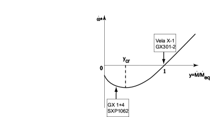
Figure 3: An illustration of the dependence of $\dot{\omega}^{*}$ on the dimensionless accretion rate $y$. In fact as $y\to 0$, $\dot{\omega}^{*}$ approaches some negative value since the neutron star enters the propeller regime at small accretion rates. The figure shows the position in the diagram for equilibrium pulsars with $y\sim 1$ and for non-equilibrium pulsars at steady spin-down with $y<y_{cr}$

For a characteristic value of the accretion rate $\dot{M}_{16}\equiv\dot{M}/10^{16}$ g/s, the coefficients (not dependent on the accretion rate) will be equal to (in CGS units):

$$A\approx 7.46\times 10^{31}\tilde{K}K_{1}K_{3}\zeta^{-\frac{7}{11}}\mu_{30}^{\frac{1}{11}}\left(\frac{v_{8}}{\sqrt{\delta}}\right)^{-4}\left(\frac{P_{b}}{10\hbox{d}}\right)^{-1}$$ (41)

$$B\approx 6.98\times 10^{32}(1-z/Z)\tilde{K}K_{1}K_{3}\zeta^{-3/11}\mu_{30}^{{13}/{11}}\left(\frac{P^{*}}{100\hbox{s}}\right)^{-1}$$ (42)

The dimensionless factor $\delta<1$ takes into account the actual location of the gravitational capture radius.

4 Equilibrium pulsars

Figure 4: Torque-luminosity correlation in GX 301-2, $\dot{\omega}^{*}$ as a function of BATSE data (20-40 keV pulsed flux) near the equilibrium frequency Dor10 . The assumed X-ray flux at equilibrium (in terms of the dimensionless parameter $y$) is also shown by the vertical dotted line.

Figure 5: The same as in Fig. 5 for Vela X-1 (V.Doroshenko, PhD Thesis, 2010, IAAT)

For equilibrium pulsars we set $\dot{\omega}^{*}=0$ and from Equation (38) we get

$$Z_{eq}(\omega_{m}-\omega^{*})+z\omega^{*}=0\,.$$ (43)

Close to equilibrium we may vary (38) with respect to $\dot{M}$. It is convenient to introduce the dimensionless parameter $y\equiv\dot{M}/\dot{M}_{eq}$, so that close to equilibrium $y=1$. Clearly, $\dot{M}_{eq}$ represents the accretion rate at which $\dot{\omega}^{*}=0$:

$$\dot{M}_{eq}=\left(\frac{B}{A}\right)^{11/4}\,.$$ (44)

Close to equilibrium we may vary (38) with respect to $\dot{M}$. Variations in $\delta\dot{M}$ may in general be caused by changes in density $\delta\rho$ as well as in velocity of the stellar wind $\delta v$ (and thus the Bondi radius). For density variations only we find

$$Z_{eq,\rho}=\frac{I\frac{\partial\dot{\omega}^{*}}{\partial\dot{M}}|_{eq}}{\frac{4}{11}\omega^{*}R_{A}^{2}}\approx\ 2.52\left(\frac{\frac{\partial\dot{\omega}^{*}}{\partial y}|_{y=1}}{10^{-12}}\right)\left(\frac{P^{*}}{100s}\right)\zeta^{-4/11}\dot{M}_{16}^{-7/11}\mu_{30}^{-12/11}\,.$$ (45)

The equilibrium period of an X-ray pulsar with known NS magnetic field is:

$$P_{eq}\approx 940[\hbox{s}](1-z/Z_{eq})\zeta^{4/11}\mu_{30,eq}^{12/11}\left(\frac{P_{b}}{10\hbox{d}}\right)\dot{M}_{16}^{-4/11}\left(\frac{v_{8}}{\sqrt{\delta}}\right)^{4}\,.$$ (46)

Because of the strong dependence of the equilibrium period on wind velocity, for pulsars with independently known magnetic fields $\mu$ it is more convenient to estimate the wind velocity, assuming $P*=P^{*}_{eq}$:

$$\frac{v_{8}}{\sqrt{\delta}}\approx 0.57(1-z/Z_{eq})^{-1/4}\zeta^{-1/11}\dot{M}_{16}^{1/11}\mu_{30,eq}^{-3/11}\left(\frac{P_{*}/100\hbox{s}}{P_{b}/10\hbox{d}}\right)^{1/4}\,.$$ (47)

If $(\partial\dot{\omega}/\partial y)_{eq}$ is also measured, then equating $Z_{eq}$ to the rhs of (37) we find the value of the magnetic moment of the neutron star only from the pulsar equilibrium period and the derivative $(\partial\dot{\omega}/\partial y)_{eq}$:

$$\mu_{30,eq}^{13/11}\approx 3.9\left(\frac{\frac{\partial\dot{\omega}^{*}}{\partial y}|_{y=1}}{10^{-12}\hbox{rad/s}^{2}}\right)\left(\frac{P^{*}}{100s}\right)(\tilde{K}K_{1}K_{3})^{-1}\zeta^{3/11}\dot{M}_{16}^{-3/11}\,.$$ (48)

If $\mu$ is independently measured, (48) allows us to determine the dimensionless complex of coefficients of the theory $\tilde{K}K_{1}K_{3}\zeta^{-3/11}$:

$$\tilde{K}K_{1}K_{3}\zeta^{-3/11}\approx 3.9\left(\frac{\frac{\partial\dot{\omega}^{*}}{\partial y}|_{y=1}}{10^{-12}\hbox{rad/s}^{2}}\right)\left(\frac{P^{*}}{100s}\right)\dot{M}_{16}^{-3/11}\mu_{30}^{-13/11}\,.$$ (49)

Table 1: Parameters for the equilibrium X-ray pulsars.

$$\begin{array}[]{lcc}\hline\cr\hbox{Pulsar }&\lx@intercol\hfil\hbox{Equilibrium pulsars }\hfil\lx@intercol\\ \hline\cr&{\rm GX301-2}&{\rm VelaX-1}\\ \hline\cr\lx@intercol\hfil\hbox{Measured parameters}\hfil\lx@intercol\\ \hline\cr P^{*}{\hbox{(s)}}&680&283\\ P_{B}{\hbox{(d)}}&41.5&8.96\\ v_{w}{\hbox{(km/s)}}&300&700\\ \mu_{30}&2.7&1.2\\ \dot{M}_{16}&3&3\\ \frac{\partial\dot{\omega}}{\partial y}\arrowvert_{y=1}{\hbox{(rad/s}^{2})}&1.5\cdot 10^{-12}&1.2\cdot 10^{-12}\\ \hline\cr\lx@intercol\hfil\hbox{Derived parameters}\hfil\lx@intercol\\ \hline\cr f(u)\zeta^{-7/11}&0.30&0.32\\ \tilde{K}K_{1}K_{3}\zeta^{-3/11}&9.1&7.9\\ \frac{v_{w,min}}{\sqrt{\delta}}(1-z/Z)^{1/4}\zeta^{1/11}\hbox{(km/s)}&540&800\\ \hline\cr\end{array}$$

Let us apply (49) to two equilibrimu X-ray pulsars in which all four observable quantities ($\mu$, $\dot{M}$, $P^{*}$, and $\partial\omega^{*}/\partial\dot{M}$) are known: GX 301-2 and Vela X-1 (see Table 1). The main result is that the dimensional complex $\tilde{K}K_{1}K_{3}\zeta^{-3/11}\sim 10$ in both cases. As factors $\tilde{K}$, $K_{1}$ and $\zeta^{-3/11}$ are of the order of one, this suggests that $K_{3}\sim 10$. Therefore, the size of the bottom part of the boundary layer with linear angular velocity dependence on radius, where most of the angular momentum is transferred from the magnetosphere to the shell, $\zeta^{\prime}R_{A}\sim 0.1R_{A}$ in both cases.

At $y_{cr}=(3/7)^{11/4}\approx 0.097$ the dependence $\dot{\omega}^{*}(y)$ reaches minimum (see Fig. 3). Apparently, depending on whether $y>y_{cr}$ or $y<y_{cr}$, correlated changes of $\delta\dot{\omega}^{*}$ with X-ray flux should have different signs (see Fig. 3). Indeed, for GX 1+4 in 1997ApJ…481L.101C and 2012A&A…537A..66G a positive correlation of the observed $\delta\dot{P}^{*}$ with $\delta\dot{M}$ was found using the CGRO BATSE and Fermi GBM data. This means that there is a negative correlation between $\delta\dot{\omega}^{*}$ and $\delta\dot{M}$, suggesting $y<y_{cr}$ in this source.

The application of the elaborated theory of subsonic wind accretion to non-equilibrium pulsars is discussed in 2012MNRAS.420..216S , 2013arXiv1302.0500S and elsewhere in this volume KPmagbound .

Acknowledgements. The authors acknowledge the Organizers of this Workshop and RFBR grant 12-02-00186a for support.

References

- (1) B.A. Fryxell, R.E. Taam, ApJ 335, 862 (1988)
- (2) M. Ruffert, A&A 346, 861 (1999), arXiv:astro-ph/9903304
- (3) T. Nagae, K. Oka, T. Matsuda, H. Fujiwara, I. Hachisu, H.M.J. Boffin, A&A 419, 335 (2004), arXiv:astro-ph/0403329
- (4) J. Arons, S.M. Lea, ApJ 207, 914 (1976)
- (5) A.F. Illarionov, R.A. Sunyaev, A&A 39, 185 (1975)
- (6) N. Shakura, K. Postnov, A. Kochetkova, L. Hjalmarsdotter, MNRAS 420, 216 (2012), 1110.3701
- (7) R.F. Elsner, F.K. Lamb, ApJ 215, 897 (1977)
- (8) A.S. Kompaneets, Zh. Eksp. Theor. Phys. 31, 876 (1956)
- (9) R. Weymann, Physics of Fluids 8, 2112 (1965)
- (10) D.J. Burnard, J. Arons, S.M. Lea, ApJ 266, 175 (1983)
- (11) N.I. Shakura, K.A. Postnov, A.Y. Kochetkova, L. Hjalmarsdotter, Physics-Uspekhi 56, 321 (2013), 1302.0500
- (12) R.V.E. Lovelace, M.M. Romanova, G.S. Bisnovatyi-Kogan, MNRAS 275, 244 (1995), arXiv:astro-ph/9412030
- (13) L.G. Loitsyanskii, Mechanics of Liquids and Gases, Pergamon Press Oxford (1966)
- (14) V. Doroshenko, A. Santangelo, V. Suleimanov, I. Kreykenbohm, R. Staubert, C. Ferrigno, D. Klochkov, A&A 515, A10 (2010)
- (15) D. Chakrabarty, L. Bildsten, M.H. Finger, J.M. Grunsfeld, D.T. Koh, R.W. Nelson, T.A. Prince, B.A. Vaughan, R.B. Wilson, ApJ 481, L101 (1997), arXiv:astro-ph/9703047
- (16) A. González-Galán, E. Kuulkers, P. Kretschmar, S. Larsson, K. Postnov, A. Kochetkova, M.H. Finger, A&A 537, A66 (2012), 1111.6791
- (17) K.A. Postnov, N.I. Shakura, A.Y. Kochetkova, L. Hjalmarsdotter, this volume (2013)