A comparative study of radio halo occurrence in SZ and X-ray selected galaxy cluster samples

Abstract

We aim at an unbiased census of the radio halo population in galaxy clusters and test whether current low number counts of radio halos have arisen from selection biases. We construct near-complete samples based on X-ray and Sunyaev-Zel’dovich (SZ) effect cluster catalogs and search for diffuse, extended (Mpc-scale) emission near the cluster centers by analyzing data from the NRAO Very Large Array Sky Survey. We remove compact sources using a matched filtering algorithm and model the diffuse emission using two independent methods. The relation between radio halo power at 1.4 GHz and mass observables is modeled using a power law, allowing for a ‘drop-out’ population of clusters hosting no radio halo emission. An extensive suite of simulations is used to check for biases in our methods. Our findings suggest that the fraction of targets hosting radio halos may have to be revised upward for clusters selected using the Sunyaev-Zel’dovich effect: while approximately 60% of the X-ray selected targets are found to contain no extended radio emission, in agreement with previous findings, the corresponding fraction in the SZ selected samples is roughly 20%. We propose a simple explanation for this selection difference based on the distinct time evolution of the SZ and X-ray observables during cluster mergers, and a bias towards relaxed, cool-core clusters in the X-ray selection.

1 Introduction

Clusters of galaxies are the relatively recent descendants of rare high-density fluctuations in the early universe. The extensive use in cosmology of this high-mass end of gravitationally collapsed objects relies largely on our understanding of the properties of the intra-cluster medium (ICM). The ICM is predominantly a fully ionized primordial plasma containing about 90% of the cluster baryonic mass, and reaching very high temperatures ($T\sim 2-10$ keV) as it gathers in the deep cluster potential well. There are two basic ways of detecting the ICM: direct detection through the thermal bremsstrahlung in the X-ray regime, and detection of the spectral distortion of the cosmic microwave background radiation (CMB) in the millimeter regime due to inverse Compton scattering. The latter is the Sunyaev-Zel’dovich (SZ) effect (Sunyaev & Zeldovich, 1972, 1980).

While surveys of galaxy clusters are concerned with the dominant thermal component of the ICM, the plasma is also host to a population of ultra-relativistic particles, i.e. cosmic rays. Prominent evidence for a non-thermal population, as well as cluster-wide magnetic fields, comes from the observation of diffuse synchrotron emission in some galaxy clusters. These extended radio sources have a typical size of $\sim 1$ Mpc, and are not associated with any individual galaxies. They are broadly split into radio halos and radio relics depending on their central or peripheral position in the clusters, as well as on geometry and extent of polarization. While both radio relics and radio halos are thought to be associated with cluster merger processes, radio halos are of particular interest due to their similarity in spatial distribution with the thermal ICM (e.g. Govoni et al., 2001) and their scaling with cluster mass as measured by the $L_{\mathrm{X}}-P_{\mathrm{radio}}$ correlation (e.g. Liang et al., 2000; Brunetti et al., 2009). As such, they are an important instrument in understanding the physics of cluster mergers, and can possibly even trace the redshift evolution of the cluster merger fraction.

The current understanding is that radio halos are relatively rare, with only a few tens of objects unambiguously detected to date (Feretti et al., 2012). Such low numbers stand in stark contrast to the number of X-ray or SZ selected clusters in various all sky surveys. The rarity of radio halos in turn prohibits their use in the statistical studies of large scale structure formation. However, a possible source of bias is that almost all the current radio halo data comes from follow-up observation of previously known X-ray clusters, either from ad-hoc collections (Giovannini et al., 2009; van Weeren et al., 2011b) or using X-ray flux limited samples (Venturi et al., 2008; Rudnick & Lemmerman, 2009; Kale et al., 2013). Therefore, the small number of radio halos can, in part, be the result of a selection bias that takes effect while correlating one indicator of the thermal ICM (its total X-ray luminosity) with one indicating its non-thermal energy. Recent discoveries of radio halos in a few clusters with very low X-ray luminosities (Giovannini et al., 2011), as well as the lack of a prominent radio halo in some X-ray luminous mergers (e.g. A2146: Russell et al., 2011) indeed raise questions of a possible selection bias regarding radio halo observations in X-ray selected clusters.

Predictions for radio halo counts in galaxy clusters also remain highly uncertain, lacking a proper understanding of their origin. The observed synchrotron emission requires acceleration of charged particles, and there are currently two different frameworks for mechanisms that can produce relativistic particles consistent with the radio emission observed at GHz-frequencies. ‘Primary’ (or turbulent re-acceleration) models assume that a seed population of high-energy electrons is re-accelerated through turbulence by the second order Fermi process (Schlickeiser, Sievers & Thiemann, 1987; Petrosian, 2001; Brunetti et al., 2001), while ‘secondary’ (or hadronic) models rely on the continuous injection of relativistic electrons by hadronic collisions between thermal and cosmic ray protons (e.g. Dennison, 1980; Blasi & Colafrancesco, 1999). The rarity of radio halos and a strong bi-modality of clusters in the radio/X-ray correlation indeed suggest a preference towards the primary (turbulent) re-acceleration models. Since the high energy protons are long-lived, radio halos powered by electrons originating from their collisional decay should be less sensitive to the cluster dynamical state (but see Enßlin et al. (2011) for alterations in the basic hadronic model to explain bi-modality). The separation of these two models is somewhat historic, but it is unlikely that both play a dominant role in powering radio halos. Predictions based on turbulent re-acceleration models contain a large number of free parameters that are matched to observations, and consequently the expected radio halo count in the sky based on these models has considerable uncertainties (Cassano et al., 2010). In light of the powerful all-sky radio surveys that are being prepared (e.g. LOFAR, ASKAP, MeerKAT) or will become operational in the coming decade (SKA), it is urgent to quantify the radio halo fraction in clusters in an unbiased manner.

In a previous work, we presented the first radio-SZ correlation results for radio halos with the aim of understanding possible selection biases and their true mass scaling (Basu, 2012, hereafter B12). In line with the expectation that radio halo power correlates with cluster mass, we found a clear correspondence between these two observables. More significantly, the strong bi-modal division present in the radio X-ray correlation appeared much reduced. However, we could neither quantify the selection bias nor determine the true rate of occurrence of radio halos in clusters in a given mass bin, since the B12 results were based on an ad-hoc selection of known radio halo clusters that were also present in the Planck ESZ catalog (Planck Collaboration, 2011a). The present work builds upon the early results presented in B12, and constitutes the first attempt to carry out an unbiased study of the radio halo population in an SZ selected cluster sample.

We analyze archived data from the VLA NVSS survey (Condon et al., 1998) to measure the extended radio emission in two samples of galaxy clusters and constrain the relation between mass and radio power. Data with higher sensitivity, better $uv$ coverage and greater resolution are available for many of our targets. However, to avoid biasing our results towards these systems, we refrain from using these data. We take great care to remove flux contributions from the peripheral radio relics as well as radio lobes and other extended emission from radio galaxies, although contamination from some radio relics and radio mini-halos cannot be ruled out. We carry out a two-component regression analysis to simultaneously model (i) the scaling of radio halo power with SZ and X-ray mass observables and (ii) the fraction of the cluster population hosting no radio halos. One of the main scientific results of the current paper is this radio halo “dropout fraction” found from uniformly selected X-ray and SZ cluster samples.

In Section 2 we discuss the selection of our samples. Section 3 is concerned with the analysis of the radio data, and the extraction of the extended radio component from the NVSS maps. We describe our mass-luminosity relation regression analysis in Section 4, and discuss systematic effects in Section 5. The results are presented in Section 6, along with comparisons with previous results, and in Section 7 we speculate on the cause for the measured selection difference in SZ and X-rays. We summarize our work and present our conclusions in Section 8. For all results derived in this work we assume a $\Lambda$CDM concordance cosmology with $h=0.7$, $\Omega_{m}h^{2}=0.13$ and $\Omega_{\Lambda}=0.74$.

2 Cluster samples

Our samples are extracted from the 2013 Planck catalog of Sunyaev-Zel’dovich sources (henceforth the PSZ sample, Planck Collaboration, 2013b) and a composite sample of X-ray selected clusters extracted from the REFLEX (Böhringer et al., 2004), NORAS (Böhringer et al., 2000), MACS (Ebeling, Edge & Henry, 2001), BCS (Ebeling et al., 1998) and eBCS (Ebeling et al., 2000) clusters catalogs (henceforth the X-ray, or simply X, sample).

The REFLEX sample covers the southern sky and is more than 90% complete above a flux limit of $3\times 10^{-12}\text{erg}~{}\text{s}^{-1}~{}\text{cm}^{-2}$ in the X-ray soft band (0.1$-$2.4 keV). The BCS sample comprises the 201 X-ray-brightest clusters of galaxies in the northern hemisphere with measured redshifts $z\leq 0.3$ and fluxes higher than $4.4\times 10^{-12}\text{erg}~{}\text{s}^{-1}~{}\text{cm}^{-2}$ (0.1$-$2.4 keV). eBCS is the low-flux extension of this sample, with a corresponding flux limit of $2.8\times 10^{-12}\text{erg}~{}\text{s}^{-1}~{}\text{cm}^{-2}$, and including some objects with $z>0.3$. Although the BCS$+$eBCS sample has 90% completeness, it does not cover the full northern hemisphere, and the completeness deteriorates quickly above $z>0.3$. For these reasons we also include the NORAS and MACS catalogs to arrive at a nearly complete sample within our selection as described below. For all X-ray cluster data, we use the MCXC meta-catalog of Piffaretti et al. (2011), referring to the original catalogs only for the uncertainties in the measured X-ray luminosities.

The selection of targets is based on considerations of (i) the recovery of extended structures with the VLA NVSS survey, (ii) the possible confusion of extended radio emission with radio galaxies, (iii) the sky coverage of the NVSS survey and (iv) completeness above a given mass threshold. The mass threshold is defined in terms of integrated Comptonization for the PSZ sample, and in terms of X-ray luminosity for the X-ray sample, as described below.

We consider only targets with redshifts exceeding $z=0.1$. At this redshift, the typical physical scale of a radio halo of one Mpc translates into an angular scale of $\sim 9^{\prime}$. Although the recovery of larger structures is in principle possible with the VLA, we must consider that the NVSS survey is made up of snapshot observations lacking in $uv$-coverage. As shown in section 6.2, the NVSS derived surface brightness of targets with confirmed radio halos approaching our thus imposed size limit (translating into an effective redshift limit) are statistically consistent with published results from more extensive observations, although results for individual targets show strong variations due to differences in the methods used for extracting the extended radio emission.

At a redshift of 0.4, one Mpc corresponds to roughly five times the NVSS beam full-width at half-maximum (FWHM). At even greater redshifts, it is conceivable that our algorithms for separating the extended emission from point sources (Section 3.1) can fail. In addition, at high redshifts the radio halo flux drops rapidly due to cosmological dimming and the K-correction (3.2.2), so the confusion with the other radio emitting sources in a cluster field becomes difficult to separate in the NVSS maps. For this reason, we impose an upper limit of $z=0.4$.

The NVSS covers the sky above declination $-40^{\circ}$. We restrict our samples to targets with $\delta>-39^{\circ}$ to avoid the edges of the NVSS survey.

As a mass measure we use $M_{500}$, the mass enclosed within the corresponding radius $r_{500}$ inside which the mean mass density is 500 times the critical density of the universe at the redshift of the target. In practice, a limiting mass translates into limiting values of integrated Comptonization for the PSZ sample and X-ray luminosity for the X-ray sample. In the following we discuss how masses are estimated in the two samples, and how these are used for selecting sub-samples for the radio halo analysis.

2.1 Mass estimates in the PSZ sample

The primary SZ observable in the PSZ sample is $Y_{500}$, the integrated Comptonization within $r_{500}$. We denote the intrinsic Comptonization as

$$Y_{\text{SZ}}=E(z)^{-2/3}D^{2}_{A}Y_{{500}},$$ (1)

where $D_{A}$ is the angular diameter distance and $E^{2}(z)=\Omega_{M}(1+z)^{3}+\Omega_{\Lambda}+\Omega_{k}(1+z)^{2}$ is the normalized expansion rate of the universe. The $E(z)^{-2/3}$ term is close to unity in the redshift range relevant for this work.

We estimate $M_{500}$ from the intrinsic Comptonization using the baseline relation of Planck Collaboration (2013a) according to

$$\left[\frac{Y_{\text{SZ}}}{10^{-4}~{}\text{Mpc}^{2}}\right]=10^{-0.19}\left[\frac{(1-b)~{}M_{500}}{6\times 10^{14}~{}M_{\odot}}\right]^{1.79},$$ (2)

where the factor $(1-b)$ accounts for bias due to the hydrostatic assumption. We use the best-fit value of 0.8 for this bias parameter.

Because of the large beam, $Y_{500}$ cannot be measured blindly with high accuracy from the Planck data. For this reason the PSZ catalog offers different estimates of $Y_{{500}}$ with different size priors from external validation (Planck Collaboration, 2013b). Because X-ray priors are not available for many clusters, we use the $Y_{z}$ estimates, which are based on breaking the size-flux degeneracy with the $M_{500}-Y_{\mathrm{SZ}}$ relation (see Planck Collaboration, 2013b, and references therein).

2.2 Mass estimates in the X-ray sample

For the X-ray sample we start with the $L_{X,500}-M_{500}^{\text{HE}}$ scaling of Arnaud et al. (2010), using the X-ray luminosities from the MCXC catalog (Piffaretti et al., 2011). As these masses are derived under the assumption of hydrostatic equilibrium, we correct them by the bias factor $(1-b)$ discussed in Section 2.1. For brevity, we will use the notation $L_{\mathrm{X}}$ in place of $L_{X,500}$ for the remainder of this work.

As noted by Planck Collaboration (2011b), $Y_{500}$ predicted by MCXC X-ray luminosities are somewhat low due to the fact that X-ray selection is more sensitive to the presence of cool-cores, and we expect this to translate into a difference in our two mass estimators. To test this, we directly compare the derived masses where they are available from both the MCXC and PSZ catalogs. The result, as expected, are slightly higher masses when using Eq. (2) for the same objects, with an average ratio of $1.24$. In order to allow similar mass cuts in both samples, we correct the MCXC masses by this factor. We emphasize that although our mass estimators may be biased, our main objective of having comparable mass estimates in both samples is thus guaranteed.

2.3 Mass selection

We consider two types of samples, using on the one hand a redshift-dependent mass cut, and on the other hand a constant mass cut. We discuss these in turn.

The redshift-dependent mass selection comes from the Planck SZ cluster sample used for cosmological analysis (Planck Collaboration, 2013a), and consists of 189 clusters of galaxies. Even though the SZ effect is expected to provide a redshift-independent mass selection in the ideal case, this does not account for instrumental effects. Due to the large effective beam area of Planck, the limiting mass at which a cluster can be reliably detected increases rapidly up to $z\sim 0.6$ and flattens thereafter. We use this COSMO sub-sample of PSZ clusters for our work, all but one of which have known redshifts. After applying our redshift and declination selection we arrive at a sample of 90 targets (henceforth the PSZ(V) sub-sample). Translating the completeness criterion of the Planck COSMO clusters to the X-ray sample is difficult because the PSZ completeness depends on the Galactic and point source masks and the varying noise properties across the sky, the latter being a by-product of the matched-filtering cluster detection algorithm. We therefore use the 50% mean completeness limit across the entire sky for our mass threshold, as described by Planck Collaboration (2013a), to define a sharp (redshift dependent) mass cut for the X-ray clusters. In conjunction with the redshift and declination cuts as above, this yields a sample of 86 targets (henceforth the X(V) sub-sample).

Having a redshift dependent mass selection is contrary to the common practice in previous radio halo studies, and also makes it more difficult to address the question of what fraction of clusters host a radio halo in a given mass bin. We therefore also consider a more conventional redshift-independent mass cut at a constant value of $M_{500}=8\times 10^{14}~{}M_{\odot}$. This yields 79 targets from PSZ and 78 targets from X-ray. We denote these sub-samples PSZ(C) and X(C), respectively. The X-ray luminosity corresponding to this constant mass cut is $4.6\times 10^{44}E(z)^{7/3}$ erg/s. In our concordance cosmology this translates into $5.2\times 10^{44}$ erg/s at $z=0.1$ and $7.7\times 10^{44}$ at $z=0.4$, comparable to previous radio halo studies in X-ray selected clusters (Venturi et al., 2008, e.g., used a constant $L_{\mathrm{X}}$ cut at $5.0\times 10^{44}$ erg/s in the redshift range $0.2<z\leq 0.4$).

We note that the constant-mass selected PSZ(C) sub-sample is artificially cut because many of the cluster candidates in the PSZ catalog lack redshifts. The high mass threshold applied in this work nonetheless guarantees a high degree of completeness, such that a true mass selected sample with comparable mass and redshift selection would not make a significant statistical difference.

As part of the analysis, we remove NVSS fields in which bright point sources and their side lobes cause our point source removal algorithm (Section 3.1) to fail (in the sense that it does not converge on a point source free map). The mass and redshift selections are summarized in Table 1 and Fig. 1. The redshift distribution of the selected sources are similar between the two main samples for each type of mass selection, as is illustrated in Fig. 2.

Table 1: Cluster samples. The primary selection is based on the redshift, declination, and the $Y_{\text{SZ}}$ (or $L_{\mathrm{X}}$) cut. Subsequent data quality control removes objects with strong interferometric noise artifacts around bright ($\ {\raise-2.15277pt\hbox{$\buildrel>\over{\sim}$}}\ 1$ Jy) anywhere in the field. The designators V and C indicate the redshift dependent and constant mass selections, respectively.

Sub-sample	Mass	Primary	Flagged due	Final
	limit	selection	to bad data	sample
PSZ(V)	$z$-dependent	90	1	89
X(V)	$z$-dependent	86	1	85
PSZ(C)	$8\times 10^{14}M_{\odot}$	79	0	79
X(C)	$8\times 10^{14}M_{\odot}$	78	1	77

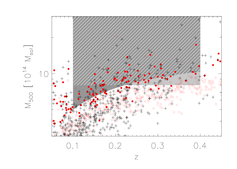
Figure 1: Mass and redshift selection. Circles represent the PSZ sample, with filled symbols indicating the PSZ cosmology sample. Plus signs represent the X-ray sample. Our two selection functions are indicated by the shaded regions: a constant mass threshold of $8\times 10^{14}M_{\odot}$ in light gray, and a redshift dependent mass threshold defined to mimic the PSZ cosmology sample selection in dark grey (see text). The hatched region marks the overlap between the two selections.

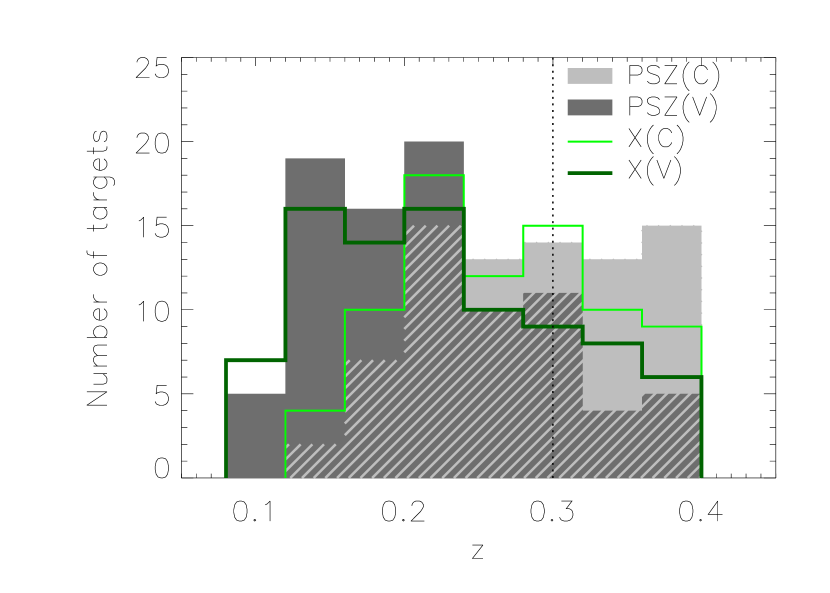
Figure 2: Redshift distribution in the two samples and using the two different mass selection criteria (the hatched region is the overlap of the PSZ(V) and PSZ(C) samples). The redshift distributions of the PSZ and X samples start to diverge slightly at approximately $z=0.3$, indicated by the vertical dotted line.

3 Analysis of the NVSS data

For each field in our two samples, we obtain a $1.3^{\circ}\times 1.3^{\circ}$ 1.4 GHz radio map from the NVSS archive. The NVSS synthesized beam has a FWHM of 45^′′, and the rms noise is about 0.45 mJy/beam. These numbers are approximately uniform across the entire survey area.

In Section 3.1 we describe the different filtering steps applied to the radio maps in order to separate the extended radio emission from other components such as background and foreground point sources and radio galaxies (typically brightest cluster galaxies, BCG). For simplicity, we refer to these contaminating sources simply as radio point sources, although in many cases they may not be point-like with respect to the NVSS beam. In Section 3.2 we discuss two independent methods of measuring the extended radio emission.

3.1 Filtering of the maps

Because point sources cover a wide dynamic range in flux density and considering the relatively poor resolution of NVSS, there is no single method that will reliably separate them from an extended component. We have considered and tested several methods of extracting the extended emission, and have found the direct removal of point sources to be the most robust. A matched filter applied directly to the extended emission is found to work poorly because the tails of compact sources are found to contaminate the extracted signal. In addition, the morphology of the sought radio emission is not known a priori.

The multi-scale spatial filter of Rudnick (2002) was used for similar analyses by, e.g., Rudnick & Lemmerman (2009) and Brown et al. (2011). This filtering method can cause a low-flux bias in case there are significant substructures on the diffuse emission, and can potentially suffer from contamination due to the tails of bright sources. As there is furthermore no clear definition of the recovered scale, we will not use this filtering method.

We follow three separate, consecutive steps for the removal of point sources. Regions around bright sources ($S_{1.4}\ {\raise-2.15277pt\hbox{$\buildrel>\over{\sim}$}}\ 20$ mJy) are completely cut from the map, weaker sources are fitted with Gaussians and subtracted from the map, and finally the residual map is low-pass filtered to remove point source emission below the detection threshold.

We identify point sources by a matched filtering algorithm. Because compact radio sources can be slightly resolved by the NVSS beam, we pre-smooth the NVSS map with a Gaussian in order to allow for a better matching of sources to a point source template. The level of smoothing is based on the maximum size of a radio galaxy belonging to the cluster, which we assume to be 100 kpc. The angular equivalent of this extent at the redshift of the cluster, $\Theta_{100\,\text{kpc}}$, is used as the FWHM of a Gaussian with which we smooth the map. The final resolution of the map is thus

$$\Theta_{S}=\sqrt{\Theta_{100\,\text{kpc}}^{2}+\Theta_{\text{NVSS}}^{2}},$$ (3)

where $\Theta_{\text{NVSS}}$ is the 45^′′ FWHM of the NVSS beam. The intrinsic NVSS resolution is effectively degraded by 8% at $z=0.4$ and by roughly 60% at $z=0.1$. We construct a template source with FWHM $\Theta_{S}$ as input for the matched filter. In order to avoid contamination from the extended radio emission, we taper scales larger than three times the NVSS beam FWHM in the matched filtering.

The matched filtering algorithm is iterative in the sense that we re-estimate the noise power spectrum in the 1.4 GHz radio map after removing each point source, starting with the brightest one, in order to successively increase the accuracy of the filter. Assuming that there are no preferred directions in the map, the noise power spectrum is radially averaged.

The peak of the brightest radio source in the filtered map can be offset for two reasons: the radio source can be extended with respect to the map resolution, and the noise power spectrum can be overestimated. In fact, in most cases both effects are strong enough to affect the result. Thus, in each iteration we fit an elliptical Gaussian model to the radio source in the original unfiltered map. For the modeling we constrain the centroid position to be within $\frac{1}{5}$ of the extent of the NVSS beam FWHM. We also constrain the intrinsic (deconvolved) source FWHM to be less than 100 kpc (major and minor axes).

Sources brighter than 20 mJy are found to leave residual structures after being subtracted, due to the NVSS beam not being a perfect Gaussian. When such a source is found by our algorithm, we flag a region around the source corresponding to a radius where the model flux has dropped below 0.1 mJy/beam, which is well below the rms level of the NVSS survey. For any source below 20 mJy, the model is subtracted from the map before a new noise power spectrum is estimated and the next iteration takes place.

In each iteration we also re-estimate the rms of the radio map, and stop iterating at a radio source peak signal-to-noise ratio of 3. At this significance level a relatively high number of spurious detections is expected; thus we take care to model both positive and negative peaks. Conversely, there will be a significant population of sources below our significance threshold, which can seriously affect the subsequent measurement of the extended component. For this reason we use a Butterworth filter to low-pass filter the residual map, effectively removing remaining structures smaller than 200 kpc in extent. Compared to $r_{500}$, this scale is very small (Fig. 3). Consequently, this low-pass filter will not affect the sought-after radio halo emission in a significant way, but will minimize the contamination from radio mini-halos which are comparable to the chosen filter size.

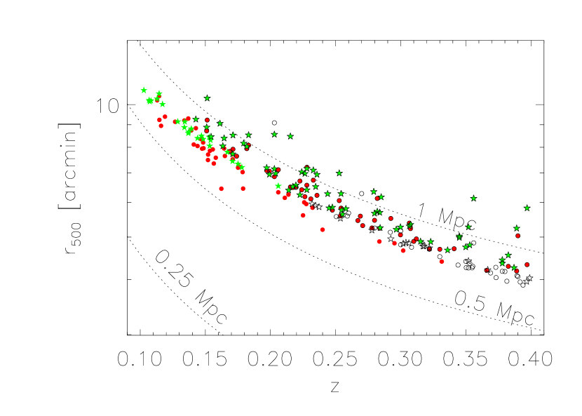
Figure 3: Physical scale $r_{500}$ vs. redshift for the PSZ (circles) and X-ray (stars) samples. Filled symbols indicate the redshift dependent (V) samples while open symbols represent the samples selected by constant mass (C). Dotted lines indicate constant physical scales.

3.2 Extraction of the extended signal

Measuring the luminosity of the extended radio emission component in any single galaxy cluster using the relatively shallow NVSS data is the central challenge of this work. We consider two methods here. First, we take the approach of fitting a model to each target. In most cases the signal-to-noise ratio of a single target will be too low to allow for a detailed modeling of the emission. For this reason, we make the simplifying assumption of self-similarity, allowing us to stack our samples to obtain a high-fidelity measurement of the mean radial profile. This approach is considered in Sections 3.2.1 and 3.2.2

Because the assumption of self-similarity may not be valid, we consider a second approach in which we integrate the flux in an appropriate aperture (we will use $0.5\times r_{500}$ for reasons explained below). This method is complicated by the fact that because we have blanked out several regions of most radio images, often including bright radio galaxies in the centers of galaxy clusters, there is missing information which in many cases cannot be reliably recovered. We consider the method in detail in Section 3.2.3.

3.2.1 Mean profile of the radio halo emission

In order to stack the maps, it is necessary to first scale them both to a common linear scale and to a common normalization to avoid over-weighting the radio-bright targets. We discuss each of these aspects in turn.

Scaling to a common linear scale is difficult because little is known about the expected physical extent of the radio emission. Cassano et al. (2007) constrained the linear sizes of radio halos by averaging their minimum and maximum extensions, and found a strong correlation of this size measure, $R_{H}$, with radio halo power $P_{1.4\,\text{GHz}}$. Although $R_{H}$ would seem a useful measure for the size of a radio halo we note that the scaling of $r_{500}$ and $R_{H}$ is non-linear, for which we cannot provide a feasible physical explanation. In this work, we scale the radio emission using $r_{500}$. This is a robust physical scale of clusters of galaxies and should also have a physical meaning for radio halos considering the strong correlation between radio halo power and SZ signal in a similar aperture shown in B12.

Scaling the normalization would ideally be done by dividing each map by the radio flux at some common physical radius. However, again due to the limited significance that we expect for most of our measurements, this is not possible. Instead we choose to scale each map by the total radio power. This poses the additional problem that the total radio power is not known until we have chosen the appropriate model to fit. It is thus necessary to proceed in an iterative way, where we first derive a radial profile (with the model described below) from a non-normalized stack (possibly biased towards radio-bright targets), then fit for total power, and finally derive a new profile from a stack where each map has been scaled according to the radio power thus found. We find that this approach converges very quickly, and that only two iterations are necessary.

In the first iteration, we assign equal weights to all fields, since the NVSS survey has very close to uniform rms. We then re-scale all radio images to $r_{500}$, adjusting the weights accordingly, before stacking the images and constructing the mean radial profile.

While we find that a number of models fit the resulting profiles, simple models with only one ‘shape’ parameter (such as a Gaussian) are insufficient. For reasons of convenience, we perform a fit using the functional form of the isothermal $\beta$-model:

$$S=S_{0}\left(1+\left(\frac{x}{x_{s}}\right)^{2}\right)^{(1-3\beta)/2}.$$ (4)

Here $S_{0}$ is an arbitrary normalization of the amplitude, and $x\equiv r/r_{500}$. The shape of the profile is determined by the parameters $x_{s}$, the scale radius in units of $r_{500}$, and $\beta$, which relates to the outer profile slope. Note that we use the $\beta$-model simply as a flexible parametric model to fit the extended emission $-$ there is no attempt at establishing a formal connection between the radio halo and the cluster SZ profile.

The fit is performed inside $0.5\times r_{500}$, corresponding to a median angular radius of $\sim 2.8^{\prime}$ in the PSZ sample, and a similar radius in the X-ray sample. We restrict the fit inside $0.5\times r_{500}$ for two reasons: (i) we want to minimize the contamination from extended radio relics that are typically found in the cluster outskirts, and (ii) there can be some attenuation of the radio emission in the outskirts due to the limited $uv$ coverage in the NVSS maps.

We carry out the radial fits separately for each sample, and find consistent results from the X-ray and PSZ samples. Combining in quadrature, we use the derived parameters to obtain total radio power measurements as discussed in Section 3.2.2, and use the results to re-normalize our maps for a new stacked profile, the result of which is shown for the PSZ sample in Fig. 4.

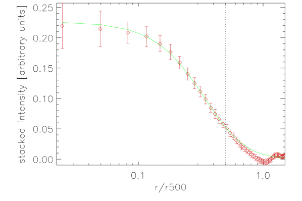
Figure 4: Stacked radial profile of radio emission normalized to $r_{500}$ and total radio power for the PSZ sample. The best-fit model is indicated by the solid curve. Only data within $0.5\times r_{500}$ (dashed line) is used for the fit.

The results of the second fit are presented in Table 2. We verify that an additional iteration produces results consistent with these. As the results from the two samples are consistent within uncertainties, we combine them to obtain a ‘universal’ profile, scaled at $r_{500}$. We use this profile to constrain the radio luminosity of each target as described next in section 3.2.2.

Table 2: Stacked radial fit results

Sample	$x_{s}$ ($r_{500}$)	$\beta$
PSZ	0.479 $\pm$ 0.105	1.673 $\pm$ 0.416
X-ray	0.468 $\pm$ 0.062	1.850 $\pm$ 0.285
combined	0.471 $\pm$ 0.048	1.793 $\pm$ 0.235

To investigate whether there is a mass dependence in the radio surface brightness profile, we also divide each sample into two bins, dividing at the median Comptonization of the PSZ sample and the corresponding X-ray luminosity. Within uncertainties we find no evidence of a mass dependence in the best-fit profile, and thus proceed with a common radial profile for all objects.

3.2.2 Radio measurements by radial fitting

In each cluster field, we use the radial model derived in the previous subsection, with the parameters $x_{s}$ and $\beta$ fixed to their combined best-fit values (bottom row of Table 2), to fit for the peak amplitude of the radio emission. Integrating over the resulting model out to $0.5\times r_{500}$, we derive the total radio power (within $r<0.5\times r_{500}$) from the flux $S_{\mathrm{1.4\,GHz}}$ according to

$$P_{\mathrm{1.4\,GHz}}\ =\ (4\pi\ D_{L}^{2})\ S_{\mathrm{1.4\,GHz}}\ \frac{{\cal K}(z)}{(1+z)},$$ (5)

where $S_{\mathrm{1.4\,GHz}}$ is the integrated flux density, $D_{L}$ is the cosmological luminosity distance and ${\cal K}(z)$ is the K-correction, accounting for the fact that due to the redshift, the observed flux corresponds to a rest frequency higher than 1.4 GHz. To compute the K-correction term, we assume that the radio flux scales with frequency as $S_{\nu}\propto\nu^{-1.2}$. Feretti et al. (2012) report spectral slope measurements over tens of radio halos, where the median is consistent with our assumed slope.

Integrating the radial profile only to half of $r_{500}$ implies that a significant fraction of the total radio flux is unaccounted for. Assuming the radial profile derived in Section  3.2.1, we account for this loss. Integrating the profile over the azimuthal angle and in radius out to $0.5\times r_{500}$ and to $r_{500}$ results in an effective correction factor of 1.46. Applying this correction, our quoted radio measurements are scaled to the region within $r_{500}$. We rely on our model rather than the data for this extrapolation because NVSS maps may not be sensitive to the largest scales (indeed some maps show negative artifacts at large radii), while quoting values only within $0.5\times r_{500}$ will cause a systematic under-estimation of the total radio halo fluxes when comparing with published results (see Section 5.6). The results of our work do not depend on this extrapolation.

The dominant source of statistical uncertainty in $P_{\mathrm{1.4~{}GHz}}$ is the residual noise due to unfiltered point sources and other compact objects in the map. We estimate this uncertainty in the flux measurement by inserting each fitted profile into 100 noise realizations based on the noise power spectrum of the filtered radio image and re-performing the fit. In order for the data to carry the same weight, we mask out the same regions in each mock image as were masked in the real radio map due to contamination by bright sources (see Section 3.1). We verify that the mean flux found by this method is consistent with the nominal flux in the map, and use the standard deviation of the integrated flux from the 100 realizations as an estimate of the uncertainty in our radio flux.

3.2.3 Radio measurements by direct integration

To verify that our flux extraction method is robust, we perform a separate analysis based on extracting the diffuse radio flux by direct integration in the map rather than by fitting a model. Even though the radial fitting method takes into account a variation in radio halo sizes scaled to the cluster mass, actual scaling of radio halo radii can be different, affecting our flux measurements.

The method of direct summation of flux inside the core region of clusters is somewhat complicated by the fact that the processed NVSS maps may have “holes” at the positions of bright point sources (Section 3.1). We fill in the holes by interpolating from the unmasked pixels at the edges, using the inverse distance squared between the pixels as the weight function. We note that this process will tend to underestimate the flux in cases where the peak of the diffuse radio emission coincides with a strong point source; however, simulations with radio emission constructed from the profile found in the previous subsection and with bright point sources added in the center indicate that the bias is at a level of 5% for the high redshift clusters, and much less at the median redshifts of our samples. We measure the extended radio flux in each NVSS map by summing the flux in an aperture, again corresponding to $0.5\times r_{500}$, and proceed to compute the luminosity as described in the previous subsection.

4 Regression analysis

In this section we outline our procedure for finding the best-fit empirical relation between radio power and the mass observable ($Y_{\text{SZ}}$ in the case of the PSZ sample and $L_{\mathrm{X}}$ in the case of the X-ray sample). We model the dependence using a power law, and perform the regression taking into account uncertainties in both coordinates, intrinsic scatter and what we call a dropout fraction term, quantifying the fraction of data points consistent with not belonging to the main distribution.

Regression of scaling relations is traditionally carried out in log-log space, where the problem of fitting a power law reduces to a linear regression problem. Even when errors are not log-normally distributed (which is rarely the case), this method can provide a good approximation of the assumed underlying power law, provided that measurement uncertainties are small. However, due to our data having relatively large uncertainties, particularly in the total radio power, and the measurements following close to normal distributions, we fit the scaling relations to the measurements directly in linear space. This also has the advantage that no special provisions are needed for non-detections; we can use all measured values (also negative ones) along with their uncertainties in a uniform way.

We fit the data to a power law relation of the form

$$y=f(x)=Ax^{B},$$ (6)

where, in our case, $y$ is the total radio power, and $x$ is the mass observable. We include in our analysis a fractional intrinsic scatter $\sigma_{\mathrm{F}}$ in radio power, such that the linear scatter at a given power is equal to $y\sigma_{\mathrm{F}}$. Note that just as fitting in log-log space implies log-normal scatter when using a $\chi^{2}$ formalism, fitting in linear space likewise implies some form of linear scatter (since scatter and uncertainties are on a equal footing in this formalism). Although this has the unfortunate disadvantage of allowing the $y$ variable to scatter below zero, which is unphysical, we find that a fractional scatter provides the best fit to our data.

There is a plethora of $\chi^{2}$-based methods described in the literature for finding the best-fit model when uncertainties are present both the dependent and independent variables. Here we follow a maximum-likelihood approach similar to that described by Kelly (2007), and we refer to that work for a detailed discussion. It is assumed that the independent variable is drawn from a distribution which is approximated by a mixture of $K$ Gaussians with normalization $\pi_{k}$, mean $\mu_{k}$ and variance $\tau^{2}_{k}$. Denoting the measured data as $\mathbf{z}=(\mathbf{y},\mathbf{x})$, the measured data likelihood function for data point $i$ is then a mixture of normal distributions with weights $\pi_{k}$, means $\zeta_{k}=(f(\mu_{k}),\mu_{k})$ and covariance matrices $\mathbf{V}_{k,i}$. The likelihood function is given by the product of the individual likelihoods of the data points,

$${\cal L}=\prod_{i=1}^{n}\sum_{k=1}^{K}\frac{\pi_{k}}{2\pi|\mathbf{V}_{k,i}|^{1/2}}\times e^{-\frac{1}{2}(z_{i}-\zeta_{k})^{\mathrm{T}}\mathbf{V}^{-1}_{k,i}(z_{i}-\zeta_{k})}.$$ (7)

We again refer to Kelly (2007, their section 4.1) for a detailed discussion on how the distribution of the independent variable is realized in practice. The covariance matrix of the $i$th data point and the $k$th Gaussian is given by

$$\textbf{V}_{k,i}=\left(\begin{array}[]{cc}\beta_{i}^{2}\tau_{k}^{2}+\sigma^{2}+\sigma^{2}_{y,i}&\beta_{i}\tau_{k}^{2}+\sigma_{xy,i}\\ \beta_{i}\tau_{k}^{2}+\sigma_{xy,i}&\tau_{k}^{2}+\sigma^{2}_{x,i}\end{array}\right),$$ (8)

where in our case $\sigma=y\sigma_{\mathrm{F}}$ and $\beta_{i}=\frac{\partial f}{\partial x}|_{x_{i}}$. The covariances $\sigma_{xy,i}$ are all assumed to be zero, while the variances $\sigma^{2}_{x,i}$ and $\sigma^{2}_{y,i}$ are derived from the individual measurement uncertainties on the mass estimators and radio halo powers, respectively.

There are several ways to accommodate the possibility of a bi-modality in $f(x)$. The most simple method would be to carry out the analysis excluding any data points that by some selection criterion are deemed to be consistent with zero radio luminosity. This can be accomplished, for example, by rejecting all data points below some significance threshold. However, such an algorithm is likely to introduce a bias in the estimated parameters because data points at the low $x$ end are also expected to have less radio emission.

A more robust estimate can be achieved by introducing a measure of bi-modality in the likelihood computation. To this end, we introduce a set of $N$ binary parameters $q_{i}$ in the likelihood, each of which is unity if the corresponding data point belongs to the “on-population” (the sought power law) and zero if the corresponding data point belongs to the “off-population” (no extended radio emission). The individual likelihood of data point $i$ needs to be modified in the case that $q_{i}=0$, in the sense that $\zeta^{\mathrm{off}}_{k}=(0,\mu_{k})$ and the covariance matrix $\textbf{V}_{k,i}$ reduces to the simple form

$$\textbf{V}^{\mathrm{off}}_{k,i}=\left(\begin{array}[]{cc}\sigma^{2}_{y,i}&\sigma_{xy,i}\\ \sigma_{xy,i}&\tau_{k}^{2}+\sigma^{2}_{x,i}\end{array}\right)$$ (9)

under the (rather straightforward) assumption that the off-population has zero mean and no intrinsic scatter. Including the new-found parameters in our analysis, we can still use Equation 7 to compute the likelihood.

The inclusion of the $q_{i}$ implies that we now have more parameters than data, this is not generally a reason for panic, in particular because each $q_{i}$ can only take on two discrete values. More importantly, however, we can marginalize over the nuisance parameters $q_{i}$ by replacing them with a single continuous variable, the dropout fraction, $g$, signifying the fraction of off-population measurements (see, e.g., Hogg, Bovy & Lang, 2010, for a similar argument). The likelihood for an individual data point then becomes

$$\begin{split}{\cal L}_{k,i}=&\frac{(1-g)\,\pi_{k}}{2\pi|\mathbf{V}_{k,i}|^{1/2}}e^{-\frac{1}{2}(z_{i}-\zeta_{k})^{\mathrm{T}}\mathbf{V}^{-1}_{k,i}(z_{i}-\zeta_{k})}\\ &+\frac{g\,\pi_{k}}{2\pi|\mathbf{V}^{\mathrm{off}}_{k,i}|^{1/2}}e^{-\frac{1}{2}(z_{i}-\zeta_{k}^{\mathrm{off}})^{\mathrm{T}}(\mathbf{V}^{\mathrm{off}}_{k,i})^{-1}(z_{i}-\zeta_{k}^{\mathrm{off}})}.\end{split}$$ (10)

This so-called mixture model is used for the remainder of this work.

We use a Bayesian method to estimate the best-fit parameters of the power law through a Markov Chain Monte Carlo (MCMC) approach. We run four parallel chains starting from dispersed initial values to check for convergence by correlating the resulting posterior distributions. The $68\%$ confidence interval is computed by integrating down from the maximum likelihood peak. We note that the dropout fraction and the intrinsic scatter have sharp boundaries at zero, imposed by physically motivated priors.

5 Control of systematics

Our final result will be the product of a rather complex analysis, involving filtering and flagging of the raw NVSS images as well as a non-standard method for estimating the power law relating the mass observable to radio power under the assumption of bi-modality. In this section we describe a series of simulations aimed at taking into account effects of radio point sources below the detection threshold, the flux extraction methods, and the fitting procedure. We rule out the possibility of bias due to radio lobes, and perform several null tests to check for residual source contamination or “clean bias” in the NVSS maps. In addition, we compare individual radio halo measurements to published results where available.

5.1 Model fitting

To test the model fitting analysis, we perform a Monte-Carlo simulation taking the best-fit parameter values from each sample (as obtained from the regression analysis of our X-ray and SZ samples; see Section 6) as input, and verifying that the results of the regression analysis are consistent with these input parameters.

We use the measured values of the independent variable ($Y_{\text{SZ}}$ or $L_{\mathrm{X}}$) as a starting point, and derive theoretical values of the dependent variable (radio power) using our bi-modal distribution: For each data point we use the best-fit power law parameters (with probability $1-g$) or set the radio halo power to zero (with probability $g$). Random noise at the level of the actual measurements is added to both variables, as well as random scatter in the dependent variable. This procedure is repeated several thousand times, and in each iteration we derive the best-fit parameters from the simulated data points.

We also allow the dropout fraction $g$ to vary in our simulation to investigate whether it can be biased low by our fitting method. In general, we find this not to be the case, as illustrated in Fig. 5 for the PSZ sample. The X-ray sample yields similar results. We also find that the input parameters, including the scatter, can be recovered to an accuracy better than the statistical uncertainties (Fig. 5).

Figure 5: Recovery of model parameters (power law slope $B$, linear scatter $\sigma$ and dropout fraction $g$) as a function of the input dropout fraction $g_{\mathrm{in}}$ from a set of 3000 PSZ-like simulations. The dotted lines indicate the input parameter values, which were kept constant excepting the dropout fraction. Vertical error bars indicate the spread in fitted (maximum likelihood) parameter values, and horizontal error bars indicate bin widths. Subscripts ‘ML’ and ‘in’ indicate maximum likelihood and input values, respectively. The seemingly peculiar behavior at $g_{\mathrm{in}}=0.65$ is the result of a statistical fluctuation slightly in excess of one sigma.

We find a slight underestimate of the intrinsic scatter, at a level of up to 5% in the PSZ sample and up to 7% in the X-ray sample, in the range of $g$ consistent with the respective best fits. We note, however, that this bias is well below the level of the statistical uncertainties in this parameter.

5.2 Effects of Filtering

We now turn our attention to any possible bias arising from the filtering of the radio maps. To this end, we fabricate $10^{4}$ maps with simulated extended radio signals using the radial profiles derived in Section 3.2.1. We generate each radio model randomly with model parameters in the range $0.1<z<0.4$, $0.8~{}\text{Mpc}<r_{500}<1.5~{}\text{Mpc}$ and $0<\log_{10}(S[\text{mJy}])<2.3$, resulting in a distribution that is by no means meant to be realistic, but will serve our purpose of investigating the effects of filtering. We add each radial model to a randomly chosen patch from the NVSS survey to ensure realistic noise properties. We do not add a population of radio point sources at this point, but consider this problem separately in Section 5.3

After passing the simulated maps through our filtering apparatus, we consider the fraction of the input flux that is recovered after filtering and point source blanking. Using both the radial fit and direct integration methods, we find that the recovered flux is very close to 100% of the input flux, with no detectable dependence on the level of the input flux or the linear size of the emission.

5.3 Effects of a faint radio point source population

It is possible that a population of faint point sources below the detection limit can mimic a diffuse extended radio emission. Integrating the 1.4 GHz volume-averaged cluster luminosity function of Lin & Mohr (2004) for luminosities below that corresponding to the completeness limit of the NVSS survey at the median redshifts of our samples results in a total point source contribution of several mJy assuming typical values of $r_{500}$, which is similar to typical flux levels of detected radio emission at the low-mass end of our samples. We therefore carry out a simulation to investigate whether there is a residual population of faint point sources that can contaminate our signal after the filtering process.

We model the cluster radio point source population from the luminosity function and radial distribution of the AGN and star-forming (SF) galaxies. For the AGN population, we use the luminosity function and radial distribution of Sommer et al. (2011), who determined the volume averaged radio luminosity function at 1.4 GHz in cluster environments from an optical sample of clusters and groups, to populate simulated fields with sources. For the star-forming galaxies, we use the luminosity function of Lin & Mohr (2004), which was determined at lower redshifts than that of Sommer et al. and thus has leverage on this relatively fainter population. We consider luminosities down to a limit of $10^{19}$ W Hz^-1. Extrapolating the luminosity function below this limit does not lead to an appreciable increase in total luminosity. The radial distribution of star-forming galaxies is difficult to decouple from that of the AGN population. Here we differentiate the integrated counts given by Coppin et al. (2011) to arrive at a radial profile, to populate simulated fields with the distribution of star-forming galaxies given by the luminosity function.

In simulating cluster fields, we follow the same procedure as outlined in Section 5.2, the only difference being the inclusion of the cluster point source populations. We also generate three sets of reference maps, containing (i) only the extended signal, (ii) only the point sources, and (iii) neither of these components.

After filtering, we investigate whether the output maps contain more signal than the reference maps with no point sources. We find this indeed to be the case, although the effect is small: For a halo with $r_{500}=1~{}\text{Mpc}$, the residual power is on the order of $1\times 10^{23}$ W Hz^-1, corresponding to less than $1$ mJy at $z=0.25$.

We find that, on average, the residual power scales with volume, as expected from the construction of the point source populations from volume averaged luminosity functions. We also find that the contaminating power increasing with redshift. This is related to the adaptive smoothing scale described in Section 3.1, and can be intuitively understood as it being harder to separate point sources from extended emission at higher redshifts where the size of these two components become more similar, given a constant resolution.

We find that the contaminating power is well fit by a power law of the form

$$P_{\text{contamin}}=C~{}{r_{500}}^{3}~{}(1+z)^{\gamma},$$ (11)

where $C$ is a normalization which has a slight dependence on the flux extraction method used, and $\gamma=6.5\pm 0.5$. We verify that the same result is obtained regardless of whether the full simulation or the point source-only simulation is used.

Correcting for the excess power, we further verify that the resulting distribution of flux from a simulation is consistent with the input flux, corrected for the finite aperture of the flux extraction (Fig. 6).

While the correction that we apply is a mean value, given a mass and redshift, the actual power excess will vary. We account for the scatter in the actual radio point source luminosity function in clusters as an additional systematic uncertainty. We use the standard deviation of excess signal from the simulations described above and add this quantity in quadrature to the measurement uncertainty from the filtered map.

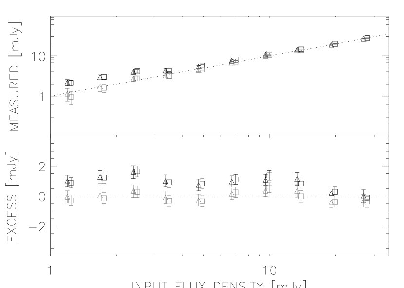
Figure 6: Measured (black) and bias corrected (gray) flux densities vs. input from simulations, using the radial fit (triangles) and direct integration (squares) methods of flux extraction. The measured values have been corrected for the finite aperture used (Section 5.2), while the bias corrected ones include an additional correction for residual flux from point sources (Section 5.3).

5.4 Radio lobes

We now consider whether extended radio lobes can contribute to the total derived extended radio luminosity. To this end, we extract cutouts from the VLA FIRST survey (Becker, White & Helfand, 1995) at the same frequency. The FIRST survey sky coverage is different from that of NVSS, and we find counterparts for about one-third of the target fields. For the latter, we visually inspect the FIRST maps, which have a resolution of 5^′′, and find radio lobes around bright sources within $r_{500}$ in more than half of the fields inspected. We find that virtually all radio lobes found in the FIRST maps are well within the regions that were flagged around bright NVSS sources due to our filtering algorithm (cf. Section 3.1), and thus conclude that unresolved radio lobes cannot contribute a significant fraction to our derived radio signals.

5.5 Null tests

In order to ascertain that there is no systematic contamination from point sources or map filtering other than those discussed in the above, we perform a series of null tests, associating random positions in the sky with the PSZ and X-ray targets. After obtaining the corresponding NVSS images and performing the complete analysis exactly as for the real targets, we bin the resulting measured radio luminosities (not bias-corrected in the sense of Eq. (11), since there is no a priori association with any massive cluster of galaxies) by $Y_{\text{SZ}}$ and $L_{\mathrm{X}}$ and compare to the on-target results. In general, we find no excess flux in either of thus generated data set, as shown for the PSZ(V) sample in Figure 7. We also bin the measured radio luminosities by the angular area on the sky corresponding to $r_{500}$ and again find no excess flux.

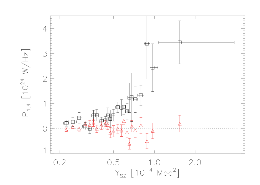
Figure 7: Null test for the PSZ(V) sample, with radio luminosity binned by Comptonization. The radio luminosities derived from the actual PSZ targets are shown as black squares with error bars, where the horizontal bars represent bin widths. Similarly binned radio luminosities derived from fields not a priori associated with clusters of galaxies are shown as red triangles.

Additionally, we test for a possible offset of the measured signal in the vicinity of bright point source. Such bias can be caused by inaccuracies in the removal of compact sources directly in the maps (Section 3.1) or by so-called clean bias (White et al., 1997; Condon et al., 1998). Using randomly chosen NVSS fields (as in the previous null test), we select 200 fields with compact sources brighter than $500$ mJy, centering each field upon the bright compact source, before applying our filtering algorithm. Finally we stack the cleaned maps in two ways: with uniform weighting (to test whether there is a flux bias independent of the peak flux) and weighting by the peak flux (to test whether there is a bias dependent on the magnitude of the compact source). Although we do find a slight bias in the uniformly weighted case, the total (integrated) bias level inside an aperture of one arc-minute is at a level of less than $20~{}\mu$Jy/beam and is thus of no consequence for our results. We find no evidence that the bias scales with the peak flux of the compact source, thus there is no need to consider the peak flux-weighted case separately.

5.6 Individual flux comparison

We conclude this section by comparing individual radio halo flux measurements with previously published results where the latter are available. The published data are collected from Giovannini et al. (2009) and Feretti et al. (2012) (the latter sample containing the former save for one target). One goal of this comparison is to determine whether the limited $uv$-coverage of the NVSS snapshots cause any systematic flux attenuation of these diffuse sources. We carry out the comparison for the union of all our samples, for both flavors of flux extraction after correcting the directly integrated signals for the attenuation effect due to the finite integration aperture, as described in Section 3.2.3. The result of the comparison is summarized in Fig. 8.

$\mathrm{S}_{\mathrm{publ}}$ [mJy]

Figure 8: Comparison of integrated flux density measurements for a sub-sample of the X-ray clusters with the published measurements of Giovannini et al. (2009) and Feretti et al. (2012) denoted collectively here as $S_{\mathrm{publ}}$. Flux density measurements using the direct integration method of this work have been corrected for the finite aperture used for integration (Section 5.2).

We note that while the two flux extraction methods used in this study yield consistent results, there are several cases in which we find results very different from the published values. Considering the different approaches to measuring the radio signals, this is expected. While the results quoted by Giovannini et al. (2009) and Feretti et al. (2012) rely on the visual identification of radio halos and subsequent measurements of the flux within a thus defined aperture, our measurements are based on the assumption of a universal profile for the radio signal, and in addition we do not attempt to visually distinguish radio halos from other potential sources of extended emission (such as mini-halos or radio relics). These effects lead to our method yielding fluxes significantly greater than the previously published radio halo fluxes in many cases.

For other targets (a case in point is Abell 2163) the radio emission is significantly more peaked than the mean profile derived in Section 3.2.1, which leads us to underestimate the flux when using the fitting method. We also note that the NVSS maps are often plagued by side lobe structures and artifacts, especially where there is a bright, peaked radio emission is present. This is the case for Abell 2219, where we recover less than $50\%$ of the flux quoted by Feretti et al. (2012). We also note that our measurements are sensitive to the chosen centroids, which in this work are simply those extracted from the respective cluster catalogs. This can be expected to cause an underestimation in flux with respect to published results, in particular for low-mass and high-redshift targets, where the resulting linear scale is smaller.

A quantitative comparsion of the recovered flux in our two main samples is a potential way of testing for possible biases in the results presented in the next section. In practice, however, this is a difficult test to perform from the available public data. Firstly, published radio halo data are mostly ad-hoc compilations, so the resulting sample will have no specific selection function. In addition, there are no public radio halo data from SZ selected clusters. Secondly, for the objects shared in common between the union of our samples and Feretti et al. (2012), most are also shared between the PSZ and the X-ray samples (23 out of 28 clusters), and therefore the resulting mean flux ratios between our analysis and the published data are thus almost identical for the two sub-samples. We conclude that although we are unlikely to have systematic differences in the flux recovery between the PSZ and X samples, a direct comparison with published radio halo data presently does not offer a conclusive test for such a bias.

6 Results

We now have all the tools in place to approach the main objective of our work, namely to find the correlations between radio halo power and the mass observables ($Y_{\mathrm{SZ}}$ and $L_{\mathrm{X}}$) in our cluster samples and quantify the fraction of clusters that do not follow the main correlation (i.e. consistent with having no radio halo emission). We carry out the regression analysis on the measured radio luminosities found by the two methods described in Section 3.2 and present the results in Section 6.1. We compare our results to the literature in Section 6.2, and discuss the direct scaling of mass and radio halo power in Section 6.3.

Table 3: Best-fit (maximum likelihood) parameters of the power law $P_{\text{1.4~{}GHz}}=A_{\mathrm{lim}}(\frac{x}{x_{\mathrm{lim}}})^{B}$, where $x$ is the mass observable ($Y_{\mathrm{SZ}}$, measured in $10^{-4}~{}\text{Mpc}^{2}$, or $L_{\mathrm{X}}$, measured in $10^{44}~{}\mathrm{erg}~{}\mathrm{s}^{-1}$). $A_{\mathrm{lim}}$ and $x_{\mathrm{lim}}$ are the re-normalized regression parameters as defined in the text. For each cluster sample, the analysis was carried out for the two different flux extraction methods described in the text, and fitted using the mixture model for the dropout population.

Variable mass limit
Sub-sample	Mass	Sub-sample	Flux extraction	Normalization $A_{\mathrm{lim}}$	Power law	Intrinsic	dropout
	limit	size	method	[$10^{24}\mathrm{W}\,\mathrm{Hz}^{-1}$]	slope $B$	scatter $\sigma_{\mathrm{F}}$	fraction $g$
X(V)	$z$-dependent	85	Radial fit	$0.56^{+0.49}_{-0.24}$	$1.13^{+0.27}_{-0.17}$	$0.98^{+0.45}_{-0.20}$	$0.51^{+0.09}_{-0.13}$
X(V)	$z$-dependent	85	Direct integration	$0.37^{+0.43}_{-0.24}$	$1.48^{+0.53}_{-0.30}$	$0.54^{+0.40}_{-0.17}$	$0.70^{+0.07}_{-0.11}$
PSZ(V)	$z$-dependent	89	Radial fit	$0.52^{+0.26}_{-0.12}$	$1.63^{+0.24}_{-0.28}$	$0.82^{+0.39}_{-0.15}$	$0.25^{+0.11}_{-0.13}$
PSZ(V)	$z$-dependent	89	Direct integration	$0.37^{+0.19}_{-0.10}$	$1.75^{+0.32}_{-0.22}$	$0.86^{+0.42}_{-0.17}$	$0.29^{+0.12}_{-0.12}$
Constant mass limit
Sub-ample	Mass	Sub-sample	Flux extraction	Normalization $A_{\mathrm{lim}}$	Power law	Intrinsic	dropout
	limit	size	method	[$10^{24}\mathrm{W}\,\mathrm{Hz}^{-1}$]	slope $B$	scatter $\sigma_{\mathrm{F}}$	fraction $g$
X(C)	$8\times 10^{14}M_{\odot}$	77	Radial fit	$0.33^{+0.68}_{-0.28}$	$1.55^{+0.54}_{-0.48}$	$0.77^{+0.30}_{-0.29}$	$0.58^{+0.12}_{-0.11}$
X(C)	$8\times 10^{14}M_{\odot}$	77	Direct integration	$0.51^{+0.93}_{-0.45}$	$1.31^{+0.65}_{-0.52}$	$0.71^{+0.39}_{-0.22}$	$0.71^{+0.06}_{-0.11}$
PSZ(C)	$8\times 10^{14}M_{\odot}$	79	Radial fit	$0.56^{+0.19}_{-0.12}$	$1.59^{+0.26}_{-0.23}$	$1.14^{+0.26}_{-0.16}$	$0.11^{+0.08}_{-0.11}$
PSZ(C)	$8\times 10^{14}M_{\odot}$	79	Direct integration	$0.50^{+0.18}_{-0.11}$	$1.63^{+0.28}_{-0.20}$	$1.06^{+0.25}_{-0.14}$	$0.18^{+0.10}_{-0.11}$

6.1 Model fit

The results of our likelihood analysis are summarized in Table 3. In order to have physically meaningful and internally comparable values for the power law normalization, we re-scale Equation 6 as

$$y=A_{\mathrm{lim}}\left(\frac{x}{x_{\mathrm{lim}}}\right)^{B}.$$ (12)

The newly defined power-law normalization, $A_{\mathrm{lim}}$, corresponds to the value $x_{\mathrm{lim}}$ of the mass observable, obtained using the definitions in Section 2, for a fixed mass of $M_{500}=6\times 10^{14}M_{\odot}$. Thus, for the X-ray subsamples, $x_{\mathrm{lim}}=3.6\times 10^{44}~{}\mathrm{erg}~{}\mathrm{s}^{-1}$, and for the SZ subsamples $x_{\mathrm{lim}}=0.43\times 10^{-4}~{}\mathrm{Mpc}^{2}$.

The relatively larger uncertainties in the best-fit parameters for the X-ray sub-samples, in spite of sample sizes similar to PSZ, reflect a higher dropout fraction, and thus fewer data points serving to constrain the power law.

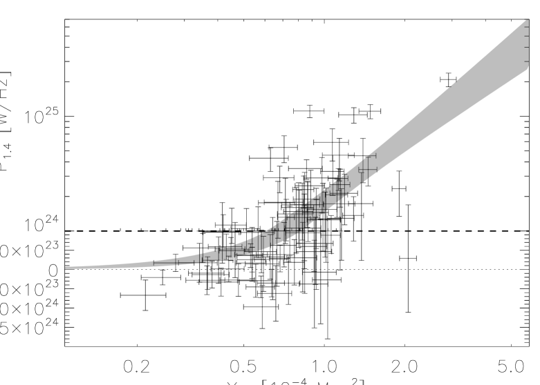
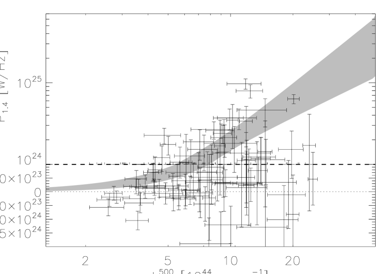
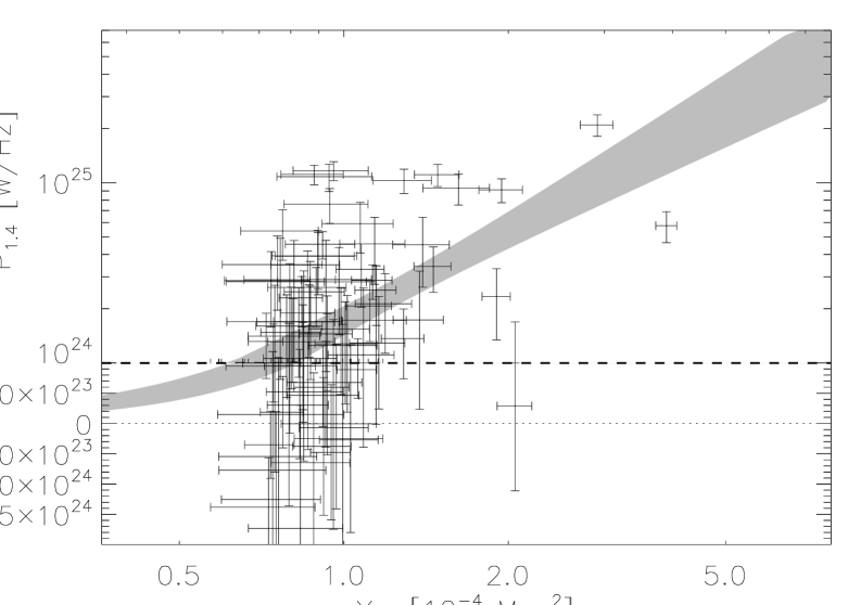
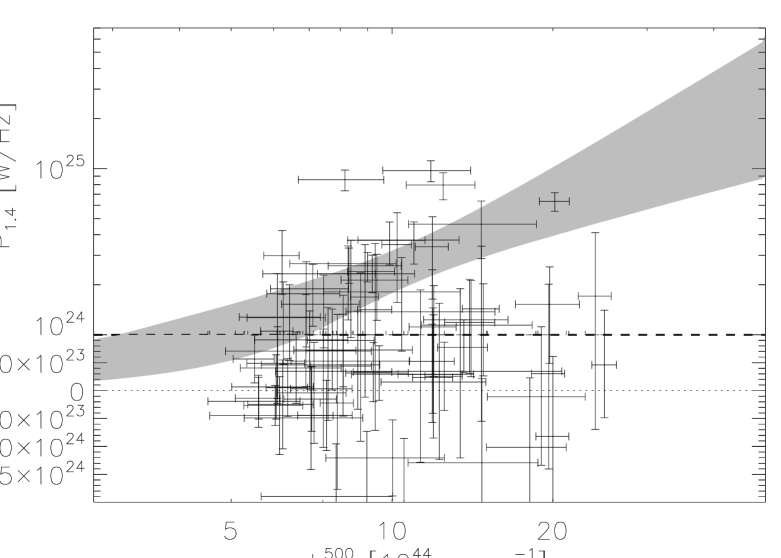
Figure 9: 1.4 GHz radio power plotted against $Y_{\text{SZ}}$ for the PSZ (left column) and X-ray (right column) sub-samples, using the direct integration method for flux extraction. The upper panels show the case for a variable mass limit (PSZ(V) and X(V), respectively), and the lower panels are for a constant mass-cut (PSZ(C) and X(C), respectively). The gray shaded region in each panel represents the 68% confidence region of the best-fit power-law, using the mixture model to account for the off-population as described in the text. Note that the ordinate axes are broken into linear and logarithmic parts.

In Figure 9 we show the radio power versus the mass observable for the different sub-samples, accompanied by the allowed range (at 68% confidence) of power law models. Although the effect of contamination from radio point sources is small, we model the power law and dropout-fraction taking this effect into account as described in Section 5.3. It is clear that most of our radio halo measurements are formally non-detections (the fraction of measurements above a $3\sigma$ threshold being in the approximate range of 20%-35%). We refer to Section 5.6 for a quantitative comparison with published results. We visualize the posterior likelihood distributions by marginalizing over the four regression parameters (the slope $B$ and normalization $A_{\mathrm{lim}}$, the intrinsic scatter in the radio power $\sigma_{F}$, and the dropout fraction $g$), as displayed in Figures 10 and 11.

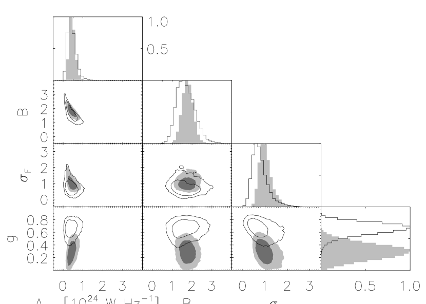
Figure 10: Marginalized posterior probability distributions for the maximum-likelihood analysis for the sub-samples with redshift dependent mass limits. Filled (gray) and black contours represent the results for the PSZ(V) and X(V) sub-samples (direct integration method), respectively. The contours encompass 68% and 95% of all sampled points in the posterior, marginalized over the other parameters. Also shown are histograms representing the (normalized) marginalized distributions of single parameters of the fit.

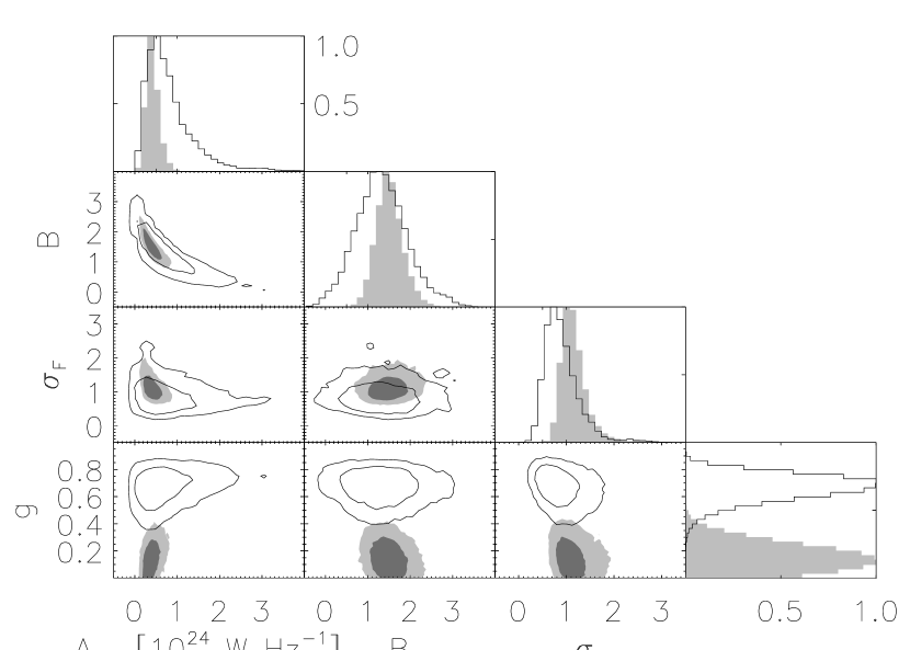
Figure 11: As figure 10, but for the PSZ(C) (gray, filled contours) and X(C) (solid black contours) sub-samples, selected by a constant mass limit.

The model parameters for the power law are essentially consistent between the different samples. This is expected, since the core-excised soft band X-ray luminosity scales almost linearly with the integrated SZ signal (e.g. $Y_{\mathrm{SZ}}\propto L_{\mathrm{X}}^{1.14\pm 0.08}$, Arnaud et al., 2010), and we do not expect to see the small difference in the power-law coefficients given the large statistical errors (see Section 6.3 for a direct comparison in terms of mass scaling). The dropout fractions, however, are generally inconsistent between the SZ and X-ray selected samples. This is especially the case comparing the constant-mass selected sub-samples.

It is conceivable that differences in the redshift distribution of clusters can cause the observed differences in the dropout fraction. Although the redshift distributions of the PSZ and X-ray sub-samples are very similar below $z<0.3$, as indicated in Fig. 2, the higher number of $z>0.3$ objects in the PSZ selection is a cause for concern. It remains a possibility that in the high redshift universe the merging fraction is higher and hence the PSZ sub-samples show an increased occurrence of radio halos. To test this, we re-perform the analysis limiting the samples to redshifts below $z=0.3$. Although the parameter uncertainties increase due to the lower samples sizes, the results are in general agreement with the above. We find $g=0.66^{+0.08}_{-0.22}$ and $g=0.25^{+0.11}_{-0.21}$ for the X(V) and PSZ(V) samples, respectively, and $g=0.53^{+0.13}_{-0.20}$ and $g=0.00^{+0.11}_{-0.00}$ for the corresponding (C) samples. We also find consistent slopes and normalizations in each case. Finally, we note that the intrinsic scatter is found to be very large (close to 100%) in all samples, consistent with the estimates of B12.

6.2 Comparison with published results

We now compute weighted averages of the derived radio halo luminosities and compare to published correlations with X-ray and SZ mass observables. We divide each sample into two equally large (by number of targets) mass bins, and average the radio luminosities weighted by the inverse square of their uncertainties. In Fig. 12 we compare our result from the PSZ sample with the radio/SZ correlation of B12, based on the compilations of Brunetti et al. (2009) and Giovannini et al. (2009). As expected, the mean values are generally consistent with the correlation of the ”radio-on” population of B12, since the dropout fraction in the PSZ sample is small (or consistent with zero at the high mass end). In the low mass bin the fraction of dropouts is higher, hence the mean value lies below the 68% confidence region of the radio-halo only regression (indicated by the gray band in Fig. 12). This result again illustrates that there is no net bias in the radio halo flux measurements from our method compared to previous studies.

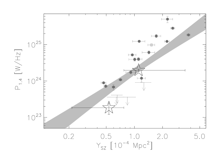
Figure 12: Weighted mean values (open stars) of $Y_{\text{SZ}}$ and $P_{1.4\text{GHz}}$ after dividing the PSZ(V) sample (direct integration method) into two bins equal by number of targets. The 68% confidence region of the power law fit of this work is indicated in gray. Also indicated are previously known radio halos (filled circles), mini-halos (open circles) and upper limits (arrows), selected from Brunetti et al. (2009) based on cross-selection with PSZ.

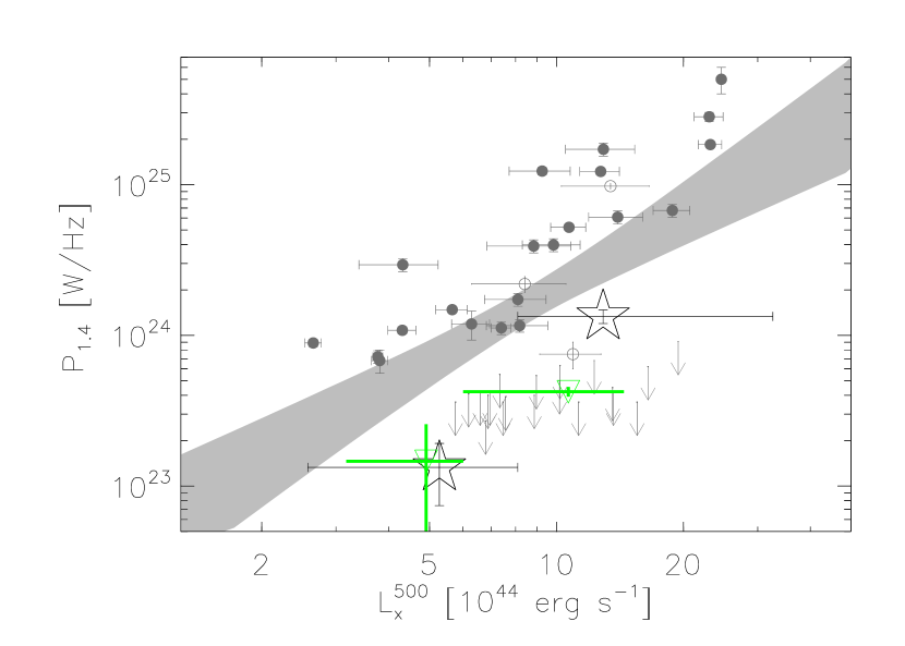
Figure 13: As Figure 12, but for the X(V) sample (direct integration method). All radio halos (filled circles), mini-halos (open circles) and upper limits (arrows) of Brunetti et al. (2009) are indicated. Also indicated are the measurements of Brown et al. (2011) (green triangles) in two bins of X-ray luminosity.

For the correlation with $L_{\mathrm{X}}$ we again use the Brunetti et al. (2009) sample that includes radio halos, mini-halos and upper limits on non-detections. We compare these results to the mean signals in our two $L_{\mathrm{X}}$ bins (Fig. 13), and find that they are below the 68% confidence interval of the radio halo correlation found in Section 6. This is expected since the mean values are an average of the “on” and “off” populations (the latter being approximately $\sim 70$% in the X-ray selection). In Fig. 13 we also show the results of Brown et al. (2011), from stacking of SUMSS radio maps in a sample of X-ray clusters. We find that the signal in the low-$L_{\mathrm{X}}$ bin from Brown et al. is consistent with our measurement, but in the higher $L_{\mathrm{X}}$ bin their upper limit is significantly lower than the mean signal derived from our analysis.

Since the mean values from the stacked radio images of X-ray clusters of Brown et al. (2011) have been claimed as a detection of the radio halo “off-state”, the factor $\sim$3 discrepancy with our mean value in the high $L_{\mathrm{X}}$ bin requires some clarification. We suggest this difference is likely caused by a combination of several factors, both in the sample selection and map filtering procedures. The Brown et al. sample is not X-ray flux limited and hence their high-$L_{\mathrm{X}}$ sample may contain several lower mass objects with peaked X-ray emission (see Section 7.2). Their sample is also cut to approximately two-thirds of its original number by a criterion that relates the peak flux in each field with cluster mass, and hence can systematically remove some of the brightest radio halos as well as massive, cool-core clusters with a central AGN. On the map filtering side, the use of the multi-scale spatial filter of Rudnick (2002) can cause an under-estimation of radio halo flux if emission is highly clumped (see the discussion in Rudnick & Lemmerman, 2009). We tested the performance of the Rudnick (2002) filter on our simulated maps and found it to be more strongly affected by residual point source flux and substructures. Finally, the use of a fixed filtering scale of 600 kpc in Brown et al. for all clusters will create a bias against smaller radio halos in low-mass objects (conversely, removed the contribution of mini-halos that can potentially contaminate our results). Based on these considerations we argue that the mean flux of radio halos in X-ray luminous clusters might have been under-estimated by Brown et al.

6.3 $P_{\mathrm{1.4~{}GHz}}-M_{500}$ scaling

Our measured scaling of the radio halo luminosities with mass observables lead to consistent results between the SZ and X-ray selected samples. We estimate the mass scaling of radio halos by measuring the slope of the $P_{\mathrm{1.4~{}GHz}}-M_{500}$ correlation directly from the posterior distribution of $Y_{\mathrm{SZ}}-P_{\mathrm{1.4~{}GHz}}$ and $L_{\mathrm{X}}-P_{\mathrm{1.4~{}GHz}}$ slopes presented in the previous section, in conjunction with the mass-observable scaling relations discussed in Section 2. The results are presented in Table 4 and graphically in Figure 14.

Table 4: Slope of the $P_{\mathrm{1.4~{}GHz}}-M_{500}$ scaling: $P_{\mathrm{1.4~{}GHz}}\propto M_{500}^{\gamma}$

Sub-sample	Flux extraction	Power law
sample	method	slope $\gamma$
X(V)	Radial fit	$1.96^{+0.50}_{-0.32}$
X(V)	Direct integration	$2.57^{+0.97}_{-0.52}$
PSZ(V)	Radial fit	$2.84^{+0.46}_{-0.50}$
PSZ(V)	Direct integration	$3.10^{+0.57}_{-0.40}$
X(C)	Radial fit	$2.68^{+0.98}_{-0.82}$
X(C)	Direct integration	$2.78^{+1.13}_{-0.88}$
PSZ(C)	Radial fit	$2.78^{+0.49}_{-0.40}$
PSZ(C)	Direct integration	$2.88^{+0.50}_{-0.36}$

Figure 14: Slope of the $P_{\mathrm{1.4~{}GHz}}-M_{500}$ scaling: $P_{\mathrm{1.4~{}GHz}}\propto M_{500}^{\gamma}$, from the various flavors of sample selection and flux extraction methods. The B12 result is included for comparison.

The current results are mostly consistent at one-sigma level with the one found by B12 using an ad-hoc selection of known radio halos present in the ESZ catalog ($P_{1.4}\propto M_{\mathrm{vir}}^{3.4\pm 0.4}$). There is, however, an indicative trend towards a flatter $P_{\mathrm{1.4~{}GHz}}-M_{500}$ correlation, as each of the sub-sample and flux estimation method shows preference towards a smaller value than B12. The presence of many high-mass clusters in the ad-hoc B12 selection and possible absence of non-detections in the literature may be responsible for this bias. We also note that the secondary or hadronic models predict a shallower mass correlation of radio halo power than the primary or re-acceleration ones (e.g. Kushnir, Katz & Waxman, 2009; Cassano et al., 2013), but we do not dwell further on this difference given its low statistical significance. We also do not attempt to scale the $Y_{\mathrm{SZ}}$ values from the PSZ catalog to inside the radio halo radius (as was done in B12 to obtain a roughly linear correlation between the SZ and radio signals) since neither of our flux extraction methods allow a direct measurement of the radio halo radius from the NVSS data.

The scaling of the radio halo power with the total cluster mass is a more useful indicator for predicting radio halo counts from cosmological-scale simulations. Such simulations are still in their early stages, and the large number of free parameters need to be matched against observations. Sutter & Ricker (2012), for example, showed that the slope of the $P_{1.4}-M_{\mathrm{vir}}$ correlation can be useful to distinguish different models of radio halo origins. Even though the uncertainties in the scaling relation presented in our work will not help in breaking most of the parameter degeneracies, some models, e.g. those with high magnetic field strengths, can be ruled out at high significance.

7 Discussion

The main result of our analysis is a statistically significant difference in the number of “radio quiet” clusters in the SZ and X-ray selected samples. Having established that our radio flux measurements are not subject to any map filtering bias or other systematic artifacts, we turn our attention to a qualitative understanding of this difference. We begin by considering biases arising from the presence or absence of cool-core clusters in different types of samples. Finding that such bias is unlikely to be the sole contributor to the observed selection difference, we put forward the different time evolution of the SZ and X-ray signals during cluster mergers as a more likely cause. We offer some predictions based on the latter hypothesis, and conclude this section with a crude estimate of the expected number of radio halos in the sky.

7.1 Bias due to cool cores

In our earlier work (B12) using the Planck ESZ catalog, we proposed the over-abundance of cool-core clusters in X-ray selected samples as a possible reason for strong bi-modality. Cool core clusters are predominantly relaxed systems which generally do not harbor giant radio halos, although they often exhibit radio mini-halos at their centers. The bias towards cool core clusters in X-ray selected samples is well known. Eckert, Molendi & Paltani (2011) showed that up to $\sim 30\%$ of the strong cool-core objects should be removed from a given X-ray flux-limited sample. Inclusion of several lower mass objects near the mass limit of X-ray selected samples will thus create a bias towards radio quiet systems.

An objection to the above argument is that a strong cool-core bias will be more prominent at the low-$L_{\mathrm{X}}$ end, and thus the massive clusters considered in our study should only be moderately affected. The significant discrepancy in the radio halo hosting population between the X-ray and SZ selected clusters is difficult to explain solely from the contamination of a few less massive cool-core clusters near the X-ray mass selection threshold.

That being said, the appearance of cool cores will boost the X-ray luminosity in a cluster disproportionate to its mass, thereby “enhancing” the bi-modal division which is already prominent in the X-ray selection. The recent results of Cassano et al. (2013) support this scenario: after excising the core emission in an X-ray selected cluster sample these authors still find a bi-modal division in the radio/X-ray correlation, but it is less prominent compared to the core-inclusive values. This result is fully consistent with our finding of roughly 65% radio dropouts in the X-ray selection. Note, however, that the use of a lower scatter mass proxy (e.g. $Y_{X}$) in a thus selected sample will lessen the visual perception of bi-modality.

Conversely, it can be argued that the PSZ cluster catalog is biased against cool-core systems due to their radio AGN contamination. Cool core clusters tend to be associated with a radio AGN at their center (e.g. Sun, 2009; Mittal et al., 2009), which in principle can offset or completely cancel the SZ decrement. However, at the high S/N level that our PSZ clusters are selected such a contamination is expected to be negligible. The PSZ catalog does contain several high-mass, cool core systems, and the Planck team identifies only 11 clusters with a central AGN that are present in the MCXC catalog but not in the PSZ selection (Planck Collaboration, 2013b). Of these only 5 objects satisfy our selection criteria, a small fraction compared to our sample sizes. It is more likely that the expected SZ signals from these objects are erroneously over-predicted based on their high $L_{\mathrm{X}}$ values, rather than the SZ signal being contaminated by a radio AGN. In general, it has been shown from simulations (Sehgal et al., 2010) and direct observations (Sayers et al., 2013) that radio AGN contamination in SZ surveys is well below 5% for the high-significance detections. Thus we can rule out any significant bias against cool core objects in the high signal-to-noise PSZ clusters used in our study.

We conclude that even though the X-ray selected sub-samples can contain several lower mass, X-ray luminous cool core clusters, these objects alone are unlikely to create the significant difference in the radio halo occupancy that we find between SZ and X-ray selection. If the mass selection threshold is decreased further, the cool core bias will create an increasing dropout fraction in the X-ray selection (which is indeed observed, see e.g. Kale et al., 2013), but at the high-mass end its impact will be less severe. To understand our results, we therefore take a closer look at how the SZ and X-ray mass observables change with time during mergers when the radio halos are supposedly at their brightest.

7.2 X-ray and SZ signal during mergers

Simulations indicate that the merger related boost in the SZ signal is much smaller than that of the X-ray signal. We use the simulation data of Poole et al. (2007) as an illustration of this point, showing in Fig.15 the time variation of the integrated X-ray bolometric luminosity and the SZ signal inside $r_{500}$ during and after mergers. The examples are for head-on mergers, with mass ratios 1:1. 3:1 and 10:1, respectively. The SZ and X-ray signals are normalized with respect to their final values, scaled from the initial ones through observed correlations (see Poole et al., 2007, for details). These controlled merger simulations highlight the less severe fluctuations of the SZ signal during and after the merger process, and its tendency to remain close to the predicted scaling values in the subsequent relaxed phase (red lines in Fig. 15). More importantly for our purpose, the integrated SZ signal, in contrast to the X-ray luminosity, does not show a drop in intensity right after the cluster core passage. The drop in central density in a disruptive merger is compensated by a rise in the gas temperature, keeping the pressure close to its equilibrium value.

Under the assumption that radio halos are fueled by post-merger turbulence and energy dissipation, the drop ($\sim$50% or more) in the X-ray luminosity is likely to create a bias against radio halo clusters in X-ray selected samples. We note that the $L_{\mathrm{X}}$ de-boost phase can last several Gyr, possibly covering the entire radio halo lifetimes. On the other hand, there is an indicative bias towards finding radio halos in SZ selection, as the delayed boost in the SZ signal during mergers can preferentially aid the detection of radio halo clusters. However, the latter bias should be small if the duration of the radio halo is longer than the typical timescale of the SZ extended boost, which is on the order of 1 Gyr.

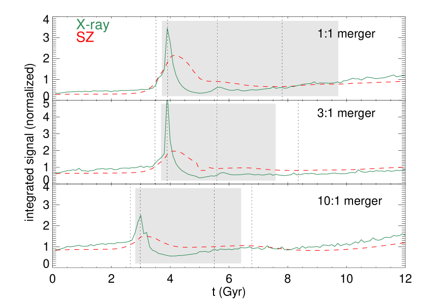
Figure 15: Relative changes in SZ and X-ray observables during cluster mergers (simulation data from Poole et al., 2007). The red-dashed and green-solid lines denote $Y_{\mathrm{SZ}}$ and $L_{\mathrm{X}}$ inside $r_{500}$, respectively. The signals are normalized to their final equilibrium values computed from the observed scaling and final mass. The vertical dotted lines, from left to right, denote the times of virial crossing, first core crossing (first pericenter), second core crossing (second pericenter), and the time when the remnants will appear as a relaxed object in X-rays. The gray shaded regions are meant as tentative illustrations of radio halo lifetimes during mergers.

The opposing trend between cluster X-ray luminosity and the radio halo activity has also been demonstrated recently through high-resolution MHD simulations (Donnert et al., 2013), and we identify this as a principal cause for the observed selection difference between high-mass SZ and X-ray clusters. For illustration, we indicate tentative radio halo lifetimes in Fig. 15 as gray shaded regions, where the lifespans are chosen to be proportional to the total mass (we emphasize that this illustrative example is not based on any simulation results). An immediate consequence of the above argument is the prediction of radio halos in X-ray under-luminous late-merger clusters. Indeed such clusters have been reported (see Giovannini et al., 2011), but the numbers are small, as expected, since the selection was done in X-rays. As blind detections of radio halos from future radio surveys will be followed-up through X-ray and SZ observations, the radio X-ray correlation is thus expected to broaden significantly, while the radio SZ correlation will remain less affected.

The rapid rise in X-ray luminosity, lasting for only $\sim 0.5$ Gyr, can also explain those rare merging systems that do not host radio halos, for example Abell 2146 (Russell et al., 2011). If the onset of giant radio halos is not instantaneous and the radio brightness reaches its maximum after the cluster core crossing (second vertical dotted line from left in Fig. 15), then for a short fraction of their life clusters can be significantly X-ray bright but radio under-luminous. Again, the same offset will cause a less severe scatter in the radio-SZ correlation since the boost in the SZ signal during mergers is less prominent, and occurs at a slightly delayed time-scale that potentially corresponds better to the peak in the radio halo flux.

7.3 Implications for future radio surveys

Radio halos are challenging to detect from blind radio observations: they are diffuse, low-brightness objects with considerable sub-structure, often confused with radio relics and even extended radio galaxies. At low redshifts their Mpc scale emission cannot be imaged with most radio interferometers, and at high redshifts their surface brightness drops rapidly due to cosmological dimming and the K-correction. Nevertheless, several upcoming low-frequency radio surveys, such as LOFAR and the SKA pathfinder experiments which will become operational in the next decade, can address these observational challenges. At 1.4 GHz, the ASKAP/EMU survey (Norris et al., 2011) will map the radio sky with roughly 10^′′ resolution and 40 times better sensitivity than the NVSS, and a similar capability is also expected from the WODAN project (Röttgering et al., 2011).

Consequently there is a revived interest in observing radio halos (and relics) with these instruments, but the theoretical predictions are uncertain. Based on the observed low number count of radio halos in X-ray selected clusters, Cassano et al. (2012) predicted up to $100-200$ objects in the whole sky with 1.4 GHz fluxes $\gtrsim$ 1 mJy. There is much uncertainty in these numbers as there are several model parameters that can vary by a wide margin (Cassano et al., 2010). There is a similar situation in the cosmological simulations for radio halo formation (Sutter & Ricker, 2012), which are at an early stage but tend to predict more radio halos than re-acceleration based models. In light of this, it is interesting to make a rough estimate of the radio halo count in the entire sky based on our dropout fraction in SZ selected samples.

At the constant mass cut used for the PSZ(C) and X(C) samples, $M_{500}>8\times 10^{14}$ M_⊙, there are over 200 clusters in the entire sky (computed using the mass function of Tinker et al., 2008), with the majority below redshift $z=0.6$. This number increases to over 1800 for a mass cut of $M_{500}>5\times 10^{14}$ M_⊙, corresponding to the low-$z$ completeness limit of the Planck cosmological sample. In the redshift range $z<0.5$ there are roughly 1000 clusters in the entire sky, and Planck is expected to have most of these massive objects in its final data release. If we use the dropout fraction from the PSZ(V) sample, $g=0.25\pm 0.12$ using the radial fit method, we can expect roughly $750\pm 120$ radio halos in the sky in this redshift range. This is roughly a factor of 5 more than the current predictions at 1.4 GHz for the ASKAP/EMU and WODAN surveys (Cassano et al., 2012).

The crucial information needed to make a more realistic prediction of radio halo counts in the sky is how the dropout fraction varies with cluster mass. We have been unable to probe the lower mass domain as our selection is based on the Planck PSZ catalog of the most massive objects in the universe. The noisy NVSS data also prohibits such an analysis as the radio power decreases rapidly with cluster mass. These intermediate- to low-mass objects will form the bulk of radio halo detections in the future radio surveys at 1.4 GHz and at low frequencies, so future work must address this mass-dependence issue observationally by dedicated follow-up observation of several tens of clusters. Finally, if a large fraction of clusters are found to be host to radio halos at all masses, they can effectively be used to probe the increasing merger rate of cluster-size dark matter halos through the cosmic time, an important test for the concordance model of cosmology.

8 Summary and conclusions

We have measured the rate of occurrence of radio halos in galaxy clusters and their correlation with cluster mass observables. We constructed two main cluster samples: an X-ray selected sample based on the REFLEX, BCS/eBCS, NORAS and MACS catalogs, and an SZ selected sample based on the Planck PSZ catalog. The cuts in the X-ray luminosity and the integrated Comptonization parameters were chosen to ensure near identical mass limits. The samples were cross-correlated with the NRAO VLA Sky Survey (NVSS) data at 1.4 GHz to search for diffuse, central radio emission not associated with radio galaxies or other non-central diffuse emission. The most important points of our analysis can be summarized as follows:

• We iteratively remove all compact sources from the maps, so as to extract the central diffuse emission with a wide range of morphologies and scales. We attempt to minimize the contribution from radio relics and mini-halos, although some contamination cannot be ruled out.

• We employ two independent methods for radio flux extraction, based on a average model fit and a direct integration. The flux extraction is carried out within a radius $0.5\times r_{500}$, and we account for the missing flux outside this region using a common stacked radial profile (our results do not depend on this flux extrapolation). Due to the large uncertainties, the majority of the individual signals are consistent with zero at the $3\sigma$ level.

• We model the relation between radio power and mass observables with a power law, accounting for intrinsic scatter in the measurements, uncertainties in the dependent and independent variables, and a dropout fraction quantifying the fraction of objects not hosting a central, diffuse radio emission component.

• We run an extensive set of simulations to determine any biases that might occur from the filtering method, residual flux from bright sources, a point source population below the confusion limit, or the regression analysis.

We summarize the main conclusions of our work:

1. The SZ and X-ray selected cluster samples both show the presence of a radio halo population, whose individual and averaged flux measurements are generally consistent with previously published results. The scaling of the radio halo power with the total cluster mass from these two samples are consistent. The intrinsic scatter is found to be large.

2. The SZ selected samples based on the Planck PSZ catalog yield a low radio halo dropout fraction (i.e. clusters hosting no radio halos). For a sub-sample built from the redshift-dependent mass limit similar to the Planck cluster cosmology sample, the dropout fraction is roughly $30\pm 10\%$. For a constant mass-cut PSZ sub-sample with masses $M_{500}>8\times 10^{14}$ M_⊙, the dropout fraction is found to be consistent with zero at approximately $15\pm 10$%, suggesting a nearly complete occurrence rate at the very high-mass end.

3. The situation is different in the case of X-ray selection. Using a complete sample based on the REFLEX, BCS/eBCS, NORAS and MACS cluster catalogs and the same redshift-dependent mass limit, the dropout fraction in X-ray selected clusters is roughly $60\pm 10$%. The fraction is effectively unchanged in the constant mass selection. These numbers are fully consistent with the general view that radio halos are rare objects, with roughly 70% of the high X-ray luminosity clusters ($L_{\mathrm{X}}>5\times 10^{44}$ erg/s) being in the radio “off-state”.

4. The difference between the SZ and X-ray selections is likely a combination of two effects: dissimilar scatter in these two mass observables during cluster mergers, and a cool-core bias in X-ray flux limited samples. The first argument can be used to explain the absence of radio halos in some early mergers, and to predict a large number of radio halos in clusters that are X-ray under-luminous in the late merger phase.

References

- Arnaud et al. (2010) Arnaud M., Pratt G. W., Piffaretti R., Böhringer H., Croston J. H., Pointecouteau E., 2010, \aap, 517, A92
- Basu (2012) Basu K., 2012, \mnras, 421, L112
- Becker, White & Helfand (1995) Becker R. H., White R. L., Helfand D. J., 1995, \apj, 450, 559
- Blasi & Colafrancesco (1999) Blasi P., Colafrancesco S., 1999, Astroparticle Physics, 12, 169
- Böhringer et al. (2004) Böhringer H. et al., 2004, \aap, 425, 367
- Böhringer et al. (2000) Böhringer H. et al., 2000, \apjs, 129, 435
- Bonafede et al. (2009) Bonafede A., Giovannini G., Feretti L., Govoni F., Murgia M., 2009, \aap, 494, 429
- Brown et al. (2011) Brown S., Emerick A., Rudnick L., Brunetti G., 2011, \apjl, 740, L28
- Brunetti et al. (2009) Brunetti G., Cassano R., Dolag K., Setti G., 2009, \aap, 507, 661
- Brunetti et al. (2001) Brunetti G., Setti G., Feretti L., Giovannini G., 2001, \mnras, 320, 365
- Buote (2001) Buote D. A., 2001, \apjl, 553, L15
- Cassano et al. (2012) Cassano R., Brunetti G., Norris R. P., Röttgering H. J. A., Johnston-Hollitt M., Trasatti M., 2012, \aap, 548, A100
- Cassano et al. (2010) Cassano R., Brunetti G., Röttgering H. J. A., Brüggen M., 2010, \aap, 509, A68
- Cassano et al. (2007) Cassano R., Brunetti G., Setti G., Govoni F., Dolag K., 2007, \mnras, 378, 1565
- Cassano et al. (2013) Cassano R. et al., 2013, \apj, 777, 141
- Condon et al. (1998) Condon J. J., Cotton W. D., Greisen E. W., Yin Q. F., Perley R. A., Taylor G. B., Broderick J. J., 1998, \aj, 115, 1693
- Coppin et al. (2011) Coppin K. E. K. et al., 2011, \mnras, 416, 680
- Dennison (1980) Dennison B., 1980, \apjl, 239, L93
- Donnert et al. (2013) Donnert J., Dolag K., Brunetti G., Cassano R., 2013, \mnras, 429, 3564
- Ebeling et al. (2000) Ebeling H., Edge A. C., Allen S. W., Crawford C. S., Fabian A. C., Huchra J. P., 2000, \mnras, 318, 333
- Ebeling et al. (1998) Ebeling H., Edge A. C., Bohringer H., Allen S. W., Crawford C. S., Fabian A. C., Voges W., Huchra J. P., 1998, \mnras, 301, 881
- Ebeling, Edge & Henry (2001) Ebeling H., Edge A. C., Henry J. P., 2001, \apj, 553, 668
- Eckert, Molendi & Paltani (2011) Eckert D., Molendi S., Paltani S., 2011, \aap, 526, A79
- Enßlin et al. (2011) Enßlin T., Pfrommer C., Miniati F., Subramanian K., 2011, \aap, 527, A99
- Ensslin et al. (1998) Ensslin T. A., Biermann P. L., Klein U., Kohle S., 1998, \aap, 332, 395
- Feretti et al. (2012) Feretti L., Giovannini G., Govoni F., Murgia M., 2012, \aapr, 20, 54
- Giovannini et al. (2009) Giovannini G., Bonafede A., Feretti L., Govoni F., Murgia M., Ferrari F., Monti G., 2009, \aap, 507, 1257
- Giovannini et al. (2011) Giovannini G., Feretti L., Girardi M., Govoni F., Murgia M., Vacca V., Bagchi J., 2011, \aap, 530, L5
- Govoni et al. (2001) Govoni F., Enßlin T. A., Feretti L., Giovannini G., 2001, \aap, 369, 441
- Govoni et al. (2004) Govoni F., Markevitch M., Vikhlinin A., van Speybroeck L., Feretti L., Giovannini G., 2004, \apj, 605, 695
- Hoeft & Brüggen (2007) Hoeft M., Brüggen M., 2007, \mnras, 375, 77
- Hoeft et al. (2011) Hoeft M., Nuza S. E., Gottlöber S., van Weeren R. J., Röttgering H. J. A., Brüggen M., 2011, Journal of Astrophysics and Astronomy, 32, 509
- Hogg, Bovy & Lang (2010) Hogg D. W., Bovy J., Lang D., 2010, ArXiv e-prints
- Kale et al. (2013) Kale R., Venturi T., Giacintucci S., Dallacasa D., Cassano R., Brunetti G., Macario G., Athreya R., 2013, \aap, 557, A99
- Kelly (2007) Kelly B. C., 2007, \apj, 665, 1489
- Kushnir, Katz & Waxman (2009) Kushnir D., Katz B., Waxman E., 2009, \jcap, 9, 24
- Liang et al. (2000) Liang H., Hunstead R. W., Birkinshaw M., Andreani P., 2000, \apj, 544, 686
- Lin & Mohr (2004) Lin Y., Mohr J. J., 2004, \apj, 617, 879
- Mittal et al. (2009) Mittal R., Hudson D. S., Reiprich T. H., Clarke T., 2009, \aap, 501, 835
- Norris et al. (2011) Norris R. P. et al., 2011, \pasa, 28, 215
- Nuza et al. (2012) Nuza S. E., Hoeft M., van Weeren R. J., Gottlöber S., Yepes G., 2012, \mnras, 420, 2006
- Petrosian (2001) Petrosian V., 2001, \apj, 557, 560
- Piffaretti et al. (2011) Piffaretti R., Arnaud M., Pratt G. W., Pointecouteau E., Melin J.-B., 2011, \aap, 534, A109
- Planck Collaboration (2011a) Planck Collaboration, 2011a, \aap, 536, A8
- Planck Collaboration (2011b) Planck Collaboration, 2011b, \aap, 536, A11
- Planck Collaboration (2013a) Planck Collaboration, 2013a, ArXiv:astro-ph/1303.5080
- Planck Collaboration (2013b) Planck Collaboration, 2013b, ArXiv:astro-ph/1303.5089
- Poole et al. (2007) Poole G. B., Babul A., McCarthy I. G., Fardal M. A., Bildfell C. J., Quinn T., Mahdavi A., 2007, \mnras, 380, 437
- Röttgering et al. (2011) Röttgering H. et al., 2011, Journal of Astrophysics and Astronomy, 32, 557
- Rudnick (2002) Rudnick L., 2002, \pasp, 114, 427
- Rudnick & Lemmerman (2009) Rudnick L., Lemmerman J. A., 2009, \apj, 697, 1341
- Russell et al. (2011) Russell H. R. et al., 2011, \mnras, 417, L1
- Sayers et al. (2013) Sayers J. et al., 2013, \apj, 764, 152
- Schlickeiser, Sievers & Thiemann (1987) Schlickeiser R., Sievers A., Thiemann H., 1987, \aap, 182, 21
- Schuecker et al. (2001) Schuecker P., Böhringer H., Reiprich T. H., Feretti L., 2001, \aap, 378, 408
- Sehgal et al. (2010) Sehgal N., Bode P., Das S., Hernandez-Monteagudo C., Huffenberger K., Lin Y.-T., Ostriker J. P., Trac H., 2010, \apj, 709, 920
- Skillman et al. (2011) Skillman S. W., Hallman E. J., O’Shea B. W., Burns J. O., Smith B. D., Turk M. J., 2011, \apj, 735, 96
- Sommer et al. (2011) Sommer M. W., Basu K., Pacaud F., Bertoldi F., Andernach H., 2011, \aap, 529, A124
- Sun (2009) Sun M., 2009, \apj, 704, 1586
- Sunyaev & Zeldovich (1980) Sunyaev R. A., Zeldovich I. B., 1980, \araa, 18, 537
- Sunyaev & Zeldovich (1972) Sunyaev R. A., Zeldovich Y. B., 1972, \aap, 20, 189
- Sutter & Ricker (2012) Sutter P. M., Ricker P. M., 2012, \apj, 759, 92
- Tinker et al. (2008) Tinker J., Kravtsov A. V., Klypin A., Abazajian K., Warren M., Yepes G., Gottlöber S., Holz D. E., 2008, \apj, 688, 709
- van Weeren et al. (2011a) van Weeren R. J., Brüggen M., Röttgering H. J. A., Hoeft M., 2011a, \mnras, 418, 230
- van Weeren et al. (2011b) van Weeren R. J., Brüggen M., Röttgering H. J. A., Hoeft M., Nuza S. E., Intema H. T., 2011b, \aap, 533, A35
- Venturi et al. (2008) Venturi T., Giacintucci S., Dallacasa D., Cassano R., Brunetti G., Bardelli S., Setti G., 2008, \aap, 484, 327
- Wen & Han (2013) Wen Z. L., Han J. L., 2013, \mnras, 436, 275
- White et al. (1997) White R. L., Becker R. H., Helfand D. J., Gregg M. D., 1997, \apj, 475, 479