Measuring capital market efficiency: Long-term memory, fractal dimension and approximate entropy

Abstract

We utilize long-term memory, fractal dimension and approximate entropy as input variables for the Efficiency Index [Kristoufek & Vosvrda (2013), Physica A 392]. This way, we are able to comment on stock market efficiency after controlling for different types of inefficiencies. Applying the methodology on 38 stock market indices across the world, we find that the most efficient markets are situated in the Eurozone (the Netherlands, France and Germany) and the least efficient ones in the Latin America (Venezuela and Chile).

1 Introduction

Efficient markets hypothesis (EMH) is one of the cornerstones of the modern financial economics. Since its introduction in 1960s Fama1965 ; Samuelson1965 ; Fama1970 , EMH has been a controversial topic. Nonetheless, the theory still remains a stable part of the classical financial economics. Regardless of its definition via a random walk Fama1965 or a martingale Samuelson1965 , the main idea of EMH is that risk-adjusted returns cannot be systematically predicted and there can be no long-term profits above the market profits assuming the same risk. The EMH definition is also tightly connected with a notion of rational homogenous agents and Gaussian distribution of returns. Both these assumptions have been widely disregarded in the literature Cont2001 .

In the econophysics literature, EMH has been most frequently studied with respect to the correlation structure of the series. There are several papers ranking various financial markets with respect to their efficiency. Research group around Di Matteo DiMatteo2003 ; DiMatteo2005 ; DiMatteo2007 finds that the correlations structure of various assets (stocks, exchange rates and interest rates) is connected to the development of the specific countries and stock markets. The importance of long-term memory and multifractality in the financial series is then further discussed in the subsequent research of the group Barunik2012 ; Morales2012 ; Morales2013 . In the series of papers, Cajueiro & Tabak Cajueiro2004 ; Cajueiro2004a ; Cajueiro2004b ; Cajueiro2005 study the relationship between the long-term memory parameter $H$ and development stages of the countries’ economy. Both groups find interesting results connecting persistent (long-term correlated) behavior to the least developed markets but also anti-persistent behavior for the most developed ones. Lim Lim2007 investigates how the ranking of stock markets based on Hurst exponent evolves in time and reports that the behavior can be quite erratic. Zunino et al. Zunino2010 utilize entropy to rank stock markets to show that the emergent/developing markets are indeed less efficient than the developed ones. Even though the ranking is provided in these studies, the type of memory taken into consideration (either long-term memory or entropy/complexity) is limited and treated separately.

In this paper, we utilize the Efficiency Index proposed by Kristoufek & Vosvrda Kristoufek2013 incorporating long-term memory, fractal dimension and entropy to control for various types of correlations and complexity using a single measure. Basing the definition of the market efficiency simply on no correlation structure, we can state the expected values of long-term memory, fractal dimension and entropy for the efficient market to construct an efficiency measure based on a distance from the efficient market state. Introduction of the entropy measure into the Efficiency Index is novel compared to the original one Kristoufek2013 and it substitutes the short-term memory effect of the Index which turned out to be a rather weak component of the Index. Short-term memory inefficiency is still controlled for by inclusion of the fractal dimension. As it turns out, the inclusion of the entropy measure has a strong effect on the final efficiency ranking. The procedure is applied on 38 stock indices from different parts of the world and we show that the most efficient markets are indeed the most developed ones – the Western European markets and the US markets – and majority of the least efficient ones are situated in the Latin America and South-East Asia.

The paper is structured as follows. In Section 2, we provide brief description of used methodology focusing on long-term memory, fractal dimension, entropy and efficiency measure. Section 3 introduces the dataset and describes the results. Section 4 concludes.

2 Methodology

2.1 Long-term memory

Long-term memory (long-range dependence) is usually characterized in time domain by a power-law decay of autocorrelation function and in frequency domain by a power-law divergence of spectrum close to the origin. More specifically, the autocorrelation function $\rho(k)$ with lag $k$ of a long-range correlated process decays as $\rho(k)\propto k^{2H-2}$ for $k\rightarrow+\infty$, and the spectrum $f(\lambda)$ with frequency $\lambda$ of a long-range correlated process diverges as $f(\lambda)\propto\lambda^{1-2H}$ for $\lambda\rightarrow 0+$. The characteristic parameter of the long-term memory Hurst exponent $H$ ranges between $0\leq H<1$ for stationary processes. The breaking value of 0.5 indicates no long-term memory so that the autocorrelations decay rapidly (exponentially or faster). For $H>0.5$, the series is persistent with strong positive correlations characteristic by a trend-like behavior while still remaining stationary. For $H<0.5$, the series is anti-persistent and it switches the direction of increments more frequently than a random process does.

There are many different estimators of the long-term memory parameter $H$ in both frequency and time domains Taqqu1995 ; Taqqu1996 ; Teverovsky1999 ; Barunik2010 . However, the estimators are usually affected by short-term memory bias Teverovsky1999 ; Kristoufek2012 , distributional properties Barunik2010 ; Kristoufek2010a ; Kristoufek2012 or finite-size effect Weron2002 ; Couillard2005 ; Lennartz2009 ; Zhou2012 causing the estimates to have rather wide confidence intervals for these specific cases. To avoid these issues, we utilize two estimators from the frequency domain – the local Whittle and GPH estimators – which are appropriate for rather short financial series with a possible weak short-term memory Taqqu1995 ; Taqqu1996 and moreover, they have well-defined asymptotic properties – consistency and asymptotic normality. Efficiency Index is then based on these estimators of Hurst exponent $H$.

Local Whittle estimator

The local Whittle estimator Robinson1995a is a semi-parametric maximum likelihood estimator – the method utilizes a likelihood function of Künsch Kunsch1987 and focuses only on a part of spectrum near the origin. The periodogram $I(\lambda_{j})=\frac{1}{T}\sum_{t=1}^{T}{\exp(-2\pi it\lambda_{j})x_{t}}$ is utilized as an estimator of the spectrum of a series $\{x_{t}\}$ with $j=1,2,\ldots,m$ where $m\leq T/2$ and $\lambda_{j}=2\pi j/T$. Assuming that series is indeed long-range correlated with $0\leq H<1$, the local Whittle estimator is defined as

$$\widehat{H}=\arg\min_{0\leq H<1}R(H),$$ (1)

where

$$R(H)=\log\left(\frac{1}{m}\sum_{j=1}^{m}{\lambda_{j}^{2H-1}I(\lambda_{j})}\right)-\frac{2H-1}{m}\sum_{j=1}^{m}{\log\lambda_{j}}.$$ (2)

The local Whittle estimator is consistent and asymptotically normal, specifically

$$\sqrt{m}(\widehat{H}-H^{0})\rightarrow_{d}N(0,1/4).$$ (3)

GPH estimator

The GPH estimator, named after Geweke & Porter-Hudak Geweke1983 , is based on a full functional specification of the underlying process as the fractional Gaussian noise implying a specific spectral form:

$$\log f(\lambda)\propto-(H-0.5)\log[4\sin^{2}(\lambda/2)]$$ (4)

Again, the spectrum needs to be estimated using the periodogram so that Hurst exponent is estimated using the least squares method to the following equation:

$$\log I(\lambda_{j})\propto-(H-0.5)\log[4\sin^{2}(\lambda_{j}/2)]$$ (5)

The GPH estimator is consistent and asymptotically normal Beran1994 , specifically

$$\sqrt{T}(\widehat{H}-H^{0})\rightarrow_{d}N(0,\pi^{2}/6).$$ (6)

Asymptotically, the GPH estimator is thus infinitely more efficient than the local Whittle estimator. However, this holds only if the true underlying process is indeed the fractional Gaussian noise. In financial series, this is frequently not the case and the processes are mostly combinations of short-term and long-term memory processes. The GPH estimator then becomes biased. To overcome this issue, we base the GPH estimator only on a part of the spectrum (periodogram) close to the origin to avoid the short-term memory bias. The regression in Eq. 5 is then not run on all $\lambda_{j}$ frequencies but only for a part based on the same parameter $m$ as for the local Whittle estimator.

2.2 Fractal dimension

Fractal dimension $D$ is a measure of roughness of the series and can be taken as a measure of local memory of the series Kristoufek2013 . For a univariate series, it holds that $1<D\leq 2$. For self-similar processes, the fractal dimension is connected to the long-term memory of the series so that $D+H=2$. This can be attributed to a perfect reflection of a local behavior (fractal dimension) to a global behavior (long-term memory). However, the relation usually does not hold perfectly for the financial series so that both $D$ and $H$ give different insights into the dynamics of the series. In general, $D=1.5$ holds for a random series with no local trending or no local anti-correlations. For a low fractal dimension $D<1.5$, the series is locally less rough and thus resembles a local persistence. Reversely, a high fractal dimension $D>1.5$ is characteristic for rougher series with local anti-persistence. For purposes of the Efficiency Index, we utilize Hall-Wood and Genton estimators Gneiting2004 ; Gneiting2010 .

Hall-Wood estimator

Hall-Wood estimator Hall1993 is based on box-counting procedure and utilizes scaling of absolute deviations between steps. Formally, let’s have

$$\widehat{A(l/n)}=\frac{l}{n}\sum_{i=1}^{\lfloor n/l\rfloor}{|x_{il/n}-x_{(i-1)l/n}|}$$ (7)

which represents these absolute deviations for the series of length $n$ within boxes of size $l$. Based on the definition of the fractal dimension Gneiting2004 ; Gneiting2010 , the Hall-Wood estimator is given by

$$\widehat{D_{HW}}=2-\frac{\sum_{l=1}^{L}{(s_{l}-\bar{s})\log(\widehat{A(l/n)})}}{\sum_{l=1}^{L}{(s_{l}-\bar{s})^{2}}}$$ (8)

where $L\geq 2$, $s_{l}=\log(l/n)$ and $\bar{s}=\frac{1}{L}\sum_{l=1}^{L}{s_{l}}$. Using $L=2$ as suggested by Hall & Wood Hall1993 to minimize bias, we get

$$\widehat{D_{HW}}=2-\frac{\log\widehat{A(2/n)}-\log\widehat{A(1/n)}}{\log 2}.$$ (9)

Genton estimator

Genton estimator is a method of moments estimator Gneiting2004 ; Gneiting2010 based on the robust estimator of variogram of Genton Genton1998 . Defining the variogram as

$$\widehat{V_{2}(l/n)}=\frac{1}{2(n-l)}\sum_{i=l}^{n}{(x_{i/n}-x_{(i-l)l/n})^{2}},$$ (10)

we get the Genton estimator as

$$\widehat{D_{G}}=2-\frac{\sum_{l=1}^{L}{(s_{l}-\bar{s})\log(\widehat{V_{2}(l/n)})}}{2\sum_{l=1}^{L}{(s_{l}-\bar{s})^{2}}}$$ (11)

where again $L\geq 2$, $s_{l}=\log(l/n)$ and $\bar{s}=\frac{1}{L}\sum_{l=1}^{L}{s_{l}}$. Using $L=2$ Davies1999 ; Zhu2002 to decrease the bias again, we get

$$\widehat{D_{G}}=2-\frac{\log\widehat{V_{2}(2/n)}-\log\widehat{V_{2}(1/n)}}{2\log 2}.$$ (12)

2.3 Approximate entropy

Entropy can be taken as a measure of complexity of the system. The systems with high entropy can be characterized by no information and are thus random and reversely, the series with low entropy can be seen as deterministic Pincus2004 . The efficient market can be then seen as the one with maximum entropy and the lower the entropy, the less efficient the market is. For purposes of the Efficiency Index, we need an entropy measure which is bounded. Therefore, we utilize the approximate entropy introduced by Pincus Pincus1991 .

For each $i$ in $1\leq i\leq T-m+1$, we define

$$C_{i}^{m}(r)=\frac{\sum_{j=1}^{T-m+1}{\textbf{1}_{d[i,j]\leq r}}}{T-m+1}$$ (13)

where $\textbf{1}_{\bullet}$ is a binary indicator function equal to 1 if the condition in $\bullet$ is met and 0 otherwise and where

$$d[i,j]=\max_{k=1,2,\ldots,m}(|x_{i+k-1}-u_{j+k-1}|).$$ (14)

$C_{i}^{m}(r)$ can be thus seen as a measure of auto-correlation as it is based on a maximum distance between lagged series. Averaging $C_{i}^{m}(r)$ across $i$ yields

$$C^{m}(r)=\frac{1}{T-m+1}\sum_{i=1}^{T-m+1}{C_{i}^{m}(r)}$$ (15)

which is connected to the correlation dimension

$$\beta_{m}=\lim_{r\rightarrow 0}\lim_{T\rightarrow+\infty}\frac{\log C^{m}(r)}{\log r}$$ (16)

which is in turn treated as a measure of entropy and complexity of the series Pincus1991 . $\beta_{m}$ ranges between 0 (completely deterministic) and 1 (completely random).

2.4 Capital market efficiency measure

According to Kristoufek & Vosvrda Kristoufek2013 ; Kristoufek2014 , the Efficiency Index (EI) is defined as

$$EI=\sqrt{{\sum_{i=1}^{n}{\left(\frac{\widehat{M_{i}}-M_{i}^{\ast}}{R_{i}}\right)^{2}}}},$$ (17)

where $M_{i}$ is the $i$th measure of efficiency, $\widehat{M_{i}}$ is an estimate of the $i$th measure, $M_{i}^{\ast}$ is an expected value of the $i$th measure for the efficient market and $R_{i}$ is a range of the $i$th measure. In words, the efficiency measure is simply defined as a distance from the efficient market specification based on various measures of the market efficiency. In our case, we consider three measures of market efficiency – Hurst exponent $H$ with an expected value of 0.5 for the efficient market ($M_{H}^{\ast}=0.5$), fractal dimension $D$ with an expected value of 1.5 ($M_{D}^{\ast}=1.5$) and the approximate entropy with an expected value of 1 ($M_{AE}^{\ast}=1$). The estimate of Hurst exponent is taken as an average of estimates based on GPH and the local Whittle estimators. The estimate of the fractal dimension is again taken as an average of the estimates based on the Hall-Wood and Genton methods. For the approximate entropy, we utilize the estimate described in the corresponding section. However, as the approximate entropy ranges between 0 (for completely deterministic market) and 1 (for random series), we need to rescale its effect, i.e. we use $R_{AE}=2$ for the approximate entropy and $R_{H}=R_{D}=1$ for the other two measures so that the maximum deviation from the efficient market value is the same for all measures.

3 Application and discussion

We analyze 38 stock indices from various locations – the complete list is given in Tab. 1 – between January 2000 and August 2011. Various phases of the market behavior – DotCom bubble, bursting of the bubble, stable growth of 2003-2007 and the current financial crisis – are thus covered in the analyzed period. The indices cover stock markets in both North and Latin Americas, Western and Eastern Europe, Asia and Oceania so that markets at various levels of development are included in the study. Tab. 2 summarizes the basic descriptive statistics of the analyzed indices – the returns are asymptotically stationary (according to the KPSS test), leptokurtic and returns of majority of the indices are negatively skewed.

Let us now turn to the results. In Fig. 1, all the results are summarized graphically. For the utilized three measures – Hurst exponent, fractal dimension and approximate entropy – we present the absolute deviations from the expected values of the efficient market for comparison. For the Hurst exponent estimates, we observe huge diversity – between practically zero (for IPSA of Chile) and 0.18 (for Peruvian IGRA). Interestingly, for some of the most developed markets, we observe Hurst exponents well below 0.5 (Tab. 3 gives the specific estimates) which is, however, in hand with results of other authors DiMatteo2005 ; DiMatteo2007 . The results for the fractal dimension again vary strongly across the stock indices. The highest deviation is observed for the Slovakian SAX (0.19) and the lowest for the FTSE of the UK (0.02). In Tab. 3, we observe that apart from FTSE, all the other stock indices possess the fractal dimension below 1.5 which indicates that the indices are locally persistent, i.e. in some periods, the indices experience significant positively autocorrelated behavior which is well in hand with expectations about the herding behavior during critical events. The approximate entropy estimates are more stable across indices compared to the previous two cases. The highest deviation from the expected value for the efficient market is observed for the Chilean IPSA (0.98) and the lowest for the Dutch AEX (0.48). Evidently, all the analyzed stock indices are highly complex as the approximate entropy is far from the ideal (efficient market) value of 1 and such complexity is not sufficiently covered by the other two applied measures. The inclusion of the approximate entropy into the Efficiency Index thus proves its worth.

Putting the estimates of the three measures together, we get the Efficiency Index which is also graphically presented in Fig. 1. For the ranking of indices according to their efficiency, we present Tab. 3. The most efficient stock market turns out to be the Dutch AEX closely followed by the French CAC and the German DAX. We can observe that the most efficient markets are usually the EU (or rather Eurozone) countries followed by the US markets and other developed markets from the rest of the world – Japanese NIKKEI, Korean KS11, Swiss SSMI. The least efficient part of the ranking is dominated by the Asian and the Latin American countries. At the very end, we have the Slovakian SAX, Venezuelan IBC and Chilean IPSA. The efficiency of the stock markets is thus strongly geographically determined which is connected to the stage of development of the specific markets.

To see the contribution of the separate parts of the Index to the overall ranking, we present Tab. 4 where the rankings according to the Efficiency Index and its components are compared. Evidently, the overall ranking is tightly connected to the ranking according to the entropy measure. However, the correspondence is not perfect – Spearman’s rank correlation between the two is equal to 0.94. For the fractal dimension and long-term memory components, the rank correlations are 0.65 and 0.49, respectively. It thus turns out that the stock indices are highly complex and this complexity plays the main role in their potential inefficiency. It also makes good sense that the effect of entropy dominates the ones of the fractal dimension and the long-term memory. In practice, it is hard to believe that stock indices would be persistent as such persistence would be quickly arbitraged out by profit-seeking traders. The fact that the fractal dimension has a stronger effect on the overall inefficiency compared to the long-term memory component is well in hand with the properties of the fractal dimension which tracks local, short-lived, correlations which are present in the stock indices. However, such dominance of the entropy measure in the overall Efficiency Index does not discredit utility of the Index itself as it turns out that such dominance might be stock index specific – the Efficiency Index including entropy applied on various commodity futures does not show such a strong position of entropy compared to the other measures Kristoufek2014 .

Compared to the other studies mentioned in the Introduction section, our study provides a broader picture of treating the capital market efficiency. Most importantly, majority of the efficiency ranking studies focus on the long-term memory characteristics of the capital markets DiMatteo2003 ; DiMatteo2005 ; DiMatteo2007 ; Cajueiro2004 ; Cajueiro2004a ; Cajueiro2004b ; Cajueiro2005 . However, we show that the persistence or anti-persistence of the series plays only a marginal role in the overall efficiency ranking. This is well in hand with the assumption that any significant autocorrelations are quickly arbitraged away by algorithmic trading and noise traders. Such short-term profit opportunities represented by short-lived significant autocorrelations are captured by the fractal dimension which is found to be a more important component of the Efficiency Index. The most important role is attributed to the entropy, which makes our results partly comparable with the ones of Zunino et al. Zunino2010 where the French CAC, German DAX and Italian MIB30 are, respectively, detected as the most efficient ones compared to our most efficient triad of the Dutch AEX, French CAC and German DAX in a descending order. However, the dataset of the former study does not include the Dutch stock index. And even though the most efficient triplets are very alike, the rest of the ranking differs more which we attribute to more sources of inefficiencies taken into consideration by the Efficiency Index presented in this study.

4 Conclusions

We have utilized long-term memory, fractal dimension and approximate entropy as input variables for the Efficiency Index Kristoufek2012b ; Kristoufek2013 . This way, we are able to comment on stock market efficiency after controlling for different types of inefficiencies. Applying the methodology on 38 stock market indices across the world, we find that the most efficient markets are situated in the Eurozone (the Netherlands, France and Germany) and the least efficient ones in the Latin America (Venezuela and Chile). The Efficiency Index thus well corresponds to the expectation that the stock market efficiency is connected to the development of the market.

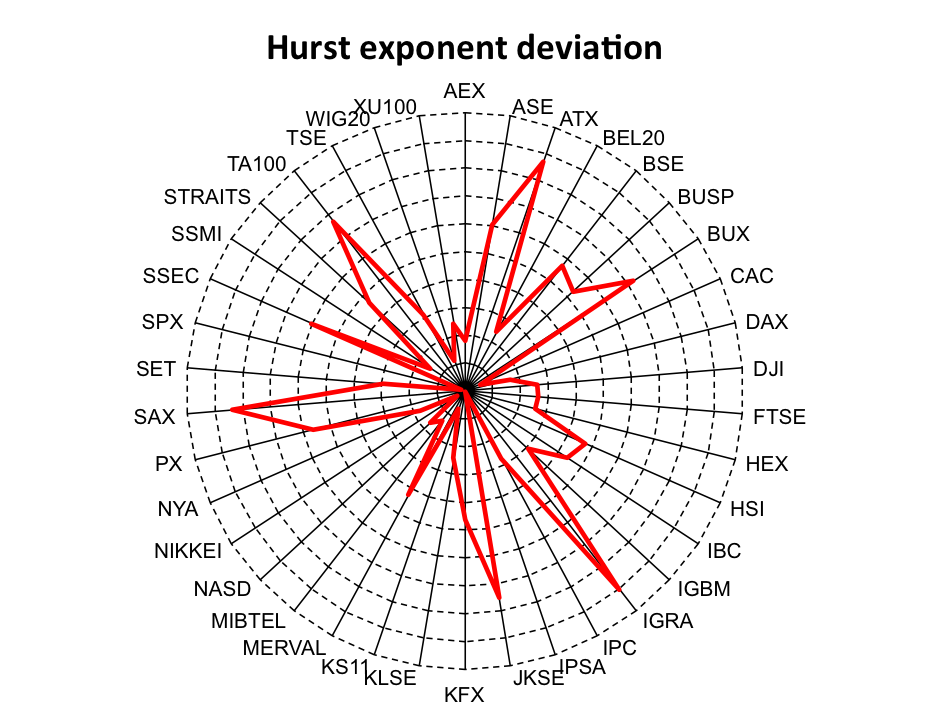
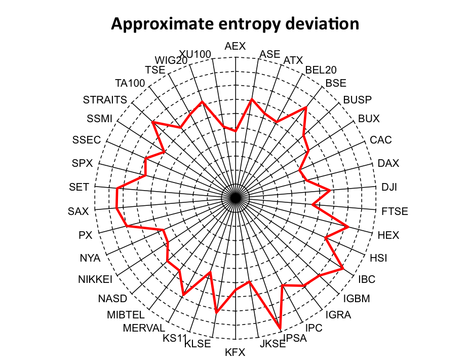
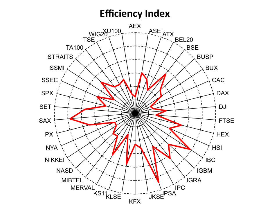
Figure 1: Hurst exponent, fractal dimension, approximate entropy and efficiency index for analyzed indices. The centers of the circle represent no deviation from the efficient market both for the specific deviations and for the Efficiency Index. The further the red line is from the center, the higher the deviation. The figures are rescaled to make the results more evident. From the Efficiency Index, we find that the Slovakian SAX, Venezuelan IBC, and Chilean IPSA are the least efficient markets whereas the Dutch AEX, French CAC and German DAX are the most efficient ones.

Table 1: List of the analyzed indices

Ticker	Index	Country
AEX	Amsterdam Exchange Index	Netherlands
ASE	Athens Stock Exchange General Index	Greece
ATX	Austrian Traded Index	Austria
BEL20	Euronext Brussels Index	Belgium
BSE	Bombay Stock Exchange Index	India
BUSP	Bovespa Brasil Sao Paulo Stock Exchange Index	Brasil
BUX	Budapest Stock Exchange Index	Hungary
CAC	Euronext Paris Bourse Index	France
DAX	Deutscher Aktien Index	Germany
DJI	Dow Jones Industrial Average Index	USA
FTSE	Financial Times Stock Exchange 100 Index	UK
HEX	OMX Helsinki Index	Finland
HSI	Hang Seng Index	Hong-Kong
IBC	Caracas Stock Exchange Index	Venezuela
IGBM	Madrid Stock Exchange General Index	Spain
IGRA	Peru Stock Market Index	Peru
IPC	Indice de Precios y Cotizaciones	Mexico
IPSA	Santiago Stock Exchange Index	Chile
JKSE	Jakarta Composite Index	Indonesia
KFX	Copenhagen Stock Exchange Index	Denmark
KLSE	Bursa Malaysia Index	Malaysia
KS11	KOSPI Composite Index	South Korea
MERVAL	Mercado de Valores Index	Argentina
MIBTEL	Borsa Italiana Index	Italy
NASD	NASDAQ Composite Index	USA
NIKKEI	NIKKEI 225 Index	Japan
NYA	NYSE Composite Index	USA
PX	Prague Stock Exchange Index	Czech Republic
SAX	Slovakia Stock Exchange Index	Slovakia
SET	Stock Exchange of Thailand Index	Thailand
SPX	Standard & Poor’s 500 Index	USA
SSEC	Shanghai Composite Index	China
SSMI	Swiss Market Index	Switzerland
STRAITS	Straits Times Index	Singapore
TA100	Tel Aviv 100 Index	Israel
TSE	Toronto Stock Exchange TSE 300 Index	Canada
WIG20	Warsaw Stock Exchange WIG 20 Index	Poland
XU100	Instanbul Stock Exchange National 100 Index	Turkey

Table 2: Descriptive statistics for the analyzed indices

Index	mean	min	max	SD	skewness	ex. kurtosis	KPSS	p-value
AEX	-0.0003	-0.0959	0.1003	0.0157	-0.0183	6.1531	0.1084	$>0.05$
ASE	-0.0006	-0.1021	0.1343	0.0169	-0.0697	5.0812	0.3531	$>0.05$
ATX	0.0002	-0.1025	0.1202	0.0150	-0.3410	8.2241	0.3141	$>0.05$
BEL20	-0.0001	-0.0832	0.0933	0.0135	0.0694	6.7098	0.1381	$>0.05$
BSE	0.0004	-0.1181	0.1599	0.0170	-0.1630	6.2487	0.1900	$>0.05$
BUSP	0.0004	-0.1210	0.1368	0.0193	-0.0641	4.5410	0.1229	$>0.05$
BUX	0.0004	-0.1265	0.1318	0.0169	-0.1105	6.3117	0.2860	$>0.05$
CAC	-0.0002	-0.0947	0.1060	0.0154	0.0594	5.3189	0.0944	$>0.05$
DAX	-0.0001	-0.0887	0.1080	0.0159	0.0025	4.7729	0.1681	$>0.05$
DJI	0.0000	-0.0820	0.1051	0.0126	-0.0089	7.8817	0.0647	$>0.05$
FTSE	-0.0001	-0.0927	0.0938	0.0129	-0.1309	6.4856	0.1222	$>0.05$
HEX	-0.0003	-0.1441	0.1344	0.0193	-0.1933	5.2159	0.1886	$>0.05$
HIS	0.0001	-0.1770	0.1341	0.0166	-0.2283	12.5630	0.1306	$>0.05$
IBC	0.0008	-0.2066	0.1453	0.0155	-0.4151	25.8530	0.2665	$>0.05$
IGBM	-0.0001	-0.1875	0.1840	0.0153	0.0833	20.5300	0.1272	$>0.05$
IGRA	0.0008	-0.1144	0.1282	0.0147	-0.3550	10.3010	0.3896	$>0.05$
IPC	0.0005	-0.0727	0.1044	0.0144	0.0515	4.3402	0.1295	$>0.05$
IPSA	0.0007	-0.0717	0.1180	0.0108	-0.0140	10.7400	0.1663	$>0.05$
JKSE	0.0006	-0.1095	0.0762	0.0150	-0.6570	6.1905	0.3397	$>0.05$
KFX	0.0002	-0.1172	0.0950	0.0137	-0.2594	5.7183	0.0939	$>0.05$
KLSE	0.0002	-0.1122	0.0537	0.0092	-1.1810	15.4970	0.1591	$>0.05$
KS11	0.0002	-0.1212	0.1128	0.0174	-0.4309	4.5849	0.1617	$>0.05$
MERVAL	0.0006	-0.1295	0.1612	0.0214	-0.1235	5.6617	0.1006	$>0.05$
MIBTEL	0.0002	-0.0771	0.0683	0.0108	-0.3979	5.7820	0.4301	$>0.05$
NASD	-0.0002	-0.1029	0.1116	0.0175	-0.1624	3.9587	0.2958	$>0.05$
NIKKEI	-0.0003	-0.1211	0.1324	0.0158	-0.3633	7.3242	0.1252	$>0.05$
NYA	0.0002	-0.1023	0.1153	0.0140	-0.4233	10.5210	0.1514	$>0.05$
PX50	0.0003	-0.1619	0.1236	0.0154	-0.6011	15.4230	0.4121	$>0.05$
SAX	0.0007	-0.0882	0.0711	0.0120	-0.0481	6.5294	0.5215	$>0.05$
SET	0.0000	-0.2211	0.1058	0.0158	-1.8111	26.2170	0.2975	$>0.05$
SPX	-0.0001	-0.0947	0.1096	0.0134	-0.1842	8.1808	0.0958	$>0.05$
SSEC	0.0002	-0.1200	0.0903	0.0168	-0.2784	4.7064	0.1461	$>0.05$
SSMI	-0.0001	-0.0811	0.1079	0.0127	0.0331	6.2488	0.0918	$>0.05$
STRAITS	0.0000	-0.2685	0.1406	0.0137	-2.2597	56.9590	0.1989	$>0.05$
TA100	0.0003	-0.0734	0.0978	0.0141	-0.1535	3.2977	0.1157	$>0.05$
TSE	0.0001	-0.0979	0.0937	0.0122	-0.6630	8.9915	0.0782	$>0.05$
WIG20	0.0004	-0.0886	0.3322	0.0185	2.6452	52.0680	0.1909	$>0.05$
XU100	0.0004	-0.1334	0.1749	0.0230	0.0039	4.5896	0.1105	$>0.05$

Table 3: Ranked stock indices according to the Efficiency Index

Index	Country	Hurst exponent	Fractal dimension	Approximate entropy	Efficiency index
AEX	Netherlands	0.5358	1.4356	0.5246	0.0619
CAC	France	0.5118	1.4592	0.5059	0.0628
DAX	Germany	0.5334	1.4646	0.4807	0.0698
XU100	Turkey	0.5493	1.4350	0.4870	0.0724
FTSE	UK	0.4470	1.5171	0.4500	0.0787
NYA	USA	0.5348	1.4457	0.4418	0.0821
NIKKEI	Japan	0.5063	1.4716	0.4285	0.0825
KS11	South Korea	0.5137	1.4204	0.4473	0.0829
SSMI	Switzerland	0.5297	1.4617	0.3983	0.0929
BEL20	Belgium	0.5481	1.4574	0.3869	0.0981
MIBTEL	Italy	0.5267	1.4728	0.3525	0.1063
NASD	USA	0.5340	1.4526	0.3428	0.1114
SPX	USA	0.5026	1.4437	0.3405	0.1119
KFX	Denmark	0.5927	1.4665	0.3516	0.1148
DJI	USA	0.4477	1.4685	0.3284	0.1165
BUX	Hungary	0.6448	1.4844	0.3811	0.1170
TSE	Canada	0.5626	1.4375	0.3272	0.1210
TA100	Israel	0.6536	1.4739	0.3648	0.1251
BUSP	Brazil	0.6055	1.4142	0.3435	0.1262
JKSE	Indonesia	0.6505	1.3657	0.3986	0.1311
WIG20	Poland	0.5232	1.4545	0.2790	0.1326
ATX	Austria	0.6744	1.4455	0.3669	0.1336
HSI	Hong-Kong	0.5945	1.4033	0.3033	0.1396
IPC	Mexico	0.5550	1.3817	0.2991	0.1398
ASE	Greece	0.6210	1.3926	0.2911	0.1518
SSEC	China	0.6205	1.3698	0.3019	0.1533
IGBM	Spain	0.5615	1.4581	0.1912	0.1691
STRAITS	Singapore	0.5937	1.4500	0.2027	0.1702
PX	Czech Rep	0.6124	1.4386	0.2053	0.1743
MERVAL	Argentina	0.5850	1.3729	0.2225	0.1745
HEX	Finland	0.5524	1.4385	0.1747	0.1768
BSE	India	0.6139	1.4313	0.1842	0.1841
SET	Thailand	0.5591	1.4311	0.1590	0.1851
KLSE	Malaysia	0.5489	1.3620	0.1773	0.1906
IGRA	Peru	0.6806	1.3435	0.2160	0.2108
SAX	Slovakia	0.6673	1.3132	0.1534	0.2421
IBC	Venezuela	0.5881	1.3308	0.0890	0.2439
IPSA	Chile	0.4997	1.3187	0.0239	0.2711

Table 4: Ranking of the indices according to the components

Index	Country	Efficiency Index	Hurst exponent	Fractal dimension	Approximate entropy
AEX	Netherlands	1	12	22	1
CAC	France	2	4	10	2
DAX	Germany	3	9	8	4
XU100	Turkey	4	15	23	3
FTSE	UK	5	18	2	5
NYA	USA	6	11	16	7
NIKKEI	Japan	7	3	5	8
KS11	South Korea	8	5	26	6
SSMI	Switzerland	9	8	9	10
BEL20	Belgium	10	13	12	11
MIBTEL	Italy	11	7	4	15
NASD	USA	12	10	14	18
SPX	USA	13	2	18	19
KFX	Denmark	14	25	7	16
DJI	USA	15	16	6	20
BUX	Hungary	16	33	1	12
TSE	Canada	17	22	21	21
TA100	Israel	18	35	3	14
BUSP	Brazil	19	28	27	17
JKSE	Indonesia	20	34	33	9
WIG20	Poland	21	6	13	26
ATX	Austria	22	37	17	13
HSI	Hong-Kong	23	27	28	22
IPC	Mexico	24	19	30	24
ASE	Greece	25	32	29	25
SSEC	China	26	31	32	23
IGBM	Spain	27	21	11	31
STRAITS	Singapore	28	26	15	30
PX	Czech Rep	29	29	19	29
MERVAL	Argentina	30	23	31	27
HEX	Finland	31	17	20	34
BSE	India	32	30	24	32
SET	Thailand	33	20	25	35
KLSE	Malaysia	34	14	34	33
IGRA	Peru	35	38	35	28
SAX	Slovakia	36	36	38	36
IBC	Venezuela	37	24	36	37
IPSA	Chile	38	1	37	38

References

- [1] J. Barunik, T. Aste, T. Di Matteo, and R. Liu. Understanding the source of multifractality in financial markets. Physica A, 391:4234–4251, 2012.
- [2] J. Barunik and L. Kristoufek. On Hurst exponent estimation under heavy-tailed distributions. Physica A, 389(18):3844–3855, 2010.
- [3] J. Beran. Statistics for Long-Memory Processes, volume 61 of Monographs on Statistics and Applied Probability. Chapman and Hall, New York, 1994.
- [4] D. Cajueiro and B. Tabak. Evidence of long range dependence in Asian equity markets: the role of liquidity and market restrictions. Physica A, 342:656–664, 2004.
- [5] D. Cajueiro and B. Tabak. The Hurst exponent over time: testing the assertion that emerging markets are becoming more efficient. Physica A, 336:521–537, 2004.
- [6] D. Cajueiro and B. Tabak. Ranking efficiency for emerging markets. Chaos, Solitons and Fractals, 22:349–352, 2004.
- [7] D. Cajueiro and B. Tabak. Ranking efficiency for emerging equity markets II. Chaos, Solitons and Fractals, 23:671–675, 2005.
- [8] R. Cont. Empirical properties of asset returns: stylized facts and statistical issues. Quantitative Finance, 1(2):223 – 236, 2001.
- [9] M. Couillard and M. Davison. A comment on measuring the hurst exponent of financial time series. Physica A, 348:404–418, 2005.
- [10] S. Davies and P. Hall. Fractal analysis of surface roughness by using spatial data. Journal of the Royal Statistical Society Series B, 61:3–37, 1999.
- [11] T. Di Matteo. Multi-scaling in finance. Quantitatice Finance, 7(1):21–36, 2007.
- [12] T. Di Matteo, T. Aste, and M. Dacorogna. Scaling behaviors in differently developed markets. Physica A, 324:183–188, 2003.
- [13] T. Di Matteo, T. Aste, and M. Dacorogna. Long-term memories of developed and emerging markets: Using the scaling analysis to characterize their stage of development. Journal of Banking & Finance, 29:827–851, 2005.
- [14] E. Fama. The behavior of stock market prices. Journal of Business, 38:34–105, 1965.
- [15] E. Fama. Efficient Capital Markets: A Review of Theory and Empirical Work. Journal of Finance, 25:383–417, 1970.
- [16] M.G. Genton. Highly robust variogram estimation. Mathematical Geology, 30:213–221, 1998.
- [17] J. Geweke and S. Porter-Hudak. The estimation and application of long memory time series models. Journal of Time Series Analysis, 4(4):221–238, 1983.
- [18] T. Gneiting and M. Schlather. Stochastic Models That Separate Fractal Dimension and the Hurst Effect. SIAM Review, 46(2):269–282, 2004.
- [19] T. Gneiting, H. Sevcikova, and D.B. Percival. Estimators of fractal dimension: Assessing the roughness of time series and spatial data. Technical report, Department of Statistics, University of Washington, 2010.
- [20] P. Hall and A. Wood. On the performane of box-counting estimators of fractal dimension. Biometrika, 80(1):246–252, 1993.
- [21] L. Kristoufek. Rescaled range analysis and detrended fluctuation analysis: Finite sample properties and confidence intervals. AUCO Czech Economic Review, 4:236–250, 2010.
- [22] L. Kristoufek. How are rescaled range analyses affected by different memory and distributional properties? A Monte Carlo study. Physica A, 391:4252–4260, 2012.
- [23] L. Kristoufek and M. Vosvrda. Capital markets efficiency: Fractal dimension, Hurst exponent and entropy (in Czech). Politická ekonomie, 16(2):208–221, 2012.
- [24] L. Kristoufek and M. Vosvrda. Measuring capital market efficiency: Global and local correlations structure. Physica A, 392:184–193, 2013.
- [25] L. Kristoufek and M. Vosvrda. Commodity futures and market efficiency. Energy Economics, 42:50–57, 2014.
- [26] H.R. Künsch. Statistical aspects of self-similar processes. Proceedings of the First World Congress of the Bernoulli Society, 1:67–74, 1987.
- [27] S. Lennartz and A. Bunde. Eliminating finite-size effects and detecting the amount of white noise in short records with long-term memory. Physical Review E, 79:066101, 2009.
- [28] K.-P. Lim. Ranking market efficiency for stock markets: A nonlinear perspective. Physica A, 376:445–454, 2007.
- [29] R. Morales, T. Di Matteo, and T. Aste. Non-stationary multifractality in stock returns. Physica A, 392:6470–6483, 2013.
- [30] R. Morales, T. Di Matteo, R. Gramatica, and T. Aste. Dynamical generalized Hurst exponent as a tool to monitor unstable periods in financial series. Physica A, 391:3180–3189, 2012.
- [31] S. Pincus. Approximate entropy as a measure of system complexity. PNAS, 88:2297–2301, 1991.
- [32] S. Pincus and R.E. Kalman. Irregularity, volatility, risk, and financial market time series. PNAS, 101(38):13709–13714, 2004.
- [33] P.M. Robinson. Gaussian semiparametric estimation of long range dependence. The Annals of Statistics, 23(5):1630–1661, 1995.
- [34] P. Samuelson. Proof that properly anticipated prices fluctuate randomly. Industrial Management Review, 6:41–49, 1965.
- [35] M. Taqqu, W. Teverosky, and W. Willinger. Estimators for long-range dependence: an empirical study. Fractals, 3(4):785–798, 1995.
- [36] M. Taqqu and V. Teverovsky. On Estimating the Intensity of Long-Range Dependence in Finite and Infinite Variance Time Series. In A Practical Guide To Heavy Tails: Statistical Techniques and Applications, 1996.
- [37] V. Teverovsky, M. Taqqu, and W. Willinger. A critical look at lo’s modified r/s statistic. Journal of Statistical Planning and Inference, 80(1-2):211–227, 1999.
- [38] R. Weron. Estimating long-range dependence: finite sample properties and confidence intervals. Physica A, 312:285––299, 2002.
- [39] W.-X. Zhou. Finite-size effect and the components of multifractality in financial volatility. Chaos, Solitons and Fractals, 45:147–155, 2012.
- [40] Z. Zhu and M. Stein. Parameter estimation for fractional brownian surfaces. Statistica Sinica, 12:863–883, 2002.
- [41] L. Zunino, M. Zanin, B. Tabak, D. Pérez, and O. Rosso. Complexity-entropy causality plane: A useful approach to quantify the stock market inefficiency. Physica A, 389:1891–1901, 2010.