Electrical detection of topological quantum phase transitions in disordered Majorana nanowires

Abstract

We study a disordered superconducting nanowire, with broken time-reversal and spin-rotational symmetry, which can be driven into a topological phase with end Majorana bound states by an externally applied magnetic field. It is known that as a function of disorder strength the Majorana nanowire has a delocalization quantum phase transition from a topologically non-trivial phase, which supports Majorana bound states, to a non-topological insulating phase without them. On both sides of the transition, the system is localized at zero energy albeit with very different topological properties. We propose an electrical transport measurement to detect the localization-delocalization transition occurring in the bulk of the nanowire. The basic idea consists of measuring the difference of conductance at one end of the wire obtained at different values of the coupling to the opposite lead. We show that this measurement reveals the non-local correlations emergent only at the topological transition. Hence, while the proposed experiment does not directly probe the end Majorana bound states, it can provide direct evidence for the bulk topological quantum phase transition itself.

Introduction. The study of topological phases of matter is one of the most active research topics in all of physics Nayak et al. (2008). A recent proposal to realize a one-dimensional (1D) topological superconductor (SC) Kitaev (2001) supporting zero-energy Majorana bound states (MBSs) in semiconductor-superconductor heterostructures Lutchyn et al. (2010); Oreg et al. (2010) has attracted great deal of attention, and has been explored experimentally Mourik et al. (2012); Das et al. (2012); Deng et al. (2012); Rokhinson et al. (2012); Finck et al. (2013); Churchill et al. (2013). However, despite this excitement, the issue remains largely open and the need of more decisive (i.e., “smoking gun”) evidence for the MBS scenario has been emphasized in recent works Pikulin et al. (2012); Bagrets and Altland (2012); Kells et al. (2012); Rieder et al. (2012); Motrunich et al. (2001); Liu et al. (2012); Das Sarma et al. (2012); Sau and Sarma (2013); Appelbaum (2013). In particular, no direct evidence for a topological quantum phase transition (TQPT), which is characterized by the closing of the superconducting gap and should accompany the emergence of MBSs, has been detected so far.

Disorder (e.g., impurities in the semiconductor) is an important relevant perturbation in the Majorana experiments Pikulin et al. (2012); Bagrets and Altland (2012); Liu et al. (2012); Sau and Sarma (2013); Lobos et al. (2012); Rainis et al. (2013), since the system is effectively a spinless p-wave superconductor with no Anderson theoremde Gennes (1966). Disorder and localization effects in superconductors with broken time-reversal and spin-rotational symmetries [i.e., symmetry class $D$ (Ref. Altland and Zirnbauer, 1997)] have been a subject of intense theoretical study Motrunich et al. (2001); Brouwer et al. (2000); Gruzberg et al. (2005); Brouwer et al. (2011a, b). In the work by Motrunich et al., it was shown that disorder-induced subgap Andreev bound states proliferate in a class $D$ superconductor near zero energy, and therefore a closing of the bulk SC gap at the TQPT is an ill-defined concept since gap closing has no meaning if the system is already gapless.Motrunich et al. (2001). Nevertheless, the system still has well-defined topological properties and generically lies in one of two topologically distinct phases. For weak disorder, an infinite system is in a non-trivial topological phase characterized by the presence of two degenerate zero-energy MBSs localized at the ends of the wire. In a finite-length system of size $L$, this degeneracy is lifted by an exponential splitting $\sim e^{-L/\xi}$, where $\xi$ is the superconducting coherence length. Increasing the strength of disorder induces a proliferation of low-energy Andreev bound states (i.e., quantum Griffiths effect), and the splitting scales as $\sim e^{L/\xi+L/(2\ell_{e})}$, where $\ell_{e}$ is the elastic mean-free path of the system.Brouwer et al. (2011a) Beyond a critical disorder strength (defined by the condition $\ell_{e}=\xi/2$), the system enters a nontopological insulating phase with no end-MBSs. At both sides of the TQPT, the system is localized at zero energy, and exactly at the critical point separating these phases, the wave functions become delocalized and the smallest Lyapunov exponent (i.e., the inverse of the localization length of the system) vanishes. This key observation links the physics of localization and topological properties of a disordered $D$-class SC wire Akhmerov et al. (2011); DeGottardi et al. (2011, 2013); Sau and Das Sarma (2012); Adagideli et al. (2013). For example, it has been shown that the quantity $Q=\text{sign }\left(\text{Det }r\right)=\text{sign}(\prod_{n=1}^{2M}\tanh\lambda_{n})$, where $r$ is the reflection matrix and $\lambda_{n}$ is the Lyapunov exponent related to the $n$-th transmission channel, is a suitable topological invariant for a disordered class $D$ superconductor, which changes sign whenever a Lyapunov exponent crosses zero Akhmerov et al. (2011); Fulga et al. (2011). It was suggested that the delocalized nature of the wave functions, with their non-local correlations that appear at the topological critical point, could be observed in the quantization of the thermal conductance $G_{\text{th}}/G_{0}=1$ (with $G_{0}=\pi^{2}k_{B}^{2}T/6h$ at temperature $T$) or the onset of quantized non-local current-noise correlations, constituting evidence for the TQPT. Unfortunately, the highly challenging requirements of these experiments have hindered further progress.

In this work we propose a different yet simple, electrical transport experiment to detect the TQPT, measuring directly the non-local correlations in the bulk appearing exactly at the critical point. We study a disordered topological SC coupled to left and right normal leads in a normal-superconducting-normal (NSN) device as depicted in Fig. 1. Instead of computing the left-right conductance $G_{LR}$, our proposal consists in calculating the local conductance at one end of the NW, while tuning the coupling to the opposite lead. As we show below, this procedure allows to extract information about the non-local correlations, which in turn could be used to identify the TQPT in the bulk of the wire. We stress that this is different from measuring $G_{LR}$ , which vanishes, or from measuring the non-local correlations in the shot noise Bolech and Demler (2007). Our method can be immediately implemented in on-going experiments looking for zero bias conductance peak in the Majorana nanowires.

Theoretical model. We firstmotivate our results by studying a 1D solvable model of a disordered $D$-class SC consisting of spinless Dirac fermions with a random $p$-wave gap $\Delta(x)$. In the Majorana basis the Hamiltonian, from $x=0$ to $x=L$, is Brouwer et al. (2011a); Akhmerov et al. (2011) $H_{\text{w}}=-i\hbar v_{F}\sigma^{z}\partial_{x}+\sigma^{y}\Delta(x)$, where $(\sigma^{x},\sigma^{y},\sigma^{z})$ is the vector of Pauli matrices acting on the space of right- and left-moving Majorana fields. At zero energy, this Hamiltonian has localized Majorana modes at the ends of the wire, e.g., $\Psi(x)=\exp[-(1/\hbar v_{F})\int_{0}^{x}dx^{\prime}\ \Delta\left(x^{\prime}\right)\sigma^{x}]\Psi\left(0\right)$ is a localized mode at the left end (i.e., $x=0$). The reflection $r_{1}=\tanh(L\bar{\Delta}/\hbar v_{F})$ and transmission $t_{1}=\cosh^{-1}(L\bar{\Delta}/\hbar v_{F})$ amplitudes are obtained by imposing $\Psi(0)=(1,r_{1})^{T}$, $\Psi(L)=(t_{1},0)^{T}$ where $\bar{\Delta}=L^{-1}\int_{0}^{L}dx\ \Delta\left(x\right)$ is the average $p$-wave gap. Assuming that $\bar{\Delta}$ can be controlled with an external tuning parameter (e.g., external magnetic field), the TQPT in this model occurs when $\bar{\Delta}=0$, and is accompanied by a change of sign in $r_{1}$ (which can be interpreted as the topological invariant), and by a peak in the thermal conductance $G_{\text{th}}/G_{0}=\text{Tr }t_{1}t_{1}^{*}=\cosh^{-2}(L\bar{\Delta}/\hbar v_{F})$, of width equal to the Thouless energy of the system, i.e., $\hbar v_{F}/L$. This result is a consequence of the particular reflection-less boundary condition imposed at the right end of the wire, $x=L$. However, one can assume a more general situation introducing a barrier at the end of the wire, described by a generic scatterer with reflection and transmission amplitudes $r_{2}$ and $t_{2}$, respectively (subject to the unitarity constraint $\left|r_{2}\right|^{2}+\left|t_{2}\right|^{2}=1$). This would correspond to an imperfect coupling to the right lead or to any backscatterer which is external to the wire itself. The total reflection amplitude becomes

$$r =r_{1}+t_{1}\left(\frac{r_{2}}{1+r_{2}r_{1}}\right)t_{1}.$$ (1)

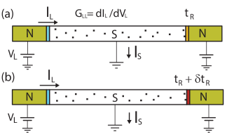
Figure 1: (Color online) Schematic representation of the N-S-N system under consideration. The basic idea consists of measuring the conductance at one end of the NW (e.g. left end) for different values of $\gamma_{R}$, the coupling to the opposite (i.e., right) lead. The difference of conductances $\delta G_{LL}$ [see Eq. (9)] contains information about the non-local correlations between the end-points of the NW, which can be used to detect the TQPT.

Intuitively, the last term in Eq. (1) represents processes in which the right-moving Majorana mode is transmitted to the right end of the wire with amplitude $t_{1}$, and is reflected back with amplitude $r_{2}$ as a left-mover. This result means that the quantity $r$ in general contains non-local contributions from the scattering occurring at the right endBüttiker (1986). Note that for a non-vanishing $r_{2}$ the point $r=0$ is shifted with respect to the topological transition in the bulk of the wire $\bar{\Delta}=0$. This shift is of the order of the intrinsic width $\sim\hbar v_{F}/L$ of the TQPT, and hence does not affect its experimental detection. Let us now assume that $r_{2}$ is another external tunable parameter in the system, in which case a small variation $\delta r_{2}$ around $r_{2}=0$ allows to extract the non-local contributions in Eq. (1), i.e., $\delta r\approx\delta r_{2}\cosh^{-2}(L\bar{\Delta}/\hbar v_{F})$, which is non-vanishing only near the TQPT, indicating the delocalization of the Majorana wave function $\Psi\left(x\right)$. Since these properties depend only on the symmetry class of the Hamiltonian, we expect these findings to be model independent and to apply to all types class-$D$ Bogoliubov-de Gennes (BdG) Hamiltonians. This is the main idea of this work.

We now consider a more realistic model for a $D-$class superconducting wire consisting of a 1D semiconductor NW of length $L$ along the $x$ axis with a strong spin-orbit coupling (SOC), an external magnetic field along $x$, and proximity induced $s-$wave pairing due to a proximate bulk SC Lutchyn et al. (2010); Oreg et al. (2010). Discretizing the continuum system and assuming single subband occupancy, the effective low-energy model corresponds to an $N-$site tight-binding model $H=H_{\text{w}}+H_{\text{leads}}+H_{\text{mix}}$ Stanescu et al. (2011), with

$$H_{\text{w}}= -t\sum_{\langle lm\rangle,s}c_{l,s}^{\dagger}c_{m,s}-\sum_{l,s}c_{l,s}^{\dagger}\left(\mu_{l}-V_{Z}\sigma_{ss^{\prime}}^{x}\right)c_{l,s^{\prime}}$$

$$+\sum_{l,s}\left(i\alpha\ c_{l,s}^{\dagger}\sigma_{ss^{\prime}}^{y}c_{l+1,s^{\prime}}+\Delta_{0}c_{l\uparrow}^{\dagger}c_{l\downarrow}^{\dagger}+{\rm H.c.}\right),$$ (2)

with effective hopping parameter $t$ and lattice parameter $a$. Here $c_{l,s}^{\dagger}$ creates an electron with spin projection $s=\left\{\uparrow,\downarrow\right\}$ at site $l$ in the tight-binding chain, $\alpha$ is the Rashba SOC parameter, $V_{Z}$ is the Zeeman energy due to an external magnetic field along $x$, and $\Delta_{0}$ is the induced $s$-wave gap which must be calculated self-consistently. Since the precise numerical value of $\Delta_{0}$ does not modify our conclusions, here we make the simplifying assumption that $\Delta_{0}$ already satisfies the self-consistent SC gap equation.

Short-ranged nonmagnetic static disorder in the semiconductor NW is included through a fluctuating chemical potential $\mu_{l}=\mu_{0}+\delta\mu_{l}$ about the average $\mu_{0}$. For simplicity we assume $\delta\mu_{l}$ to be a delta-correlated random variable with Gaussian distribution, $\left\langle\delta\mu_{l}\delta\mu_{m}\right\rangle=v_{0}^{2}\delta_{lm}$. Hamiltonian in Eq. 2 is another particular example of a disordered $D-$class SC Altland and Zirnbauer (1997). As a function of the external Zeeman field $V_{Z}$, and in absence of disorder this model has a TQPT from a topologically trivial phase to non-trivial phase with end MBS at the value $V_{Z,c}=\sqrt{\mu_{0}^{2}+\Delta_{0}^{2}}$ as shown originally by Sau et al. Sau et al. (2010a). In the presence of disorder, the critical field $V_{Z,c}$ shifts to higher values, and its precise value depends on the particular details of the disorder Brouwer et al. (2011a, b); Adagideli et al. (2013).

We describe the coupling to the external leads (see Fig. 1), by the term $H_{\text{mix}}=\sum_{s}(t_{L}f_{Lk,s}^{\dagger}c_{1,s}+t_{R}f_{Rk,s}^{\dagger}c_{N,s})+\text{H.c.,}$ where $t_{L\left(R\right)}$ is the coupling to the left (right) lead and $f_{L\left(R\right)k,s}^{\dagger}$ is the corresponding creation operator for fermions with quantum number $k$ and spin $s$. The external leads are modeled as large Fermi liquids with Hamiltonian $H_{\text{lead},j}=\sum_{k,s}\epsilon_{k}f_{j,k,s}^{\dagger}f_{j,k,s}$, where $j=\{L,R\}$.

At $T=0$, the local and non-local zero-bias conductances have the explicit form Blonder et al. (1982); Anantram and Datta (1996) (see Appendix A)

$$G_{LL} = \frac{e^{2}}{h}\{M_{L}-\text{Tr }[r_{ee}r_{ee}^{\dagger}]+\text{Tr }[r_{eh}r_{eh}^{\dagger}]\},$$ (3)

$$G_{LR} = -\frac{e^{2}}{h}\{\text{Tr }[t_{ee}t_{ee}^{\dagger}]-\text{Tr }[t_{eh}t_{eh}^{\dagger}]\},$$ (4)

where $M_{L}=\sum_{\sigma}2\pi\gamma_{L}\rho_{1\sigma}(0)$ is the number of transmission channels at energy $\omega=0$ in the left lead. Here $\rho_{l\sigma}\left(\omega\right)$ is the local density of states at site $l$ in the chain, and $\gamma_{j}\equiv 2\pi t_{j}^{2}\rho_{j}^{0}$ is the broadening of levels due to the leakage to the lead $j$, described by the local density of states $\rho_{j}^{0}$ (assumed to be $SU(2)$-symmetric and constant around the Fermi energy). In addition, we have defined, respectively, the normal and Andreev reflection matrices at the left lead, i.e., $\left[r_{ee}\left(\omega\right)\right]_{s,s^{\prime}}\equiv\gamma_{L}g_{1s,1s^{\prime}}^{r}\left(\omega\right)$, $\left[r_{eh}\left(\omega\right)\right]_{s,s^{\prime}}\equiv\gamma_{L}f_{1s,1s^{\prime}}^{r}\left(\omega\right)$, and the normal and Andreev transmission matrices, i.e., $\left[t_{ee}\left(\omega\right)\right]_{s,s^{\prime}}\equiv\sqrt{\gamma_{L}\gamma_{R}}g_{1s,Ns^{\prime}}^{r}\left(\omega\right)$ and $\left[t_{eh}\left(\omega\right)\right]_{s,s^{\prime}}\equiv\sqrt{\gamma_{L}\gamma_{R}}f_{1s,Ns^{\prime}}^{r}\left(\omega\right)$, where $g_{ls,ms^{\prime}}^{r}\left(\omega\right)$ and $f_{ls,ms^{\prime}}^{r}\left(\omega\right)$ are the normal and anomalous retarded Green’s functions in the chain (see Appendix A).

The topological phase occurring for $V_{Z}>V_{Z,c}$ is characterized by a quantized zero-bias peak at $G_{LL}=2e^{2}/h$, which is a direct consequence of an MBS localized at the left end of the NW Law et al. (2009); Sau et al. (2010b); Flensberg (2010); Wimmer et al. (2011). However, the proliferation of disorder-induced subgap Andreev bound states near zero energy results in a power-law singularity $\left\langle\rho_{1,\sigma}\left(\omega\right)\right\rangle_{\text{dis}}\sim 1/\left|\omega\right|^{\nu}$ in the disorder-averaged density of states, and complicates the interpretation of this zero-bias peak Motrunich et al. (2001); Sau and Sarma (2013); Brouwer et al. (2000); Gruzberg et al. (2005); Brouwer et al. (2011a, b). On the other hand, the experimental detection of the predicted delocalization TQPT is hindered by the fact that the non-local electrical conductance $G_{LR}\left(0\right)$ vanishes, since $\text{Tr }[t_{ee}t_{ee}^{\dagger}]=\text{Tr }[t_{eh}t_{eh}^{\dagger}]$ at the transition Akhmerov et al. (2011). In addition, the predicted quantized thermal conductance $G_{\text{th}}/G_{0}=2\text{Tr }[t_{ee}t_{ee}^{\dagger}+t_{eh}t_{eh}^{\dagger}]$ is experimentally very difficult to observe. This calls for alternative methods to detect the TQPT.

In analogy to Eq. (1), Eq. (3), despite being a local quantity computed at the left lead, contains information about the non-local correlations in the NW. To see this, we make use of the Green’s function identityKadanoff and Baym (1989) $\boldsymbol{\mathcal{G}}^{r}\left(\omega\right)-\boldsymbol{\mathcal{G}}^{a}\left(\omega\right)=\boldsymbol{\mathcal{G}}^{r}\left(\omega\right)\left[\boldsymbol{\Sigma}^{r}\left(\omega\right)-\boldsymbol{\Sigma}^{a}\left(\omega\right)\right]\boldsymbol{\mathcal{G}}^{a}\left(\omega\right)$, where $\boldsymbol{\mathcal{G}}^{r\left(a\right)}\left(\omega\right)=[\omega-\boldsymbol{\mathcal{H}}_{\text{w}}^{\text{BdG}}-\boldsymbol{\Sigma}^{r\left(a\right)}]^{-1}$ is the Green’s function matrix, defined in terms of the $2\times 2$ Nambu blocks

$$\boldsymbol{\mathcal{G}}^{r\left(a\right)}\left(\omega\right)=\left(\begin{array}[]{cc}g^{r}\left(\omega\right)&f^{r}\left(\omega\right)\\ \bar{f}^{r}\left(\omega\right)&\bar{g}^{r}\left(\omega\right)\end{array}\right),$$ (7)

$\boldsymbol{\mathcal{H}}_{\text{w}}^{\text{BdG}}$ is the BdG Hamiltonian corresponding to Eq. (2), and $\boldsymbol{\Sigma}^{r\left(a\right)}\left(\omega\right)=\mp(i/2)\left(\gamma_{L}\delta_{l,1}+\gamma_{R}\delta_{l,N}\right)\delta_{s,s^{\prime}}$ is the retarded (advanced) self-energy due to the coupling $H_{\text{mix}}$. This allows us to express Eq. (3) in a more suggestive form

$$G_{LL} =\frac{e^{2}}{h}\{2\text{Tr }[r_{eh}r_{eh}^{\dagger}]+\text{Tr }[t_{ee}t_{ee}^{\dagger}+t_{eh}t_{eh}^{\dagger}]\},$$ (8)

which is reminiscent to Eq. (1), and where last term is the (dimensionless) thermal conductance $G_{\text{th}}/G_{0}$. This term vanishes in the limit $L~{}\to~{}\infty$, where we recover the usual expression $G_{LL}=(2e^{2}/h)\text{Tr}[r_{eh}r_{eh}^{\dagger}]$ found in the literature Law et al. (2009); Wimmer et al. (2011). Changing the coupling to the right lead, $\gamma_{R}\to\gamma_{R}+\delta\gamma_{R}$ (keeping all the other parameters fixed) amounts to varying the reflection amplitude $r_{2}$ in the continuum model, and hence we expect to obtain non-local correlations at the TQPT. Experimentally, $\gamma_{R}$ and $\gamma_{L}$ could be easily modified varying the pinch-off gates underneath the ends of the NW, constituting a useful experimental knob in the Majorana experiment, which has not been exploited in Refs. Mourik et al. (2012); Das et al. (2012); Deng et al. (2012); Rokhinson et al. (2012); Finck et al. (2013); Churchill et al. (2013). In particular, one can easily show that the change in $G_{LL}$ at zero bias,

$$\delta G_{LL} \equiv G_{LL}\left(\gamma_{R}+\delta\gamma_{R},\gamma_{L}\right)-G_{LL}\left(\gamma_{R},\gamma_{L}\right),$$ (9)

is a purely non-local contribution proportional to $\boldsymbol{\mathcal{G}}_{1\sigma,N\sigma^{\prime}}^{r\left(a\right)}\left(\omega\right)$, $\boldsymbol{\mathcal{G}}_{N\sigma,1\sigma^{\prime}}^{r\left(a\right)}\left(\omega\right)$ and $\boldsymbol{\mathcal{G}}_{N\sigma,N\sigma^{\prime}}^{r\left(a\right)}\left(\omega\right)$ (see appendix A for details). In agreement with our previous results, this contribution will be only non-vanishing when the single-particle wave functions become delocalized, allowing a simple electrical detection of the TQPT.

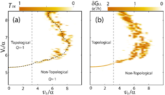
Figure 2: (Color online). (a) Transmission probability $T_{1N}$ between the end-points (sites $1$ and $N$) of the isolated NW and topological phase diagram as a function of disorder strength $v_{0}$ and Zeeman field $V_{Z}$. At the topological critical point, the topological invariant $Q=\text{sign}(\prod_{n=1}^{4}\tanh\lambda_{n})$, where $\lambda_{n}$ are the Lyapunov exponents, changes sign and the transmission probability $T_{1N}$ becomes 1 [see also Fig. 3(a)]. The bold dashed line follows the TQPT. (b) Difference of left conductances $\delta G_{LL}$ [see Eq. (9)]. We have chosen parameters $\gamma_{L}=0.2t$, $\gamma_{R}=10^{-5}t$, $\delta\gamma_{R}=10^{-3}t$, $N=300$, $\alpha=0.07t$, $\Delta=0.37t$ and $\mu_{0}=-2t$. In the clean case and at $V_{z}=0.45t=6.4\alpha$ we obtain the maximal ratio of $L/\xi\sim 10$ where $L$ is the length of the NW.

Transfer matrix. We consider a single disorder realization $\boldsymbol{\delta\mu}=\{\delta\mu_{1},\dots,\delta\mu_{N}\}$, and vary an overall prefactor, the disorder strength $v_{0}$. Presumably, a fixed disorder realization is closer to the experiments, where the semiconductor NW is in the mesoscopic regime, and it is not clear that disorder necessarily self-averages at the very low experimental temperatures. We have computed the topological phase diagram using the transfer matrix methodDeGottardi et al. (2011) for an isolated NW using the model Hamiltonian of Eq. (2) The transfer matrix for zero-energy modes is given by $M=\prod_{l=1}^{N}M_{l}$, where (see Appendix  B)

$$M_{l} = \left(\begin{array}[]{cccc}\frac{-t\mu_{l}+\alpha(V_{z}-\Delta_{0})}{t^{2}+\alpha^{2}}&\frac{-\alpha\mu_{l}+t(V_{z}+\Delta_{0})}{t^{2}+\alpha^{2}}&\frac{t}{t^{2}+\alpha^{2}}&\frac{\alpha}{t^{2}+\alpha^{2}}\\ \frac{\alpha\mu_{l}+t(V_{z}-\Delta_{0})}{t^{2}+\alpha^{2}}&\frac{-t\mu_{l}-\alpha(V_{z}+\Delta_{0})}{t^{2}+\alpha^{2}}&\frac{-\alpha}{t^{2}+\alpha^{2}}&\frac{t}{t^{2}+\alpha^{2}}\\ -t&-\alpha&0&0\\ \alpha&-t&0&0\end{array}\right).$$

The eigenvalues of $M$ are denoted by $e^{\pm\lambda_{n}}$, where the Lyapunov exponent $\lambda_{n}$ is related to the transmission probability by $T_{1N}=\sum_{n=1}^{4}T_{n}$, with $T_{n}=1/\cosh^{2}\lambda_{n}$ the transmission eigenvalue corresponding to the $n-$th channel. At the TQPT one of the Lyapunov exponents in the NW vanishes and, consequently, the corresponding transmission eigenvalue becomes $T_{n}=1$, while the topological invariant $Q$ changes sign.

Disscussion. In Fig. 2(a) we show the topological quantum phase diagram in the Zeeman field vs disorder strength plane. Fig. 2(b) shows the $\delta G_{LL}$ conductance map for exactly the same parameters as in Fig. 2a. Although $\delta G_{LL}$ is computed for an open system, while $T_{1N}$ has been computed for the isolated wire ($\gamma_{L}=\gamma_{R}=0$), the remarkable agreement between Fig. 2(a) and 2(b) is encouraging for the experimental detection of the TQPT using $\delta G_{LL}$.

In Fig. 3(a) and 3(b) we compare the transmission probability $T_{1N}$ and the topological invariant $Q$ for the isolated NW for a particular disorder strength with $\delta G_{LL}$ in the limit $\delta\gamma_{R}\ll\gamma_{R}=\gamma_{L}=1.4\alpha$, for various $\delta\gamma_{R}$. As we see, these two quantities follow each other closely. While the width of the peaks is the same in all cases (as expected, since the Thouless energy $\hbar v_{F}/L$ is an intrinsic property of $H_{\text{w}}$), the maximum of $\delta G_{LL}$ is shifted with respect to the maximum of $T_{1N}$, indicative of some reflection occurring at the NS barriers.

In practice, our proposal is expected to work best for short wires, where the maximal ratio $L/\xi$ is not too large. Note that the visibility of the electrical signal crucially depends on the width $~{}\hbar v_{F}/L$ of the peak in $\delta G_{LL}$. A very narrow peak might be hard to detect, or could be washed away by finite temperature effects or other dissipative mechanisms not taken into consideration here. Also, the system should be smaller than the phase-relaxation length $L<L_{\phi}$. Despite these limitations, our predictions are within experimental reachMourik et al. (2012); Das et al. (2012); Deng et al. (2012); Rokhinson et al. (2012); Finck et al. (2013); Churchill et al. (2013) since we obtain $\xi\approx 20$ nm with the experimental value of $L\approx 2$ $\mu$m. Similarly, the width of the peak in $\delta G_{LL}$, proportional to the Thouless energy, is of the order of $\hbar v_{F}/L\approx 52$ $\mu$eV, also within experimental resolution.

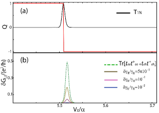
Figure 3: (Color online). (a) Topological invariant for an isolated NW. The localization -delocalization transition is evident form the appearance of a quantized peak in the transmission probability, $T_{1N}$. (b) difference in conductance in the left lead for different couplings to the right lead in the regime $\delta\gamma_{R}\ll\gamma_{R}$. The main point is that these two quantities follow each other which can be used to detect the topological phase transition. Here we have chosen fixed disorder amplitude $v_{0}=3.14\alpha$, see dashed vertical lines in Fig. 2.

In conclusion, we have developed a method to experimentally detect the topological phase transition in disordered class $D$ SC NWs, like those under investigation in Refs. Mourik et al. (2012); Das et al. (2012); Deng et al. (2012); Rokhinson et al. (2012); Finck et al. (2013); Churchill et al. (2013). While this method cannot provide direct evidence for MBS, it is can provide robust evidence of the topological phase transition itself in disordered NWs. The basic idea is to measure the differences of conductance at one end of the NW (e.g., the left end) for different values of the coupling with the opposite lead. We note that this procedure can be easily implemented in on-going experiments and provides a complementary technique of studying topological physics in Majorana-carrying systems by directly studying the bulk TQPT rather than the Majorana zero modes themselves.

The authors thank L. Arrachea for useful comments and acknowledge support from DARPA QuEST, NSF through the PFC@JQI, Conacyt, and Microsoft Q.

Appendix A Calculation of the conductance matrix in a SNS contact

Here we provide the details of the calculations of the conductance through a generic NSN system. Our derivation is standard and makes use of the so-called Hamiltonian formalism Cuevas et al. (1996), which is equivalent to the the more frequently-used scattering or BTK formalism Blonder et al. (1982); Anantram and Datta (1996), provided the Green functions are calculated to all orders in the coupling across the SN interface. Our model Hamiltonian in the main text is

$$H =H_{\text{w}}+H_{\text{mix}}+H_{\text{lead, L}}+H_{\text{lead, R}},$$ (11)

$$H_{\text{w}} =-t\sum_{\langle lm\rangle,s}c_{l,s}^{\dagger}c_{m,s}-\sum_{l,s}c_{l,s}^{\dagger}\left(\mu_{l}-V_{Z}\sigma_{ss^{\prime}}^{x}\right)c_{l,s^{\prime}}+\sum_{l,s}\left(i\alpha\ c_{l,s}^{\dagger}\sigma_{ss^{\prime}}^{y}c_{l+1,s^{\prime}}+\Delta_{0}c_{l\uparrow}^{\dagger}c_{l\downarrow}^{\dagger}+{\rm H.c.}\right),$$ (12)

$$H_{\text{mix}} =\sum_{s}(t_{L}f_{Lk,s}^{\dagger}c_{1,s}+t_{R}f_{Rk,s}^{\dagger}c_{N,s})+\text{H.c.,}$$ (13)

$$H_{\text{lead},j} =\sum_{k,s}\epsilon_{k}f_{j,k,s}^{\dagger}f_{j,k,s}.$$ (14)

We assume that each lead is in equilibrium at a chemical potential $\mu_{j}=eV_{j}$ controlled by external voltages, where $j=\left\{L,R\right\}$, and that the SC NW is grounded, i.e., $\mu_{S}=0$ (see Fig. 1). The expression for the electric current calculated through the contacts is $I_{j}=e\langle dN_{j}/dt\rangle=ie\langle[H,N_{j}]\rangle/\hbar=ie\langle[H_{\text{mix}},N_{j}]\rangle/\hbar$, which can be written in terms of the Green function at the contacts as Cuevas et al. (1996); Meir and Wingreen (1992)

$$I_{L} =\frac{ie}{\hbar}\sum_{\sigma}t_{L}\left[\left\langle c_{L,\sigma}^{\dagger}c_{1,\sigma}\right\rangle-\left\langle c_{1,\sigma}^{\dagger}c_{L,\sigma}\right\rangle\right],$$ (15)

$$I_{R} =\frac{ie}{\hbar}\sum_{\sigma}t_{L}\left[\left\langle c_{R,\sigma}^{\dagger}c_{N,\sigma}\right\rangle-\left\langle c_{N,\sigma}^{\dagger}c_{R,\sigma}\right\rangle\right].$$ (16)

With these definitions, note that the currents are positive if particles move into the leads (i.e., exit the SC), and negative otherwise. On the other hand, charge conservation demands that $I_{L}+I_{R}+I_{S}=0$, where $I_{S}$ is the excess current that flows to earth through the SC. Within the Baym-Kadanoff-Keldysh formalism Kadanoff and Baym (1989) we define the lesser Green function

$$g_{i\sigma,j\sigma^{\prime}}^{<}\left(t\right) \equiv ie\left\langle c_{i,\sigma}^{\dagger}c_{j,\sigma}\left(t\right)\right\rangle,$$ (17)

so that we can write the currents as

$$I_{L} =\frac{e}{\hbar}t_{L}\sum_{\sigma}\int_{-\infty}^{\infty}\frac{d\omega}{2\pi}\left[g_{L\sigma,1\sigma}^{<}\left(\omega\right)-g_{1\sigma,L\sigma}^{<}\left(\omega\right)\right],$$ (18)

$$I_{R} =\frac{e}{\hbar}t_{R}\sum_{\sigma}\int_{-\infty}^{\infty}\frac{d\omega}{2\pi}\left[g_{R\sigma,N\sigma}^{<}\left(\omega\right)-g_{N\sigma,R\sigma}^{<}\left(\omega\right)\right],$$ (19)

Using equations of motion, we can express Eqs. 18 and 19 in terms of local Green’s functions as Cuevas et al. (1996); Meir and Wingreen (1992)

$$I_{L} =-\frac{e}{h}t_{L}^{2}\sum_{\sigma}\int_{-\infty}^{\infty}d\omega\left[g_{L\sigma,L\sigma}^{0,<}\left(\omega\right)g_{1\sigma,1\sigma}^{>}\left(\omega\right)-g_{L\sigma,L\sigma}^{0,>}\left(\omega\right)g_{1\sigma,1\sigma}^{<}\left(\omega\right)\right],$$ (20)

$$I_{R} =-\frac{e}{h}t_{R}^{2}\sum_{\sigma}\int_{-\infty}^{\infty}d\omega\left[g_{R\sigma,R\sigma}^{0,<}\left(\omega\right)g_{N\sigma,N\sigma}^{>}\left(\omega\right)-g_{R\sigma,R\sigma}^{0,>}\left(\omega\right)g_{N\sigma,N\sigma}^{<}\left(\omega\right)\right].$$ (21)

Our first step to obtain the expression of the currents is to specify the unperturbed Green’s functions $g_{j\sigma,j\sigma}^{0,\gtrless}\left(\omega\right)$ in the leads, with $j=\left\{L,R\right\}$:

$$g_{j\sigma,j\sigma}^{0,<}\left(\omega\right) =2\pi i\rho_{j,\sigma}^{0}\left(\omega\right)n_{j}\left(\omega\right),$$

$$g_{j\sigma,j\sigma}^{0,>}\left(\omega\right) =2\pi i\rho_{j,\sigma}^{0}\left(\omega\right)\left[n_{j}\left(\omega\right)-1\right],$$

where $n_{j}\left(\omega\right)=n_{F}\left(\omega+\mu_{j}\right)$ are the Fermi distribution functions at the leads. Substituting these expressions gives

$$I_{L} =-\frac{ie}{h}2\pi t_{L}^{2}\sum_{\sigma}\int_{-\infty}^{\infty}d\omega\;\rho_{L,\sigma}^{0}\left(\omega\right)\left\{n_{L}\left(\omega\right)\left[g_{1\sigma,1\sigma}^{r}\left(\omega\right)-g_{1\sigma,1\sigma}^{a}\left(\omega\right)\right]+g_{1\sigma,1\sigma}^{<}\left(\omega\right)\right\},$$ (22)

$$I_{R} =-\frac{ie}{h}2\pi t_{R}^{2}\sum_{\sigma}\int_{-\infty}^{\infty}d\omega\;\rho_{R,\sigma}^{0}\left(\omega\right)\left\{n_{R}\left(\omega\right)\left[g_{N\sigma,N\sigma}^{r}\left(\omega\right)-g_{N\sigma,N\sigma}^{a}\left(\omega\right)\right]+g_{N\sigma,N\sigma}^{<}\left(\omega\right)\right\},$$ (23)

where we have used the identityKadanoff and Baym (1989); Mahan (1981) $g^{>}\left(\omega\right)-g^{<}\left(\omega\right)=g^{r}\left(\omega\right)-g^{a}\left(\omega\right)$. Obtaining an explicit expression for the currents $I_{L}$ and $I_{R}$ is quite cumbersome. Since we will be interested only in the conductance, we note that there is an enormous simplification if we compute directly the conductance matrix by deriving the currents with respect to the voltages $V_{L},V_{R}$. Then

$$G_{LL}\equiv\frac{dI_{L}}{dV_{L}} =-\frac{ie^{2}}{h}2\pi t_{L}^{2}\sum_{\sigma}\int_{-\infty}^{\infty}d\omega\;\rho_{L,\sigma}^{0}\left(\omega\right)\left\{\frac{dn_{L}\left(\omega\right)}{d\left(eV_{L}\right)}\left[g_{1\sigma,1\sigma}^{r}\left(\omega\right)-g_{1\sigma,1\sigma}^{a}\left(\omega\right)\right]+\frac{dg_{1\sigma,1\sigma}^{<}\left(\omega\right)}{d\left(eV_{L}\right)}\right\},$$ (24)

$$G_{LR}\equiv\frac{dI_{L}}{dV_{R}} =-\frac{ie^{2}}{h}2\pi t_{L}^{2}\sum_{\sigma}\int_{-\infty}^{\infty}d\omega\;\rho_{L,\sigma}^{0}\left(\omega\right)\frac{dg_{1\sigma,1\sigma}^{<}\left(\omega\right)}{d\left(eV_{R}\right)},$$ (25)

$$G_{RL}\equiv\frac{dI_{R}}{dV_{L}} =-\frac{ie^{2}}{h}2\pi t_{R}^{2}\sum_{\sigma}\int_{-\infty}^{\infty}d\omega\;\rho_{R,\sigma}^{0}\left(\omega\right)\frac{dg_{N\sigma,N\sigma}^{<}\left(\omega\right)}{d\left(eV_{L}\right)},$$ (26)

$$G_{RR}\equiv\frac{dI_{R}}{dV_{R}} =-\frac{ie^{2}}{h}2\pi t_{R}^{2}\sum_{\sigma}\int_{-\infty}^{\infty}d\omega\;\rho_{R,\sigma}^{0}\left(\omega\right)\left\{\frac{dn_{R}\left(\omega\right)}{d\left(eV_{R}\right)}\left[g_{N\sigma,N\sigma}^{r}\left(\omega\right)-g_{N\sigma,N\sigma}^{a}\left(\omega\right)\right]+\frac{dg_{N\sigma,N\sigma}^{<}\left(\omega\right)}{d\left(eV_{R}\right)}\right\},$$ (27)

Therefore, we see that the problem is reduced to finding the Green’s functions in the superconducting system. In a non-interacting system, the full Green’s function verifies the Dyson’s equation in Nambu space Cuevas et al. (1996)

$$\boldsymbol{\mathcal{G}}^{\gtrless}\left(\omega\right) =\left[\mathbf{1}+\boldsymbol{\mathcal{G}}^{r}\left(\omega\right)\left(\boldsymbol{\mathcal{T}}_{L}+\boldsymbol{\mathcal{T}}_{R}\right)\right]\boldsymbol{\mathcal{G}}^{0,\gtrless}\left(\omega\right)\left[\mathbf{1}+\left(\boldsymbol{\mathcal{T}}_{L}+\boldsymbol{\mathcal{T}}_{R}\right)\boldsymbol{\mathcal{G}}^{a}\left(\omega\right)\right],$$ (28)

$$\boldsymbol{\mathcal{G}}^{\left(r,a\right)}\left(\omega\right) =\boldsymbol{\mathcal{G}}^{0,\left(r,a\right)}\left(\omega\right)+\boldsymbol{\mathcal{G}}^{0,\left(r,a\right)}\left(\omega\right)\left(\boldsymbol{\mathcal{T}}_{L}+\boldsymbol{\mathcal{T}}_{R}\right)\boldsymbol{\mathcal{G}}^{\left(r,a\right)}\left(\omega\right),$$ (29)

where we have introduced the Nambu notation

$$\boldsymbol{\mathcal{G}}_{i\sigma,j\sigma^{\prime}}^{\nu}\left(z\right) =\left(\begin{array}[]{cc}g_{i\sigma,j\sigma^{\prime}}^{\nu}\left(z\right)&f_{i\sigma,j\sigma^{\prime}}^{\nu}\left(z\right)\\ \bar{f}_{i\sigma,j\sigma^{\prime}}^{\nu}\left(z\right)&\bar{g}_{i\sigma,j\sigma^{\prime}}^{\nu}\left(z\right)\end{array}\right),$$ (32)

with $\nu=\left\{>,<,r,a\right\}$, and where

$$\boldsymbol{\mathcal{T}} {}_{j}=\left(\begin{array}[]{cc}t_{j}&0\\ 0&-t_{j}\end{array}\right).$$ (35)

The unperturbed Green’s functions (i.e., computed for $t_{L}=t_{R}=0$) are

$$\boldsymbol{\mathcal{G}}_{i\sigma,j\sigma^{\prime}}^{0,<}\left(\omega\right) =2\pi i\boldsymbol{\rho}_{i\sigma,j\sigma^{\prime}}^{0}\left(\omega\right)n_{F}\left(\omega\right),$$ (36)

$$\boldsymbol{\mathcal{G}}_{i\sigma,j\sigma^{\prime}}^{0,>}\left(\omega\right) =2\pi i\boldsymbol{\rho}_{i\sigma,j\sigma^{\prime}}^{0}\left(\omega\right)\left[n_{F}\left(\omega\right)-1\right],$$ (37)

$$\boldsymbol{\rho}_{i\sigma,j\sigma^{\prime}}^{0}\left(\omega\right) =-\frac{1}{\pi}\text{Im}\left[\boldsymbol{\mathcal{G}}_{i\sigma,j\sigma^{\prime}}^{0,r}\left(\omega\right)\right]=\left(\begin{array}[]{cc}\rho_{i\sigma,j\sigma^{\prime}}^{0}\left(\omega\right)&\zeta_{i\sigma,j\sigma^{\prime}}^{0}\left(\omega\right)\\ \zeta_{i\sigma,j\sigma^{\prime}}^{0}\left(\omega\right)&\bar{\rho}_{i\sigma,j\sigma^{\prime}}^{0}\left(\omega\right)\end{array}\right),$$ (40)

We only need the derivative with respect to the voltages, which are only in the leads. This gives,

$$\frac{dg_{1\sigma,1\sigma}^{\gtrless}}{d\left(eV_{L}\right)} =2\pi it_{L}^{2}\sum_{s}\left[\frac{dn_{L}}{d\left(eV_{L}\right)}\rho_{L}^{0}g_{1\sigma,1s}^{r}g_{1s,1\sigma}^{a}+\frac{d\bar{n}_{L}}{d\left(eV_{L}\right)}\bar{\rho}_{L}^{0}f_{1\sigma,1s}^{r}\bar{f}_{1s,1\sigma}^{a}\right],$$

$$\frac{dg_{1\sigma,1\sigma}^{\gtrless}}{d\left(eV_{R}\right)} =2\pi it_{R}^{2}\sum_{s}\left[\frac{dn_{R}}{d\left(eV_{R}\right)}\rho_{R}^{0}g_{1\sigma,Ns}^{r}g_{Ns,1\sigma}^{a}+\frac{d\bar{n}_{R}}{d\left(eV_{R}\right)}\bar{\rho}_{R}^{0}f_{1\sigma,Ns}^{r}\bar{f}_{Ns,1\sigma}^{a}\right],$$

$$\frac{dg_{N\sigma,N\sigma}^{\gtrless}}{d\left(eV_{L}\right)} =2\pi it_{L}^{2}\sum_{s}\left[\frac{dn_{L}}{d\left(eV_{L}\right)}\rho_{L}^{0}g_{N\sigma,1s}^{r}g_{1s,N\sigma}^{a}+\frac{d\bar{n}_{L}}{d\left(eV_{L}\right)}\bar{\rho}_{L}^{0}f_{N\sigma,1s}^{r}\bar{f}_{1s,N\sigma}^{a}\right],$$

$$\frac{dg_{N\sigma,N\sigma}^{\gtrless}}{d\left(eV_{R}\right)} =2\pi it_{R}^{2}\sum_{s}\left[\frac{dn_{R}}{d\left(eV_{R}\right)}\rho_{R}^{0}g_{N\sigma,Ns}^{r}g_{Ns,N\sigma}^{a}+\frac{d\bar{n}_{R}}{d\left(eV_{R}\right)}\bar{\rho}_{R}^{0}f_{N\sigma,Ns}^{r}\bar{f}_{Ns,N\sigma}^{a}\right].$$

Substituting into Eqs. 24-27, and using the result $g_{j\sigma,j\sigma}^{r}\left(\omega\right)-g_{j\sigma,j\sigma}^{a}\left(\omega\right)=-2\pi i\rho_{j\sigma}\left(\omega\right)$, where we have defined the local density of states $\rho_{j\sigma}\left(\omega\right)\equiv\rho_{j\sigma,j\sigma}\left(\omega\right)$, yields

$$G_{LL} = -\frac{e^{2}}{h}\sum_{\sigma}\int_{-\infty}^{\infty}d\omega\;\gamma_{L}\left(\omega\right)\left[\frac{dn_{L}}{d\left(eV_{L}\right)}2\pi\rho_{1\sigma}-\sum_{s}\frac{dn_{L}}{d\left(eV_{L}\right)}\gamma_{L}g_{1\sigma,1s}^{r}g_{1s,1\sigma}^{a}-\sum_{s}\frac{d\bar{n}_{L}}{d\left(eV_{L}\right)}\bar{\gamma}_{L}f_{1\sigma,1s}^{r}\bar{f}_{1s,1\sigma}^{a}\right]_{\omega},$$ (41)

$$G_{LR} = \frac{e^{2}}{h}\sum_{\sigma,s}\int_{-\infty}^{\infty}d\omega\;\left[\gamma_{L}\gamma_{R}\frac{dn_{R}}{d\left(eV_{R}\right)}g_{1\sigma,Ns}^{r}g_{Ns,1\sigma}^{a}+\frac{d\bar{n}_{R}}{d\left(eV_{R}\right)}\gamma_{L}\bar{\gamma}_{R}f_{1\sigma,Ns}^{r}\bar{f}_{Ns,1\sigma}^{a}\right]_{\omega},$$ (42)

$$G_{RL} = \frac{e^{2}}{h}\sum_{\sigma,s}\int_{-\infty}^{\infty}d\omega\;\left[\frac{dn_{L}\left(\omega\right)}{d\left(eV_{L}\right)}\gamma_{R}\gamma_{L}g_{N\sigma,1s}^{r}g_{1s,N\sigma}^{a}+\frac{d\bar{n}_{L}}{d\left(eV_{L}\right)}\gamma_{R}\bar{\gamma}_{L}f_{N\sigma,1s}^{r}\bar{f}_{1s,N\sigma}^{a}\right]_{\omega},$$ (43)

$$G_{RR} = -\frac{e^{2}}{h}\sum_{\sigma}\int_{-\infty}^{\infty}d\omega\;\gamma_{R}\left(\omega\right)\bigg{[}\frac{dn_{R}}{d\left(eV_{R}\right)}2\pi\rho_{N\sigma}-\sum_{s}\frac{dn_{R}}{d\left(eV_{R}\right)}\gamma_{R}g_{N\sigma,Ns}^{r}g_{Ns,N\sigma}^{a}$$ (44)

$$\hskip 250.0pt-\sum_{s}\frac{d\bar{n}_{R}}{d\left(eV_{R}\right)}\bar{\gamma}_{R}f_{N\sigma,Ns}^{r}\bar{f}_{Ns,N\sigma}^{a}\bigg{]}_{\omega},$$

where we have defined the broadening

$$\gamma_{j}\left(\omega\right) =2\pi t_{j}^{2}\rho_{j}^{0}\left(\omega\right),$$ (45)

$$\bar{\gamma}_{j}\left(\omega\right) =2\pi t_{j}^{2}\bar{\rho}_{j}^{0}\left(\omega\right).$$ (46)

In particular at $T=0$ and zero-bias, and assuming electron-hole symmetry in the leads (i.e., $\gamma_{j}=\bar{\gamma}_{j}$), we obtain

$$G_{LL} =\frac{e^{2}}{h}\sum_{\sigma}\left[2\pi\gamma_{L}\rho_{1\sigma}-\sum_{s}\gamma_{L}^{2}\left|g_{1\sigma,1s}^{r}\right|^{2}+\sum_{s}\gamma_{L}^{2}\left|f_{1\sigma,1s}^{r}\right|^{2}\right]_{\omega=0},$$ (47)

$$G_{LR} =-\frac{e^{2}}{h}\sum_{\sigma,s}\gamma_{L}\gamma_{R}\left[\left|g_{1\sigma,Ns}^{r}\right|^{2}-\left|f_{1\sigma,Ns}^{r}\right|^{2}\right]_{\omega=0},$$ (48)

$$G_{RL} =-\frac{e^{2}}{h}\sum_{\sigma,s}\gamma_{R}\gamma_{L}\left[\left|g_{N\sigma,1s}^{r}\right|^{2}-\left|f_{N\sigma,1s}^{r}\right|^{2}\right]_{\omega=0},$$ (49)

$$G_{RR} =\frac{e^{2}}{h}\sum_{\sigma}\left[2\pi\gamma_{R}\rho_{N\sigma}-\sum_{s}\gamma_{R}^{2}\left|g_{N\sigma,Ns}^{r}\right|^{2}+\sum_{s}\gamma_{R}^{2}\left|f_{N\sigma,Ns}^{r}\right|^{2}\right]_{\omega=0},$$ (50)

To make contact with BTK theory Blonder et al. (1982); Anantram and Datta (1996), we can express these results in a more standard form by recalling that $M_{L}=2\pi\text{Tr }\left[\boldsymbol{\Gamma}_{L}\boldsymbol{\rho}_{1}\right]=\sum_{\sigma}2\pi\gamma_{L}\rho_{1\sigma}\left(\omega\right)$ is the number of modes in the lead $L$, and $M_{R}=2\pi\text{Tr }\left[\boldsymbol{\Gamma}_{R}\boldsymbol{\rho}_{N}\right]=\sum_{\sigma}2\pi\gamma_{R}\rho_{N\sigma}\left(\omega\right)$, where we have defined the matrices $\boldsymbol{\Gamma}_{L(R)}=\left(\begin{array}[]{cc}\gamma_{L(R)}&0\\ 0&\gamma_{L(R)}\end{array}\right)$, and $\boldsymbol{\rho}_{1(N)}=2\pi\left(\begin{array}[]{cc}\rho_{L(N),\uparrow}\left(\omega\right)&0\\ 0&\rho_{L(N),\downarrow}\left(\omega\right)\end{array}\right)$(see Ref. Datta, 1995). On the other hand, defining the matrices

$$\begin{array}[]{cclcccl}\mathbf{r}_{ee}^{LL}&=&\left(\begin{array}[]{cc}\gamma_{L}g_{1\uparrow,1\uparrow}^{r}&\gamma_{L}g_{1\uparrow,1\downarrow}^{r}\\ \gamma_{L}g_{1\downarrow,1\uparrow}^{r}&\gamma_{L}g_{1\downarrow,1\downarrow}^{r}\end{array}\right)_{\omega}&&\mathbf{r}_{eh}^{LL}&=&\left(\begin{array}[]{cc}\gamma_{L}f_{1\uparrow,1\uparrow}^{r}&\gamma_{L}f_{1\uparrow,1\downarrow}^{r}\\ \gamma_{L}f_{1\downarrow,1\uparrow}^{r}&\gamma_{L}f_{1\downarrow,1\downarrow}^{r}\end{array}\right)_{\omega}\\ \mathbf{r}_{ee}^{RR}&=&\left(\begin{array}[]{cc}\gamma_{R}g_{N\uparrow,N\uparrow}^{r}&\gamma_{R}g_{N\uparrow,N\downarrow}^{r}\\ \gamma_{R}g_{N\downarrow,N\uparrow}^{r}&\gamma_{R}g_{N\downarrow,N\downarrow}^{r}\end{array}\right)_{\omega}&&\mathbf{r}_{eh}^{RR}&=&\left(\begin{array}[]{cc}\gamma_{R}f_{N\uparrow,N\uparrow}^{r}&\gamma_{R}f_{N\uparrow,N\downarrow}^{r}\\ \gamma_{R}f_{N\downarrow,N\uparrow}^{r}&\gamma_{R}f_{N\downarrow,N\downarrow}^{r}\end{array}\right)_{\omega}\\ \mathbf{t}_{ee}^{LR}&=&\left(\begin{array}[]{cc}\sqrt{\gamma_{L}\gamma_{R}}g_{1\uparrow,N\uparrow}^{r}&\sqrt{\gamma_{L}\gamma_{R}}g_{1\uparrow,N\downarrow}^{r}\\ \sqrt{\gamma_{L}\gamma_{R}}g_{N\downarrow,N\uparrow}^{r}&\sqrt{\gamma_{L}\gamma_{R}}g_{1\downarrow,N\downarrow}^{r}\end{array}\right)_{\omega}&&\mathbf{t}_{eh}^{LR}&=&\left(\begin{array}[]{cc}\sqrt{\gamma_{L}\gamma_{R}}f_{1\uparrow,N\uparrow}^{r}&\sqrt{\gamma_{L}\gamma_{R}}f_{1\uparrow,N\downarrow}^{r}\\ \sqrt{\gamma_{L}\gamma_{R}}f_{N\downarrow,N\uparrow}^{r}&\sqrt{\gamma_{L}\gamma_{R}}f_{1\downarrow,N\downarrow}^{r}\end{array}\right)_{\omega}\end{array}$$

we can express our Eqs. 47-50 in the BTK language as Blonder et al. (1982); Anantram and Datta (1996)

$$G_{LL} =\frac{e^{2}}{h}\left\{M_{L}-\text{Tr }\left[\mathbf{r}_{ee}^{LL}\left(\mathbf{r}_{ee}^{LL}\right)^{\dagger}\right]+\text{Tr }\left[\mathbf{r}_{eh}^{LL}\left(\mathbf{r}_{eh}^{LL}\right)^{\dagger}\right]\right\}_{\omega=0},$$ (51)

$$G_{LR} =-\frac{e^{2}}{h}\left\{\text{Tr }\left[\mathbf{t}_{ee}^{LR}\left(\mathbf{t}_{ee}^{LR}\right)^{\dagger}\right]-\text{Tr }\left[\mathbf{t}_{eh}^{LR}\left(\mathbf{t}_{eh}^{LR}\right)^{\dagger}\right]\right\}_{\omega=0},$$ (52)

$$G_{RL} =-\frac{e^{2}}{h}\left\{\text{Tr }\left[\mathbf{t}_{ee}^{RL}\left(\mathbf{t}_{ee}^{RL}\right)^{\dagger}\right]-\text{Tr }\left[\mathbf{t}_{eh}^{RL}\left(\mathbf{t}_{eh}^{RL}\right)^{\dagger}\right]\right\}_{\omega=0},$$ (53)

$$G_{RR} =\frac{e^{2}}{h}\left\{M_{R}-\text{Tr }\left[\mathbf{r}_{ee}^{RR}\left(\mathbf{r}_{ee}^{RR}\right)^{\dagger}\right]+\text{Tr }\left[\mathbf{r}_{eh}^{RR}\left(\mathbf{r}_{eh}^{RR}\right)^{\dagger}\right]\right\}_{\omega=0},$$ (54)

In order to make explicit the non-local terms in these expressions we make use of the identity Datta (1995)

$$\boldsymbol{\mathcal{G}}^{r}\left(\omega\right)-\boldsymbol{\mathcal{G}}^{a}\left(\omega\right) =\boldsymbol{\mathcal{G}}^{r}\left(\omega\right)\left[\boldsymbol{\Sigma}^{r}\left(\omega\right)-\boldsymbol{\Sigma}^{a}\left(\omega\right)\right]\boldsymbol{\mathcal{G}}^{a}\left(\omega\right),$$ (55)

From here, the following results are obtained

$$g_{1\sigma,1\sigma}^{r}-g_{1\sigma,1\sigma}^{a} =-2\pi i\rho_{1,\sigma}$$ (56)

$$=-2\pi i\sum_{s}\left[t_{L}^{2}\rho_{L}^{0}g_{1\sigma,1s}^{r}g_{1s,1\sigma}^{a}+t_{L}^{2}\bar{\rho}_{L}^{0}f_{1\sigma,1s}^{r}\bar{f}_{1s,1\sigma}^{a}+t_{R}^{2}\rho_{R}^{0}g_{1\sigma,Ns}^{r}g_{Ns,1\sigma}^{a}+t_{R}^{2}\bar{\rho}_{R}^{0}f_{1\sigma,Ns}^{r}\bar{f}_{Ns,1\sigma}^{a}\right],$$ (57)

$$g_{N\sigma,N\sigma}^{r}-g_{N\sigma,N\sigma}^{a} =-2\pi i\rho_{N,\sigma}$$ (58)

$$=-2\pi i\sum_{s}\left[t_{R}^{2}\rho_{R}^{0}g_{N\sigma,Ns}^{r}g_{Ns,N\sigma}^{a}+t_{R}^{2}\bar{\rho}_{R}^{0}f_{N\sigma,Ns}^{r}\bar{f}_{Ns,N\sigma}^{a}+t_{L}^{2}\rho_{L}^{0}g_{N\sigma,1s}^{r}g_{1s,N\sigma}^{a}+t_{L}^{2}\bar{\rho}_{L}^{0}f_{N\sigma,1s}^{r}\bar{f}_{1s,N\sigma}^{a}\right],$$ (59)

and hence, substituting into Eqs. 41-44, we obtain

$$G_{LL} =\frac{e^{2}}{h}\sum_{\sigma,s}\left[2\gamma_{L}^{2}f_{1\sigma,1s}^{r}\bar{f}_{1s,1\sigma}^{a}+\gamma_{L}\gamma_{R}\left(g_{1\sigma,Ns}^{r}g_{Ns,1\sigma}^{a}+f_{1\sigma,Ns}^{r}\bar{f}_{Ns,1\sigma}^{a}\right)\right],$$ (60)

$$G_{LR} =-\frac{e^{2}}{h}\sum_{\sigma,s}\gamma_{L}\gamma_{R}\left[g_{1\sigma,Ns}^{r}g_{Ns,1\sigma}^{a}-f_{1\sigma,Ns}^{r}\bar{f}_{Ns,1\sigma}^{a}\right],$$ (61)

$$G_{RL} =-\frac{e^{2}}{h}\sum_{\sigma,s}\gamma_{R}\gamma_{L}\left[g_{N\sigma,1s}^{r}g_{1s,N\sigma}^{a}-f_{N\sigma,1s}^{r}\bar{f}_{1s,N\sigma}^{a}\right],$$ (62)

$$G_{RR} =\frac{e^{2}}{h}\sum_{\sigma,s}\left[2\gamma_{R}^{2}f_{N\sigma,Ns}^{r}\bar{f}_{Ns,N\sigma}^{a}+\gamma_{R}\gamma_{L}\left(g_{N\sigma,1s}^{r}g_{1s,N\sigma}^{a}+f_{N\sigma,1s}^{r}\bar{f}_{1s,N\sigma}^{a}\right)\right],$$ (63)

In particular, Eq. 60 corresponds to Eq. 5 in the main text.

Appendix B Transmission probability and topological phase diagram for a closed system obtained via the Transfer Matrix method

The equations of motion for the fermionic operators $c_{n,\sigma},c^{\dagger}_{n,\sigma}$ in the isolated $N$-site NW (see Eq. 2) are

$$i\frac{d}{dt}c_{n,\uparrow} = -t(c_{n+1,\uparrow}+c_{n-1,\uparrow})-\mu_{n}c_{n,\uparrow}+V_{z,n}c_{n,\downarrow}+\alpha(c_{n+1,\downarrow}-c_{n-1,\downarrow})+\Delta_{n}c_{n,\downarrow}^{\dagger}$$ (64)

$$i\frac{d}{dt}c_{n,\downarrow} = -t(c_{n+1,\downarrow}+c_{n-1,\downarrow})-\mu_{n}c_{n,\downarrow}+V_{z,n}c_{n,\uparrow}-\alpha(c_{n+1,\uparrow}-c_{n-1,\uparrow})-\Delta_{n}c_{n,\uparrow}^{\dagger}$$ (65)

where we have included possible inhomogeneity in the chemical potential, paring potential and magnetic field (random hopping could also be easily incorporated). In the Majorana basis $c_{n,\uparrow}=(a_{n}+ib_{n})/2,c_{n,\uparrow}^{\dagger}=(a_{n}-ib_{n})/2,c_{n,\downarrow}=(\bar{a}_{n}+i\bar{b}_{n})/2,c_{n,\downarrow}^{\dagger}=(\bar{a}_{n}-i\bar{b}_{n})/2$ the equations of motion are

$$\frac{d}{dt}a_{n} = -t(b_{n+1}+b_{n-1})-\mu_{n}b_{n}+V_{z,n}\bar{b}_{n}+\alpha(\bar{b}_{n+1}-\bar{b}_{n-1})-\Delta_{n}\bar{b}_{n}$$ (66)

$$-\frac{d}{dt}b_{n} = -t(a_{n+1}+a_{n-1})-\mu_{n}a_{n}+V_{z,n}\bar{a}_{n}+\alpha(\bar{a}_{n+1}-\bar{a}_{n-1})+\Delta_{n}\bar{a}_{n}$$ (67)

$$\frac{d}{dt}\bar{a}_{n} = -t(\bar{b}_{n+1}+\bar{b}_{n-1})-\mu_{n}\bar{b}_{n}+V_{z,n}b_{n}-\alpha(b_{n+1}-b_{n-1})+\Delta_{n}b_{n}$$ (68)

$$-\frac{d}{dt}\bar{b}_{n} = -t(\bar{a}_{n+1}+\bar{a}_{n-1})-\mu_{n}\bar{a}_{n}+V_{z,n}a_{n}-\alpha(a_{n+1}-a_{n-1})-\Delta_{n}a_{n}$$ (69)

We are interested in the normal modes of the NW which we assume are linear combinations of Majorana operators, $Q=\sum_{n}(\gamma_{n}a_{n}+\bar{\gamma}_{n}\bar{a}_{n}+i\eta_{n}b_{n}+i\bar{\eta}_{n}\bar{b}_{n})$. For clarity we suppress a label indexing the modes. The coefficients $\gamma$’s and $\eta$’s are determined by requiring that the operator be an eigenmode of energy $E$, i.e., $idQ/dt=EQ$. Using the fact the Majorana operators are complete and matching like terms we obtain the discrete form of the Schrodinger equation

$$-E\begin{pmatrix}\eta_{n}\\ \bar{\eta}_{n}\end{pmatrix} = \begin{pmatrix}-t&\alpha\\ -\alpha&-t\end{pmatrix}\begin{pmatrix}\gamma_{n+1}\\ \bar{\gamma}_{n+1}\end{pmatrix}+\begin{pmatrix}-t&-\alpha\\ \alpha&-t\end{pmatrix}\begin{pmatrix}\gamma_{n-1}\\ \bar{\gamma}_{n-1}\end{pmatrix}+\begin{pmatrix}-\mu_{n}&V_{z,n}+\Delta_{n}\\ V_{z,n}-\Delta_{n}&-\mu_{n}\end{pmatrix}\begin{pmatrix}\gamma_{n}\\ \bar{\gamma}_{n}\end{pmatrix},$$ (70)

$$-E\begin{pmatrix}\gamma_{n}\\ \bar{\gamma}_{n}\end{pmatrix} = \begin{pmatrix}-t&\alpha\\ -\alpha&-t\end{pmatrix}\begin{pmatrix}\eta_{n+1}\\ \bar{\eta}_{n+1}\end{pmatrix}+\begin{pmatrix}-t&-\alpha\\ \alpha&-t\end{pmatrix}\begin{pmatrix}\eta_{n-1}\\ \bar{\eta}_{n-1}\end{pmatrix}+\begin{pmatrix}-\mu_{n}&V_{z,n}-\Delta_{n}\\ V_{z,n}+\Delta_{n}&-\mu_{n}\end{pmatrix}\begin{pmatrix}\eta_{n}\\ \bar{\eta}_{n}\end{pmatrix},$$ (71)

Which is of the form

$$E\psi_{n}=\kappa_{n}\psi_{n+1}+\kappa^{\dagger}_{n-1}\psi_{n-1}+u_{n}\psi_{n}$$ (72)

and can therefore be written as a transfer matrix

$$\begin{pmatrix}\psi_{n+1}\\ \kappa_{n}^{\dagger}\psi_{n}\end{pmatrix}. = \begin{pmatrix}-\kappa^{-1}_{n}(E-u_{n})&-\kappa_{n}^{-1}\\ \kappa_{n}^{\dagger}&0\end{pmatrix}\begin{pmatrix}\psi_{n}\\ \kappa_{n-1}^{\dagger}\psi_{n-1}\end{pmatrix}$$ (73)

At zero energy we can define two independent Majorana operators $Q_{1}\equiv\sum_{n}(\gamma_{n}a_{n}+\bar{\gamma}_{n}\bar{a}_{n})$ and $Q_{2}\equiv\sum_{n}(\eta_{n}b_{n}+\bar{\eta}_{n}\bar{b}_{n})$ which contain the same information about the localization properties of the system. Focusing on the transfer matrix for the $a_{n},\bar{a}_{n}$ modes, we obtain at zero energy,

$$M_{n} = \begin{pmatrix}\kappa^{-1}_{n}u_{n}&-\kappa_{n}^{-1}\\ \kappa_{n}^{\dagger}&0\end{pmatrix}$$ (74)

$$\psi_{n} = \begin{pmatrix}\gamma_{n}\\ \bar{\gamma}_{n}\end{pmatrix}$$ (75)

$$\kappa_{n} = \begin{pmatrix}-t&\alpha\\ -\alpha&-t\end{pmatrix}$$ (76)

$$u_{n} = \begin{pmatrix}-\mu_{n}&V_{z,n}+\Delta_{n}\\ V_{z,n}-\Delta_{n}&-\mu_{n}\end{pmatrix}$$ (77)

and hence the $M_{n}$ matrix is a $4\times 4$ matrix,

$$M_{n} = \begin{pmatrix}\frac{-t\mu_{n}+\alpha(V_{z,n}-\Delta_{n})}{t^{2}+\alpha^{2}}&\frac{-\alpha\mu_{n}+t(V_{z,n}+\Delta_{n})}{t^{2}+\alpha^{2}}&\frac{t}{t^{2}+\alpha^{2}}&\frac{\alpha}{t^{2}+\alpha^{2}}\\ \frac{\alpha\mu_{n}+t(V_{z,n}-\Delta_{n})}{t^{2}+\alpha^{2}}&\frac{-t\mu_{n}-\alpha(V_{z,n}+\Delta_{n})}{t^{2}+\alpha^{2}}&\frac{-\alpha}{t^{2}+\alpha^{2}}&\frac{t}{t^{2}+\alpha^{2}}\\ -t&-\alpha&0&0\\ \alpha&-t&0&0\end{pmatrix}.$$ (78)

In the presence of disorder there is no translational invariance and the transfer matrices $M_{n}$ will site dependent. The topological invariant can be constructed from the eigenvalues of the full transfer matrix

$$M=\prod\limits_{n=1}^{N}M_{n}.$$ (79)

In particular, one can show that the condition for the existence of one pair of Majorana modes at zero energy with normalizable wave function ($\sum_{n}|\psi_{n}|^{2}<\infty$) corresponds to the existence of an odd number of eigenvalues of $M$ with magnitude less thanDeGottardi et al. (2011, 2013) 1. Equivalently, the number of roots of the characteristic polynomial $f(z)=\text{Det }(I-zM)$ lying inside the unit circle,

$$n_{f}=\frac{1}{2\pi i}\int_{|z|=1}dz\frac{f^{\prime}(z)}{f(z)},$$ (80)

should be odd. The above considerations give a concrete way to find the phase boundary between topological and non-topological regions in a closed system. In the clean case, where the transfer matrices $M_{n}$ are all equal, the physics of localization is determined by any of the $M_{n}$ matrices, and the well-known Pfaffian criterion for a topological phase transition in an isolated NW Kitaev (2001), i.e., $\sqrt{(2t+\mu)^{2}+\Delta^{2}}<V_{z}<\sqrt{(2t-\mu)^{2}+\Delta^{2}}$, is recovered.

From the full transfer matrix we obtain the transmission matrix $tt^{\dagger}$ using the identity Beenakker (1997)

$$[2+MM^{\dagger}+(MM^{\dagger})^{-1}]^{-1} = \frac{1}{4}\begin{pmatrix}tt^{\dagger}&0\\ 0&{t^{\prime}}^{\dagger}t^{\prime}\end{pmatrix}.$$ (81)

The eigenvalues $T_{n}$ of the matrix $tt^{\dagger}$ are related to the Lyapunov coefficients as $T_{n}=1/\cosh^{2}\lambda_{n}$. By taking the trace we then obtain the transmission probability across the NW $T_{1N}=\sum_{n}T_{n}\propto G_{\text{th}}$ as described in the main text.

References

• Nayak et al. (2008) C. Nayak, S. H. Simon, A. Stern, M. Freedman, and S. Das Sarma, Rev. Mod. Phys. 80, 1083 (2008), eprint arXiv:0707.1889.
• Kitaev (2001) A. Y. Kitaev, Physics-Uspekhi 44, 131 (2001), eprint cond-mat/0010440.
• Lutchyn et al. (2010) R. M. Lutchyn, J. D. Sau, and S. Das Sarma, Phys. Rev. Lett. 105, 077001 (2010).
• Oreg et al. (2010) Y. Oreg, G. Refael, and F. von Oppen, Phys. Rev. Lett. 105, 177002 (2010).
• Mourik et al. (2012) V. Mourik, K. Zuo, S. M. Frolov, S. Plissard, E. A. Bakkers, and L. Kouwenhoven, Science 336, 1003 (2012).
• Das et al. (2012) A. Das, Y. Ronen, Y. Most, Y. Oreg, M. Heiblum, and H. Shtrikman, Nature Physics 8, 887 (2012), eprint arXiv:1205.7073.
• Deng et al. (2012) M. T. Deng, C. L. Yu, G. Y. Huang, M. Larsson, P. Caroff, and H. Q. Xu, Nano Letters 12, 6414 (2012), eprint arXiv:1204.4130.
• Rokhinson et al. (2012) L. P. Rokhinson, X. Liu, and J. K. Furdyna, Nature Physics 8, 795 (2012).
• Finck et al. (2013) A. D. K. Finck, D. J. V. Harlingen, P. K. Mohseni, K. Jung, and X. Li, Phys. Rev. Lett. 110, 126406 (2013), http://link.aps.org/doi/10.1103/PhysRevLett.110.126406.
• Churchill et al. (2013) H. O. H. Churchill, V. Fatemi, K. Grove-Rasmussen, M. T. Deng, P. Caroff, H. Q. Xu, and C. M. Marcus, Phys. Rev. B 87, 241401 (2013).
• Pikulin et al. (2012) D. I. Pikulin, J. P. Dahlhaus, M. Wimmer, H. Schomerus, and C. W. J. Beenakker, New J. Phys. 14, 125011 (2012).
• Bagrets and Altland (2012) D. Bagrets and A. Altland, Phys. Rev. Lett. 109, 227005 (2012), http://link.aps.org/doi/10.1103/PhysRevLett.109.227005.
• Kells et al. (2012) G. Kells, D. Meidan, and P. W. Brouwer, Phys. Rev. B 86, 100503 (2012), http://link.aps.org/doi/10.1103/PhysRevB.86.100503.
• Rieder et al. (2012) M.-T. Rieder, G. Kells, M. Duckheim, D. Meidan, and P. W. Brouwer, Phys. Rev. B 86, 125423 (2012), http://link.aps.org/doi/10.1103/PhysRevB.86.125423.
• Motrunich et al. (2001) O. Motrunich, K. Damle, and D. A. Huse, Phys. Rev. B 63, 224204 (2001), http://link.aps.org/doi/10.1103/PhysRevB.63.224204.
• Liu et al. (2012) J. Liu, A. C. Potter, K. T. Law, and P. A. Lee, Phys. Rev. Lett. 109, 267002 (2012), http://link.aps.org/doi/10.1103/PhysRevLett.109.267002.
• Das Sarma et al. (2012) S. Das Sarma, J. D. Sau, and T. D. Stanescu, Phys. Rev. B 86, 220506 (2012), http://link.aps.org/doi/10.1103/PhysRevB.86.220506.
• Sau and Sarma (2013) J. D. Sau and S. D. Sarma, Phys. Rev. B 88, 064506 (2013).
• Appelbaum (2013) I. Appelbaum, Appl. Phys. Lett. 103, 122604 (2013).
• Lobos et al. (2012) A. M. Lobos, R. M. Lutchyn, and S. D. Sarma, Phys. Rev. Lett. 109, 146403 (2012).
• Rainis et al. (2013) D. Rainis, L. Trifunovic, J. Klinovaja, and D. Loss, Phys. Rev. B 87, 024515 (2013).
• de Gennes (1966) P. G. de Gennes, Superconductivity of Metals and Alloys (W. A. Benjamin, New York, 1966).
• Altland and Zirnbauer (1997) A. Altland and M. R. Zirnbauer, Phys. Rev. B 55, 1142 (1997), http://link.aps.org/doi/10.1103/PhysRevB.55.1142.
• Brouwer et al. (2000) P. W. Brouwer, A. Furusaki, I. A. Gruzberg, and C. Mudry, Phys. Rev. Lett. 85, 1064 (2000).
• Gruzberg et al. (2005) I. A. Gruzberg, N. Read, and S. Vishveshwara, Phys. Rev. B 71, 245124 (2005), http://link.aps.org/doi/10.1103/PhysRevB.71.245124.
• Brouwer et al. (2011a) P. W. Brouwer, M. Duckheim, A. Romito, and F. von Oppen, Phys. Rev. Lett. 107, 196804 (2011a), http://link.aps.org/doi/10.1103/PhysRevLett.107.196804.
• Brouwer et al. (2011b) P. W. Brouwer, M. Duckheim, A. Romito, and F. von Oppen, Phys. Rev. B 84, 144526 (2011b), http://link.aps.org/doi/10.1103/PhysRevB.84.144526.
• Akhmerov et al. (2011) A. R. Akhmerov, J. P. Dahlhaus, F. Hassler, M. Wimmer, and C. W. J. Beenakker, Phys. Rev. Lett. 106, 057001 (2011), http://link.aps.org/doi/10.1103/PhysRevLett.106.057001.
• DeGottardi et al. (2011) W. DeGottardi, D. Sen, and S. Vishveshwara, New Journal of Physics 13, 065028 (2011), http://stacks.iop.org/1367-2630/13/i=6/a=065028.
• DeGottardi et al. (2013) W. DeGottardi, D. Sen, and S. Vishveshwara, Phys. Rev. Lett. 110, 146404 (2013), http://link.aps.org/doi/10.1103/PhysRevLett.110.146404.
• Sau and Das Sarma (2012) J. D. Sau and S. Das Sarma, Nature Communications 3 (2012).
• Adagideli et al. (2013) İ. Adagideli, M. Wimmer, and A. Teker (2013), eprint arXiv:1302.2612.
• Fulga et al. (2011) I. C. Fulga, F. Hassler, A. R. Akhmerov, and C. W. J. Beenakker, Phys. Rev. B 83, 155429 (2011), http://link.aps.org/doi/10.1103/PhysRevB.83.155429.
• Bolech and Demler (2007) C. J. Bolech and E. Demler, Phys. Rev. Lett. 98, 237002 (2007).
• Büttiker (1986) M. Büttiker, Phys. Rev. Lett. 57, 1761 (1986), http://link.aps.org/doi/10.1103/PhysRevLett.57.1761.
• Stanescu et al. (2011) T. D. Stanescu, R. M. Lutchyn, and S. Das Sarma, Phys. Rev. B 84, 144522 (2011).
• Sau et al. (2010a) J. D. Sau, R. M. Lutchyn, S. Tewari, and S. Das Sarma, Phys. Rev. Lett. 104, 040502 (2010a).
• Blonder et al. (1982) G. E. Blonder, M. Tinkham, and T. M. Klapwijk, Phys. Rev. B 25, 4515 (1982).
• Anantram and Datta (1996) M. P. Anantram and S. Datta, Phys. Rev. B 53, 16390 (1996), http://link.aps.org/doi/10.1103/PhysRevB.53.16390.
• Law et al. (2009) K. T. Law, P. A. Lee, and T. K. Ng, Phys. Rev. Lett. 103, 237001 (2009).
• Sau et al. (2010b) J. D. Sau, S. Tewari, R. M. Lutchyn, T. D. Stanescu, and S. Das Sarma, Phys. Rev. B 82, 214509 (2010b).
• Flensberg (2010) K. Flensberg, Phys. Rev. B 82, 180516 (2010), http://link.aps.org/doi/10.1103/PhysRevB.82.180516.
• Wimmer et al. (2011) M. Wimmer, A. R. Akhmerov, J. P. Dahlhaus, and C. W. J. Beenakker, New J. Phys. 13, 053016 (2011).
• Kadanoff and Baym (1989) L. P. Kadanoff and G. Baym, Quantum statistical Mechanics (Perseus Books Publishing, L.L.C., 1989).
• Cuevas et al. (1996) J. C. Cuevas, A. Martín-Rodero, and A. L. Yeyati, Phys. Rev. B 54, 7366 (1996).
• Meir and Wingreen (1992) Y. Meir and N. S. Wingreen, Phys. Rev. Lett. 68, 2512 (1992).
• Mahan (1981) G. D. Mahan, Many particle physics (Plenum, New York, 1981).
• Datta (1995) S. Datta, Electronic Transport in Mesoscopic Systems (Cambridge University Press, Cambridge, 1995).
• Beenakker (1997) C. W. J. Beenakker, Rev. Mod. Phys. 69, 731 (1997), http://link.aps.org/doi/10.1103/RevModPhys.69.731.