Mixture Model Averaging for Clustering

Abstract

Traditionally, there are three species of classification: unsupervised, supervised, and semi-supervised. Supervised and semi-supervised classification differ by whether or not weight is given to unlabelled observations in the classification procedure. In unsupervised classification, or clustering, all observations are unlabeled and hence full weight is given to unlabelled observations. When some observations are unlabelled, it can be very difficult to a priori choose the optimal level of supervision, and the consequences of a sub-optimal choice can be non-trivial. A flexible fractionally-supervised approach to classification is introduced, where any level of supervision — ranging from unsupervised to supervised — can be attained. Our approach uses a weighted likelihood, wherein weights control the relative role that labelled and unlabelled data have in building a classifier. A comparison between our approach and the traditional species is presented using simulated and real data. Gaussian mixture models are used as a vehicle to illustrate our fractionally-supervised classification approach; however, it is broadly applicable and variations on the postulated model can be easily made.

1 Introduction

Broadly, clustering and classification are concerned with assigning labels to observations so that they are partitioned into meaningful groups, or classes. In a model-based setting, classifiers, i.e., functions that map a given observation $\bm{x}$ to a class label $y$, are constructed based on probability models. When both $y$ and $\bm{x}$ are known, we say that the observation is labeled. When $\bm{x}$ is observed and $y$ is missing, the observation is said to be unlabeled. We define the data matrix of labelled observations by $\mathds{X}_{1}=(\bm{x}_{11}^{\top},\bm{x}_{12}^{\top},\dots,\bm{x}_{1n_{1}}^{\top})^{\top}$ and store the observed class labels in indicator matrix $\mathds{Z}_{1}=(\bm{z}_{11}^{\top},\bm{z}_{12}^{\top},\dots,\bm{z}_{1n_{1}}^{\top})^{\top}$. Herein, $D_{\text{L}}$ refers to labelled data comprised of the set $\{\mathds{X}_{1},\mathds{Z}_{1}\}$. The unlabelled data, $D_{\text{u}}$, are simply the matrix of unlabelled observations, which we denote by $\mathds{X}_{2}=(\bm{x}_{21}^{\top},\dots,\bm{x}_{2n_{2}}^{\top})^{\top}$. Note that $D_{\text{u}}$ does not include the unknown class labels, which we denote by $\mathds{Z}_{2}=(\bm{z}_{21}^{\top},\dots,\bm{z}_{2n_{2}}^{\top})^{\top}$.

The task of classification can be performed using a variety of techniques. We briefly mention three ‘species’ of classification here; details of their implementation are provided in Section 2. The first baseline approach is supervised classification, wherein labelled data $D_{\text{L}}=\{(\bm{x}_{1i},\bm{z}_{1i})\mid i=1,\dots,n_{1})\}$ are used to build a classification rule from which to group the remaining unlabelled observations $D_{\text{u}}=\{\bm{x}_{2j}\mid j=1,\dots,n_{2}\}$. On the contrary, the classifier used in unsupervised classification (or clustering) relies solely on unlabelled observations. In this framework, $\mathds{X}_{2}$ is augmented with latent (unobserved) variables $\mathds{Z}_{2}$ and objects are grouped, e.g., according to maximum a posteriori probabilities. Note that clustering is typically used when no labelled points are available (i.e., $D_{\text{L}}$ is empty). However, to unite these approaches with the generalized method presented herein, clustering will correspond to the case where labelled data (both $\mathds{X}_{1}$ and $\mathds{Y}_{1}$) are ignored.

Similar to supervised classification, a semi-supervised classification approach includes missing labels $\mathds{Z}_{2}$. In contrast to supervised classification, semi-supervised classification makes use of both labelled and unlabelled data, which we denote by $D_{\text{o}}:=D_{\text{u}}\cup D_{\text{L}}$. We highlight that an essential difference between the three species of classification, i.e., supervised, semi-supervised, and unsupervised, is that the classifier is constructed using difference sources of data, i.e., $D_{\text{L}},D_{\text{o}}$, and $D_{\text{u}}$, respectively.

Semi-supervised approaches have been employed with success in many applications, including but not limited to Ratsaby and Venkatesh (1995), Baluja (1998), McCallum and Nigam (1998), Nigam et al. (2000), McNicholas (2010), Andrews et al. (2011), and Vrbik and McNicholas (2014). As depicted in Figure 1, semi-supervised classification can be viewed as a midpoint between the unsupervised and supervised paradigms. Namely, if we define $\omega$ to be a weight reflecting the relative impact of $D_{\text{L}}$ and $D_{\text{u}}$ on building a classifier, a value of $\omega=0.5$ (i.e., where the two sources of data are equally important) corresponds to semi-supervised classification. Similarly, the values 0 and 1 coincide with model-based clustering and classification, respectively. We propose a method, fractionally-supervised classification (FSC), that enables unlabelled and labelled data to be used to varying degrees. This approach allows for any intermediate value of $\omega\in[0,1]$ and uncovers a complete spectrum of potential models, of which unsupervised, semi-supervised, and supervised, are special cases (cf. Figure 1).

Figure 1: Value of $\omega$, where $\omega$ represents the relative importance of labelled observations ($D_{\text{L}}$) versus unlabelled observations ($D_{\text{u}}$). Tics represent the special cases of FSC that correspond to existing species of classification.

The importance of balancing the respective impact of $D_{\text{L}}$ and $D_{\text{u}}$ on a classifier becomes apparent once we consider the following arguments. First, although the inclusion of unlabelled data has proven to be beneficial in many classification applications, it is possible that including unlabelled observations may lead to a larger classification error, e.g., when the postulated model is incorrect (cf.  Cozman et al., 2003; Vandewalle et al., 2008). Further to this, Castelli and Cover (1996) show that labelled samples are exponentially more valuable than unlabelled samples in reducing classification error when a two-component Gaussian mixture with unknown mixing proportions is considered. In such cases, it may seem reasonable to assign more weight to labelled observations in the estimation procedure. On the contrary, some situations may benefit by enhancing the role of unlabelled observations; see Section 6.3 for an example of this phenomenon.

Whatever the case may be, FSC provides a framework that can adjust for the complicated interplay between various sources of data and their relative importance by allowing for any level of supervision between unsupervised and supervised. Derived from the maximum-entropy principle, our FSC paradigm is based on the weighted likelihood wherein the weights control the contribution of labelled (and unlabelled) observations. Herein, Gaussian mixture models and fixed weights are adopted to illustrate our FSC approach; however, it is very flexible and can easily be extended to non-Gaussian mixtures and/or different weights.

The remainder of this paper is organized as follows. In Section 2, mixture model-based approaches to discriminant analysis, classification, and clustering are reviewed using notation that will facilitate work described later. The general theory used in the construction of the FSC algorithm is described (Section 3) and the model is laid out along with mathematical details (Section 4). The FSC approach is applied to simulated (Section 5) and real (Section 6) data and compared with the three species of classification. The paper closes with some concluding remarks (Section 7).

2 Mixture Models and Classification

2.1 Finite Mixture Models

Finite mixture models have been established as an effective means of classification since they were first used for clustering by Wolfe (1965). An example of important early work on classification using mixture models is the work of Scott and Symons (1971), who outline parameter estimation for Gaussian model-based classification models. They consider equal and unequal component covariance matrices, pointing to previous work by Edwards and Cavalli-Sforza (1965) in the former case.

A finite mixture model assumes that a population is comprised of a finite number of subgroups, or components, each following some parametric distribution. The density of a finite mixture model is a convex linear combination of component densities, given by

$$\mathcal{M}({\bm{x}}\mid{{\bm{\Theta}}})=\sum_{g=1}^{G}\pi_{g}\phi({\bm{x}}\mid{\bm{\theta}}_{g}),$$ (1)

where $\pi_{g}>0$ are the mixing proportions such that $\sum_{g=1}^{G}\pi_{g}=1$, $\phi(\cdot\mid\bm{\theta}_{g})$ is the $g$th component density parameterized by $\bm{\theta}_{g}$, and ${\bm{\Theta}}=(\pi_{1},\dots,\pi_{G},\bm{\theta}_{1},\dots,\bm{\theta}_{G})$ is the vector of mixture parameters.

2.2 Model-Based Classification

Consider a sample of $N$ $d$-dimensional observations, independently drawn from (1). Suppose that we know the labels, i.e., the components of origin, for a subset of the observations so that an ${n\times d}$ matrix $\mathds{X}=(\mathds{X}_{1}^{\top},\mathds{X}_{2}^{\top})^{\top}$ comprises the labelled observations $\mathds{X}_{1}=(\bm{x}_{11}^{\top},\bm{x}_{12}^{\top},\dots,\bm{x}_{1n_{1}}^{\top})^{\top}$ and the unlabelled observations $\mathds{X}_{2}=(\bm{x}_{21}^{\top},\bm{x}_{22}^{\top},\dots,\bm{x}_{2n_{2}}^{\top})^{\top}$, where $n_{1}+n_{2}=N$. Suppose that $\mathds{X}_{i}$ has associated component indicator matrix $\mathds{Z}_{i}$ = $(\bm{z}_{i1}^{\top}$,$\bm{z}_{i2}^{\top}$, …, $\bm{z}_{in_{i}}^{\top})^{\top}$, where $\bm{z}_{ij}=(z_{j1}^{(i)},z_{j2}^{(i)},\dots,z_{jG}^{(i)})$ with elements

$$z_{jg}^{(i)}=\begin{cases}1,&\text{if }\bm{x}_{ij}\text{ arises from component }g,\\ 0,&\text{otherwise,}\end{cases}$$ (2)

for $i=1,2$ and $j=1,\ldots,n_{i}$. As defined in the previous section, we use the notation $D_{\text{L}}=\{\mathds{X}_{1},\mathds{Z}_{1}\}$, $D_{\text{u}}=\{\mathds{X}_{2}\}$, and $D_{\text{o}}=D_{\text{L}}\cup D_{\text{u}}$.

Semi-supervised classification maximizes the observed-data likelihood function of ${\bm{\Theta}}$ given the observed data $D_{\text{o}}$:

$$\mathcal{L}_{\text{\text{semi}}}({\bm{\Theta}}\mid{D_{\text{o}}}) =\prod_{j=1}^{n_{1}}\prod_{g=1}^{G}[{\pi_{g}}\phi(\bm{x}_{1j}\mid\bm{\theta}_{g})]^{z_{jg}^{(1)}}\times\prod_{j^{\prime}=1}^{n_{2}}\sum_{h=1}^{H}\pi_{h}\phi(\bm{x}_{2j^{\prime}}\mid\bm{\theta}_{h}),$$ (3)

where $G$ is the number of classes amongst the labelled observations and $H\geq G$ is the number of components in the fitted model. To maximize (3) with respect to ${\bm{\Theta}}$, we make use of the expectation maximization (EM) algorithm (Dempster et al., 1977). The EM algorithm uses the so-called complete-data, which we denote by $D_{\text{c}}:=\{\mathds{X},\mathds{Z}\}$, where $\mathds{Z}=(\mathds{Z}_{1}^{\top},\mathds{Z}_{2}^{\top})^{\top}$. The complete-data likelihood function for ${\bm{\Theta}}$ given the complete-data $D_{\text{c}}$ is given by

$$\mathcal{L}_{\text{c}}({\bm{\Theta}}\mid{D_{\text{c}}}) =\prod_{j=1}^{n_{1}}\prod_{g=1}^{G}[\pi_{g}\phi(\bm{x}_{{1j}}\mid{\bm{\theta}}_{g})]^{z_{jg}^{(1)}}\times\prod_{k=1}^{n_{2}}\prod_{h=1}^{H}[\pi_{h}\phi(\bm{x}_{2k}\mid\bm{\theta}_{h})]^{z_{kh}^{(2)}},$$ (4)

where $H\geq G$. As is common practice in classification problems, we restrict ourselves to $H=G$ hereafter. This is equivalent to assuming that all classes represented amongst the unlabelled observations are also represented amongst the labelled observations. Furthermore, one should note that relaxing this assumption, i.e., allowing $H>G$, requires only very minor modifications to the methodology described hereafter. Further discussion about the number of components, in this context, is given in Section 4.4.

The EM algorithm iterates through an expectation step (E-step) and a maximization step (M-step) until a stopping criterion is satisfied. Starting with an initial estimate for ${\bm{\Theta}}$, denoted by ${\bm{\Theta}}^{(0)}$, the EM algorithm proceeds as follows, where $(t)$ indicates the iteration $t$.

$$\text{{E-step}}\text{ Update }\hat{z}_{jg}^{(2)}=\frac{\pi_{g}^{({t})}\phi(\bm{x}_{{2j}}\mid{\bm{\theta}}^{({t})}_{g})}{\sum_{g=1}^{G}\pi_{g}^{({t})}\phi(\bm{x}_{{2j}}\mid{\bm{\theta}}^{({t})}_{g})}\text{ for }j=1,\dots,n_{2}.$$ (5a)

$$\text{{M-step}}\text{ Update }{\bm{\Theta}}^{(t+1)}=\underset{{\bm{\Theta}}}{\operatorname{argmax}}\ \sum_{i=1}^{2}\sum_{j=1}^{n_{i}}\sum_{g=1}^{G}{\hat{z}_{jg}^{(i)}}\log\big{[}\pi_{g}^{({t})}\phi(\bm{x}_{{ij}}\mid{\bm{\theta}}^{({t})}_{g})\big{]}.$$ (5b)

$$\text{If converged, stop. Otherwise, set }t\leftarrow t+1\text{ and repeat.}$$ (5c)

For ease of notation, set $\hat{z}_{jg}^{(1)}=z_{jg}^{(1)}$ and

$$Q({\bm{\Theta}}\mid{\bm{\Theta}}^{(t)})=E_{p(\mathds{Z}_{2}|\mathds{X})}\left[\ell_{c}({\bm{\Theta}}\mid{D_{\text{c}}})\mid D_{\text{o}},{\bm{\Theta}}^{(t)}\right],$$ (6)

where $\ell_{c}({\bm{\Theta}}\mid D_{\text{c}})\coloneqq\log\mathcal{L}_{\text{c}}({\bm{\Theta}}\mid{D_{\text{c}}})$. Now, (5a) is equivalent to calculating (6) based on the current values of the parameter estimates ${\bm{\Theta}}^{(t)}$(E-step) and (5b) is equivalent to maximizing (6) with respect to ${{\bm{\Theta}}}$.

2.3 Model-Based Discriminant Analysis

Model-based discriminant analysis is a supervised approach to classification that uses only labelled data to build a classifier. We consider the quadratic discriminant analysis (DA) rule that determines the class of an unlabelled subject $j$ according to

$$\hat{z}_{jg}^{(2)}=\frac{\hat{\pi}_{g}\phi(\bm{x}_{{2j}}\mid\hat{\bm{\theta}}_{g})}{\sum_{g=1}^{G}\hat{\pi}_{g}\phi(\bm{x}_{{2j}}\mid\hat{\bm{\theta}}_{g})}.$$ (7)

Specifically, $\bm{x}_{2j}$ is classified into component $g$ if $\hat{z}_{jg}^{(2)}>\hat{z}_{jk}^{(2)}$ for all $k\neq g$, and $\hat{\bm{\Theta}}=\{\hat{\pi}_{g},\hat{\bm{\theta}}_{g}\mid{g=1,\dots,G}\}$ are the estimates found by maximizing

$$\mathcal{L}_{\text{\text{DA}}}({\bm{\Theta}}\mid{D_{\text{L}}})=\prod_{j=1}^{n_{1}}\prod_{g=1}^{G}[\pi_{g}\phi(\bm{x}_{{1j}}\mid{\bm{\theta}}_{g})]^{z_{jg}^{(1)}}.$$ (8)

Unlike model-based classification, $\hat{\bm{\Theta}}$ can be found using traditional likelihood maximization techniques. More specifically, maximizing (8) with respect to ${\bm{\Theta}}$ leads to the plug-in estimates,

$$\begin{split}\hat{\pi}_{g}=&\frac{\sum_{j=1}^{n_{1}}z_{jg}^{(1)}}{n_{1}},\qquad\hat{\bm{\mu}}_{g}=\frac{\sum_{j=1}^{n_{1}}\bm{x}_{1j}z_{jg}^{(1)}}{\sum_{j=1}^{n_{1}}z_{jg}^{(1)}},\qquad\hat{\bm{\Sigma}}_{g}=\dfrac{\sum_{j=1}^{n_{1}}z_{jg}^{(1)}(\bm{x}_{1j}-{\bm{\mu}}_{g})(\bm{x}_{j1}-{\bm{\mu}}_{g})^{\top}}{\sum_{j=1}^{n_{1}}z_{jg}^{(1)}},\end{split}$$

for $g=1,\dots,G$.

2.4 Model-Based Clustering

Model-based clustering is an unsupervised approach and so uses no prior knowledge of class labels. Consequently, this method aims at maximizing the observed likelihood given by

$$\mathcal{L}_{\text{\text{Clst}}}({\bm{\Theta}}\mid{D_{\text{u}}}) =\prod_{j=1}^{n_{2}}\sum_{g=1}^{G}\pi_{g}\phi(\bm{x}_{{2j}}\mid{\bm{\theta}}_{g}).$$ (9)

This is accomplished by augmenting the data $D_{\text{u}}$ with missing labels $\mathds{Z}_{2}$ and using the EM algorithm in (5a)–(5c). As mentioned previously, $\mathds{X}_{1}$ and $\mathds{Z}_{1}$ are treated as empty.

3 Weighted Likelihood

In his seminal paper, Stein (1956) explored the notion of borrowing information from samples drawn from populations other than the population of direct interest. The author changed conventional estimation approaches when he showed that the maximum likelihood estimators (MLEs) for the means of independent Gaussian populations with known variance are inadmissible when the number of populations exceeds two. This phenomenon led to a number of alternative estimators that dominate the MLE, including but not limited to the celebrated James-Stein estimator (James and Stein, 1961), the modified James-Stein estimator (Berry, 1994), and the minimax estimators presented by Baranchik (1970) and Strawderman (1973). These Stein-type estimators are closely connected to the weighted likelihood. In fact, when the weights are appropriately defined, the James-Stein estimator can be written as a special case of the weighted likelihood estimator (Wang, 2006).

Another closely connected forerunner to the weighted likelihood is the relevance weighted likelihood (REWL; Hu, 1994, 1997; Hu and Zidek, 2001). The REWL borrows information from distributions thought to be similar to the distribution of inferential interest to produce better estimates, in terms of mean squared error, of the target distribution. The asymptotic properties of this class of estimators generalize the work of Wald (1949) for the traditional MLE and are presented for the parametric case by Hu (1997).

Not long after, the weighted likelihood was formulated. Subsequently, it has been theoretically solidified and expounded upon by several authors (e.g., Wang, 2001; Hu and Zidek, 2002; Wang et al., 2004; Wang and Zidek, 2005; Wang, 2006; Planté, 2008, 2009). The weighted likelihood adopts a different paradigm than the REWL, which assumes information about ${\bm{\Theta}}$ increases as the number of populations grows (cf. Hu, 1997). In contrast, the asymptotic theory of weighted likelihood estimators assumes that the number of populations is fixed as sample size tends to infinity (cf. Wang et al., 2004). The derivation of both the non-parametric and parametric versions of their weighted likelihood are detailed by Hu and Zidek (2002).

In the weighted likelihood framework, it is assumed that data come from $m$ populations having similar, but not necessarily identical, distributions. To be more specific, let $\mathds{Y}_{i}=(\bm{y}_{i1}^{\top},\dots,\bm{y}_{in_{i}}^{\top})^{\top}$, $i=1,\dots,m$, where $\bm{y}_{ij}$ are independent random vectors with probability density functions (PDFs) $f_{i}(\cdot\mid{\bm{\Theta}}_{i})$. Let $\mathds{Y}=\{\mathds{Y}_{i}\mid i=1,\dots,m\}$ and assume $f_{2}(\cdot\mid{\bm{\Theta}}_{2}),\dots,f_{m}(\cdot\mid{\bm{\Theta}}_{m})$ are similar to our primary PDF of interest $f_{1}(\cdot\mid{\bm{\Theta}}_{1})$, then the weighted likelihood takes the form

$$\mathcal{L}_{w}({\bm{\Theta}}_{1}\mid\mathds{Y})=\prod_{i=1}^{m}\prod_{j=1}^{n_{i}}f_{1}(\bm{y}_{ij}\mid{\bm{\Theta}}_{1})^{\omega_{i}},$$ (10)

where $\omega_{1},\omega_{2},\dots,\omega_{m}$ are likelihood weights. Herein, we assume positive-valued weights and fix $\omega_{1}+\dots+\omega_{m}=1$; however, this restriction could be relaxed (cf. Hu and Zidek, 2002). Naturally, the maximum weighted likelihood estimator (MWLE) is found by maximizing the weighted likelihood presented in (10). Asymptotic properties for the class of MWLE estimators are given by Wang et al. (2004).

4 Fractionally-Supervised Classification

4.1 The Model

Our approach can be described by adopting the weighted likelihood defined in (10) with two populations (i.e., $m=2)$. Suppose $\mathds{Y}_{1}$ are the data pairs provided by labelled data $D_{\text{L}}=\{(\bm{x}_{1j},\bm{z}_{1j})\mid j=1,\dots,n_{1})\}$ drawn from $f_{1}(\cdot\mid{\bm{\Theta}}_{1})$, the distribution function of inferential interest. Let $\mathds{Y}_{2}=\{(\bm{x}_{2j^{\prime}},\bm{z}_{2j^{\prime}})\mid j^{\prime}=1,\dots,n_{2})\}$, where $\mathds{Z}_{2}=(\bm{z}_{21},\dots,\bm{z}_{2n_{2}})$ are the missing labels associated with unlabelled observations $(\bm{x}_{21},\dots,\bm{x}_{2n_{2}})$. We view the samples $\mathds{Y}_{1}$ and $\mathds{Y}_{2}$ as being drawn from similar populations. The weighted likelihood is therefore given by

$$\mathcal{L}_{\text{w}}({\bm{\Theta}}\mid D_{\text{c}})=\prod_{i=1}^{2}f_{1}(\mathds{X}_{i},\mathds{Z}_{i}\mid{\bm{\Theta}}_{1})^{{\omega_{i}}}=\prod_{i=1}^{2}\prod_{j=1}^{n_{i}}f_{1}(\bm{x}_{{i}j},\bm{z}_{{i}j}\mid{\bm{\Theta}}_{1})^{{\omega_{i}}},$$ (11)

where

$$f_{1}(\bm{x}_{{i}j},\bm{z}_{{i}j}\mid{\bm{\Theta}}_{1})=\prod_{g=1}^{G}[\pi_{g}\phi(\bm{x}_{{1j}}\mid{\bm{\theta}}_{g})]^{z_{jg}^{(i)}}$$

and $\omega_{1}+\omega_{2}=1$. The associated MWLE is found by maximizing (11).

The MWLE described above can also be arrived at by adding weights to the traditional likelihood used in semi-supervised classification. More specifically, we define a weighted version of (3), given by

$$\begin{split}\mathcal{L}_{\text{w}}({\bm{\Theta}}\mid D_{\text{o}})&=\left[\mathcal{L}_{\text{\text{DA}}}({\bm{\Theta}}\mid{D_{\text{L}}})\right]^{{\omega_{1}}}\times\left[\mathcal{L}_{\text{\text{Clst}}}({\bm{\Theta}}\mid{D_{\text{u}}})\right]^{{\omega_{2}}}\\ =&\left[\prod_{j=1}^{n_{1}}\prod_{g=1}^{G}[{\pi_{g}}\phi(\bm{x}_{1j}\mid\bm{\theta}_{g})]^{z_{jg}^{(1)}}\right]^{{\omega_{1}}}\times\left[\prod_{j^{\prime}=1}^{n_{2}}\sum_{g=1}^{G}\pi_{g}\phi(\bm{x}_{2j^{\prime}}\mid\bm{\theta}_{g})\right]^{{\omega_{2}}}.\end{split}$$ (12)

By maximizing (12) using the EM algorithm, it follows that the complete-data log-likelihood used in the M-step is equivalent to (11). In our opinion, this is the most natural construction for our weighted likelihood; however, it does not precisely fit within either the weighted likelihood or REWL paradigms. Noting that this discrepancy does not change the general conclusion, we henceforth use ‘weighted likelihood’ to refer to (12) and define our FSC estimator (FSCE) as

$$\underset{{\bm{\Theta}}}{\operatorname{argmax}}\ \mathcal{L}_{\text{w}}({\bm{\Theta}}\mid D_{\text{o}}),$$ (13)

where $(\omega_{1},\omega_{2})=({\omega_{c}},1-{\omega_{c}})$. $\text{FSC}_{\omega_{a}}$ is used to denote the FSCE with $\omega_{c}={\omega_{a}}$. When ${\omega_{a}}$ corresponds to supervised, unsupervised, or semi-supervised classification, the subscript is replaced with ‘DA’, ‘Clust’, or ‘Class’, respectively. The FSCE is found using the EM algorithm, as summarized below:

E-step: Given ${\bm{\Theta}}={\bm{\Theta}}^{(t)}$ at iteration $t$, compute

$$\hat{z}_{jg}^{(2)}=\frac{\pi^{(t)}_{g}\phi_{g}({{\bm{x}}_{2j}}\mid{\bm{\theta}}^{(t)}_{g})}{\sum_{g=1}^{G}\pi^{(t)}_{g}\phi_{g}({{\bm{x}}_{2j}}\mid{\bm{\theta}}^{(t)}_{g})},$$

for $j=1,\dots n_{2},g=1,\dots,G$. Recall that $\hat{z}_{jg}^{(1)}$ are defined to be the known labels $z_{jg}^{(1)}$.
M-step:

Update $\pi_{g}^{(t)}$ by maximizing (11) with respect to $\pi_{g}$, which leads to

$${\pi_{g}}^{(t+1)}=\dfrac{\sum_{i=1}^{2}\sum_{j=1}^{n_{i}}{{\omega_{i}}{\hat{z}_{jg}^{(i)}}}}{\sum_{i=1}^{2}\sum_{j=1}^{n_{i}}\sum_{g=1}^{G}{{\omega_{i}}{\hat{z}_{jg}^{(i)}}}}.$$

Update $\bm{\mu}_{g}^{(t)}$ by maximizing (11) with respect to $\bm{\mu}_{g}$, which leads to

$$\bm{\mu}_{g}^{(t+1)}=\frac{\sum_{i=1}^{2}\sum_{j=1}^{n_{i}}\bm{x}_{ij}{\omega_{i}}\hat{z}_{jg}^{(i)}}{\sum_{i=1}^{2}\sum_{j=1}^{n_{i}}{\omega_{i}}\hat{z}_{jg}^{(i)}}.$$

Update $\bm{\Sigma}_{g}^{(t)}$ by maximizing (11) with respect to $\bm{\Sigma}_{g}$, which leads to

$$\bm{\Sigma}_{g}^{(t+1)}=\dfrac{\sum_{i=1}^{2}\sum_{j=1}^{n_{i}}{\omega_{i}}\hat{z}_{jg}^{(i)}(\bm{x}_{ij}-{\bm{\mu}}_{g}^{(t+1)})(\bm{x}_{ij}-{\bm{\mu}}_{g}^{(t+1)})^{\top}}{\sum_{i=1}^{2}\sum_{j=1}^{n_{i}}{\omega_{i}}\hat{z}_{jg}^{(i)}}.$$

We initialize our FSC algorithm using $k$-means clustering (Hartigan and Wong, 1979) and use a lack of progress stopping criterion. To be specific, the EM algorithm is terminated when the difference between successive weighted log-likelihoods, $\ell_{\text{w}}({\bm{\Theta}}\mid D_{\text{o}})\coloneqq\log\{\mathcal{L}_{\text{w}}({\bm{\Theta}}\mid D_{\text{o}})\}$, is less than some small $\epsilon$. The analyses herein use $\ell_{\text{w}}({\bm{\Theta}}\mid D_{\text{o}})^{(t)}-\ell_{\text{w}}({\bm{\Theta}}\mid D_{\text{o}})^{(t-1)}<1\times 10^{-5}.$

4.2 Related Work

In work on a semi-supervised classification framework, Sokolovska et al. (2008) present a weighted likelihood estimator that was shown to perform at least as well as the maximum likelihood estimator (i.e., the estimator found in the supervised setting) under certain conditions. The information provided by the unlabelled data is incorporated through a weight given by the ratio of the densities,

$$\frac{g(\bm{x}\mid\bm{\theta}^{\prime})}{g(\bm{x}\mid\bm{\theta})},$$

or functions thereof, where $\bm{\theta}^{\prime}$ and $\bm{\theta}$ are the MLEs found using the unlabelled and labelled data, respectively. This idea was later extended to the density ratio estimation-based semi-supervised (DRESS) estimators of Kawakita and Takeuchi (2014), which use modified weights.

It is important to note that the objectives of FSC are fundamentally different from those of the aforementioned density ratio estimation methods. FSC is a paradigm that allows classification to be carried out with any level of supervision, running from unsupervised to supervised, with semi-supervised classification representing the mid-point; density ratio estimation methods, however, deal with improvements to supervised classification. Put another way, the DRESS estimation procedure uses unlabelled data solely to calculate weights to be assigned to labelled observations $\mathds{X}_{1}$; hence, $\mathds{X}_{2}$ is not explicitly used in building a classifier. In FSC, the entire set of observed data, i.e., $D_{\text{o}}=D_{\text{L}}\cup D_{\text{u}}$, is used to estimate $\bm{\Theta}$ and weights are required for both $\mathds{X}_{1}$ and $\mathds{X}_{2}$. Furthermore, the DRESS estimator defines different weights for each individual point $\bm{x}_{1j},j=1,\dots,n_{1}$. It could be that observation-specific weights, say $\omega_{ij},i=1,2$ and $j=1,\dots,n_{i}$, might advantageously be employed in the FSC framework; however, such investigations are beyond the scope of this paper.

Nigam et al. (2000) present a weighted extension to the EM algorithm, termed EM-$\lambda$, which was explored in the context of text classification problems. Similar to FSC, EM-$\lambda$ uses a weighting factor $\lambda\in[0,1]$ to moderate the contribution of unlabelled data on building a classifier. Unlike FSC, EM-$\lambda$ fails to provide a corresponding weight for labelled observations. As a consequence, labelled data are always given full weight in parameter estimation and the effect of unlabelled data can only be weakened. On the other hand, FSC moderates the effect of unlabelled data in both directions; hence, weights can be used either to enhance or decrease the effect of $D_{\text{L}}$ (and $D_{\text{u}}$) when building a classifier. An example of where this distinction becomes critical is given in Section 6.3, where we show that enhancing the role of unlabelled observations can lead to an improvement in the resulting classification.

4.3 Weight Specification

In the context of FSC, weights are used to emphasize (or soften) the role of labelled observations ($D_{\text{L}}$) and unlabelled observations ($D_{u}$) in parameter estimation. To tie this into the WL framework, one might say $\omega_{i}$ reflects how well sample $\mathds{Y}_{i}$ represents the population of inferential interest. Selecting the weight ${\omega_{c}}$ is a nontrivial problem. Because the FSCE is found by maximizing the WL, one may be tempted to do the same for ${\omega_{c}}$. If this were our goal, ${\omega_{c}}$ would always be selected to be a boundary point because the weighted log-likelihood is a linear function of ${\omega_{c}}$. Specifically, the weighted log-likelihood would be maximized with ${\omega_{c}}$ = 0 if $\mathcal{L}_{\text{DA}}(\hat{\bm{\Theta}}\mid{D_{\text{L}}})<\mathcal{L}_{\text{\text{Clst}}}(\hat{\bm{\Theta}}\mid{D_{\text{u}}})$ or ${\omega_{c}}=$ 1 if $\mathcal{L}_{\text{\text{Clst}}}(\hat{\bm{\Theta}}\mid{D_{\text{u}}})<\mathcal{L}_{\text{DA}}(\hat{\bm{\Theta}}\mid{D_{\text{L}}})$.

Some progress has been made towards specifying adaptive, i.e., data-dependent, weights. For example, Wang and Zidek (2005) offer an adaptive approach that relies on a leave-one-out cross-validation technique. They choose their weights to minimize a measure of discrepancy given by

$$D(\bm{\omega})=\sum_{j=1}^{n_{1}}(\textbf{{x}}_{i1}-\tilde{\bm{\mu}}^{-(k)})^{2},$$ (14)

where $\tilde{\bm{\mu}}^{-(k)}$ is the WLE of the mean found when the $k$th observation has been dropped from the sample. For the examples considered therein, $\tilde{\bm{\mu}}^{-(k)}$ can be expressed as a linear combination of the MLEs for each population and the optimal weights can be found analytically. This is not the case for finite mixture models. We could conceivably calculate (14) for a set of candidate weights and select the value that obtained the lowest discrepancy score; however, this technique would come at a high computational cost.

Hu and Zidek (2002) offer another data-driven alternative based on a weighted log-likelihood ratio. It should be noted that they aim at simultaneously estimating $f_{1}(\cdot\mid{\bm{\Theta}}_{1}),\dots,f_{m}(\cdot\mid{\bm{\Theta}}_{m})$. Consequently, ${\bm{\Theta}}_{1},\dots,{\bm{\Theta}}_{m}$ appear in their version of the WL, which differs from (10). Keeping this discrepancy in mind, we first introduce the procedure as described therein, then adapt it to suit the FSC paradigm. The authors define $\hat{\bm{\Theta}}_{\bm{\omega}}=(\hat{\bm{\Theta}}_{1{\omega_{1}}},\dots\hat{\bm{\Theta}}_{m{\omega_{m}}})$ as the WLE of ${\bm{\Theta}}=({\bm{\Theta}}_{1},\dots,{\bm{\Theta}}_{m})$ based on weights $\bm{\omega}=(\omega_{1},\dots,\omega_{m})$, and define the optimal weight vector to be

$$\bm{\omega}^{\text{opt}}({\bm{\Theta}})=\underset{\bm{\omega}}{\operatorname{arg\ max}}\sum_{i=1}^{m}E\left[\int f_{i}(\textbf{{x}}\mid{\bm{\Theta}}_{i})\log\{f_{i}(\textbf{{x}}\mid\hat{\bm{\Theta}}_{i\omega_{i}})\}d\textbf{{x}}\right].$$ (15)

In practice, the authors suggest replacing ${\bm{\Theta}}_{i}$ by a reasonable estimate (such as the MLE of ${\bm{\Theta}}_{i}$) and calculating (15) using a second-order Taylor series approximation.

Drawing from this idea, we could select ${\omega_{c}}$ to maximize

$$E\left[\int f_{1}(\textbf{{x}}\mid{\bm{\Theta}})\log f_{1}(\textbf{{x}}\mid\hat{\bm{\Theta}}_{{\omega_{c}}})d\textbf{{x}}+\int f_{2}(\textbf{{x}}\mid{\bm{\Theta}})\log f_{2}(\textbf{{x}}\mid\hat{\bm{\Theta}}_{{\omega_{c}}})d\textbf{{x}}\right].$$ (16)

It is easy to show that (16) can be rewritten as

$$E\left[C-\text{KL}\left(f_{1}(\textbf{{x}}\mid\hat{\bm{\Theta}})\mid\mid f_{1}(\textbf{{x}}\mid\hat{\bm{\Theta}}_{{\omega_{c}}})\right)-\text{KL}\left(f_{2}(\textbf{{x}}\mid\hat{\bm{\Theta}})\mid\mid f_{2}(\textbf{{x}}\mid\hat{\bm{\Theta}}_{{\omega_{c}}})\right)\right],$$

where

$$C=\int f_{1}(\textbf{{x}}\mid\hat{\bm{\Theta}})\log f_{1}(\textbf{{x}}\mid\hat{\bm{\Theta}})d\textbf{{x}}+\int f_{2}(\textbf{{x}}\mid\hat{\bm{\Theta}})\log f_{2}(\textbf{{x}}\mid\hat{\bm{\Theta}})d\textbf{{x}}$$

and $\text{KL}(g\mid\mid f)$ is the Kullback-Leibler (KL) divergence (Kullback and Leibler, 1951) between probability distributions $f$ and $g$. Because $C$ is a constant with respect to ${\omega_{c}}$, we can define an optimal weight to be

$$\hat{\omega}_{\text{KL}}=\underset{{\omega_{c}}}{\operatorname{arg\ min}}\ \sum_{i=1}^{2}E\left[\text{KL}\left(f_{i}(\textbf{{x}}\mid{\bm{\Theta}})\mid\mid f_{i}(\textbf{{x}}\mid\hat{\bm{\Theta}}_{{\omega_{c}}})\right)\right].$$ (17)

In the development of the famous Akaike information criterion (AIC), an asymptotically unbiased estimator of the relative expected KL divergence was shown to be $\ell(\hat{\bm{\Theta}}\mid D)-K$, where $\ell(\hat{\bm{\Theta}}\mid D)$ represents the log-likelihood of $\hat{\bm{\Theta}}$ given data $D$ and $K$ is the number of free model parameters (Akaike, 1973). Because each model requires the same number of free parameters to be estimated, $\hat{\omega}_{\text{KL}}$ can be chosen to maximize

$$\log(\mathcal{L}_{\text{DA}}(\hat{\bm{\Theta}}\mid{D_{\text{L}}}))+\log(\mathcal{L}_{\text{\text{Clst}}}(\hat{\bm{\Theta}}\mid{D_{\text{u}}}))=\log(\mathcal{L}_{\text{\text{semi}}}(\hat{\bm{\Theta}}\mid{D_{\text{o}}})),$$ (18)

i.e., the unweighted log-likelihood for semi-supervised classification; see (3). In other words, using this strategy for selecting ${\omega_{c}}$ is equivalent to doing model-based classification. Because our aim is to interpolate between the three species of classification, it is clear that alternative selection techniques are needed.

For lack of an adequate solution, we investigate a range of ${\omega_{c}}$ values in the upcoming analyses (Sections 5 and 6). Because the primary goal of this procedure is to classify observations into their group of origin, the ‘best’ value of ${\omega_{c}}$ may be considered to be the one that attains a partition of the data closest to the truth. To gauge the the efficacy of each model, we use the adjusted rand index (ARI; Hubert and Arabie, 1985). The ARI measures the pairwise agreement between two partitions while accounting for chance agreement. Note that an ARI of 1 corresponds to perfect classification, and the expected value of the ARI under random classification is 0 (cf. Steinley, 2004). Through these applications we show that the optimal choice for ${\omega_{c}}$ (in terms of ARI) differs from case to case and infrequently corresponds to one of the three species.

In Section 5, we consider examples for which the complete-data are available, i.e., where the class labels are known for all observations. We proceed by randomly selecting observations to treat as unlabelled, then we check that all classes are represented in the labelled and unlabelled data.

4.4 Number of Components

As mentioned previously, the number of fitted components is typically set equal to the number of class labels amongst the labelled data, i.e., $H=G$. It may happen, however, that one or more of the underlying classes are not represented amongst the labelled observations, i.e., we would need $H>G$. The risk of this happening may be particularly high when labelled observations are scarce or there are many classes. Our recourse in this situation is to fit a set of candidate models, e.g., $H=G,\dots,G+3$, and choose the number of components based on some model selection criterion such as the BIC (Schwarz, 1978) or ICL (Biernacki et al., 2000). In fact, this is essentially the approach that is typically taken in the unsupervised paradigm.

Note that it is possible that the number of classes in the labelled data is actually more than the true number of classes. While perhaps an atypical situation, it is nonetheless possible and can occur, e.g., when labels correspond to some lower level substructure within a cluster. Within our approach, there is no mechanism to directly fit $H<G$ without ignoring some or all of the known class labels. However, one can fit an $H$-component model and consider a posteriori cluster merging as a secondary analysis (see, e.g., Baudry et al., 2010; Hennig, 2010). While these considerations are possible under the FSC framework, for the sake of simplicity, we confine the analyses in Section 5 to cases where $H=G$.

5 Simulation Studies

To test how the performance of the FSC approach is affected by the specification of ${\omega_{c}}$, we fit FSC for a set of candidate weights $\bm{\omega}_{A}=\{0,0.1,\dots,0.9,1\}$. For each simulation, $r$, the component of origin for $(100-p)$% of observations is hidden from the classification procedure so that $\bm{\mathds{X}}_{(rp)}=\left\{\mathds{X}_{1(rp)},\mathds{X}_{2(rp)}\right\}$ comprise the labelled data $\mathds{X}_{1(rp)}=(\bm{x}_{1(r_{1})}^{\top},\dots,\bm{x}_{1(r_{n_{1}})}^{\top})^{\top}$ and the unlabelled data $\mathds{X}_{2(rp)}=(\bm{x}_{1(r_{n_{1}+1})}^{\top},\dots,\bm{x}_{2(r_{n})}^{\top})^{\top}$. In a similar fashion, let $\mathds{Z}_{1(rp)}=(\bm{z}_{1(r_{1})}^{\top},\dots,\bm{z}_{1(r_{n_{1}})}^{\top})^{\top}$ and $\mathds{Z}_{2(rp)}=(\bm{z}_{1(r_{n_{1}+1})}^{\top},\dots,\bm{z}_{2(r_{n})}^{\top})^{\top}$ denote the component matrices for the labelled and unlabelled data, respectively. We consider nine ‘splits’ on 100 data sets, i.e., $\{\bm{\mathds{X}}_{(rp)}\mid p=10,20,\dots,90\ ,r=1,2,\dots,100\}$. The observed data are denoted by $D_{rp}:=\{\bm{\mathds{X}}_{(rp)},\mathds{Z}_{1(rp)}\}$.

We compare the clustering results of $\text{FSC}_{\omega_{a}}$ ($\omega_{a}\in\bm{\omega}_{A})$ with the ‘best’ fitted FSC solutions in terms of the ARI. More specifically, we let $\text{ARI}_{r}(\omega_{a},D_{rp})$ be the ARI associated with $\text{FSC}_{\omega_{a}}$ fitted to data $D_{rp}$ and compute its average value using

$$\overline{\text{ARI}}(\omega_{a},D_{\cdot p})=\sum_{r=1}^{100}\frac{\text{ARI}_{r}(\omega_{a},D_{rp})}{100}.$$ (19)

The optimal weight obtained by maximizing (19) is given by $\hat{\omega}_{\text{ARI}_{p}}=\underset{\omega_{a}\in\bm{\omega}_{A}}{\operatorname{arg\ max}}\ \overline{\text{ARI}}(\omega_{a},D_{\cdot p}).$ The fitted FSC model with ${\omega_{c}}={\hat{\omega}_{\text{ARI}_{p}}}$ is denoted by $\text{FSC}_{\text{ARI}}$. As previously mentioned, the special cases of FSC, namely, $\text{FSC}_{0}$, $\text{FSC}_{0.5}$, and $\text{FSC}_{1}$, are designated by $\text{FSC}_{\text{clust}},\text{FSC}_{\text{class}}$, and $\text{FSC}_{\text{DA}}$, respectively. Note that $\text{FSC}_{\text{clust}}$ ignores, rather than treating as unlabelled, the labelled observations.

5.1 Simulation 1

The data under consideration are simulated using a two-dimensional two-component mixture model with varying degrees of overlap. We denote the Euclidean distance between group means by $\Delta$, so that we have a finite mixture defined as

$$\pi\phi(\bm{x}\mid\bm{\mu}_{1},\bm{\Sigma}_{1})+(1-\pi)\phi(\bm{x}\mid\bm{\mu}_{2},\bm{\Sigma}_{2}),$$ (20)

where $\pi=0.5$, $\bm{\mu}_{1}=(0,0)^{\top},\bm{\mu}_{2}=(0,\Delta)^{\top}$, and

$$\bm{\Sigma}_{1}=\left(\begin{array}[]{ccc}1&0.7\\ 0.7&1\end{array}\right),\qquad\bm{\Sigma}_{2}=\left(\begin{array}[]{ccc}1&0\\ 0&1\end{array}\right).$$

We consider 100 data sets ($r=1,\dots,100$) drawn from (20) with 300 observations ($n_{1}=n_{2}=150)$ for each $\Delta\in\{1,2,\dots,5\}$, and $p\in\{10,20,\dots,90\}$. In this section, we use an extra data subscript to indicate the group separation, i.e., $D_{\Delta rp}$ is used instead of $D_{rp}$. The FSCE is found for each simulation using the algorithm summarized in Section 4.1. Data from a typical simulation, for the different values of $\Delta$, are illustrated in Figure 2.

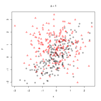
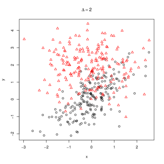
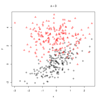
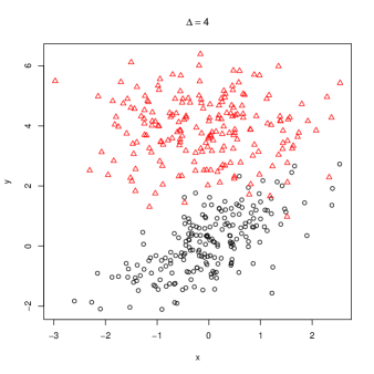
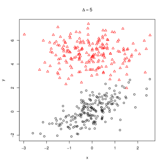
Figure 2: Typical data sets simulated from (20), illustrating varying degree of separation, where $\Delta$ indicates the Euclidean difference along the $y$-axis between group one (plotted using black circles) and group two (plotted using red triangles).

The left-hand side panel of Figure 3 plots $\overline{\text{ARI}}(\omega_{a},D_{\Delta\cdot p})$ for all of the fitted FSC models when $\Delta=1$. The right-hand side panel isolates the main species of interest for ease of viewing. For scaling purposes, these results may omit model-based clustering (i.e., $\text{FSC}_{\text{clust}}$), which often performed quite poorly. Included in these plots are the resulting average ARI values for $\text{FSC}_{\text{ARI}}$; the corresponding $\hat{\omega}_{\text{ARI}_{p}}$ values are labelled directly on the graph. The corresponding plots for $\Delta\in\{2,3,4,5\}$ are given in Figures 4 and 5.

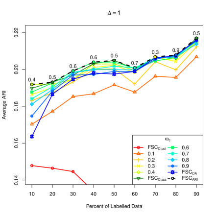
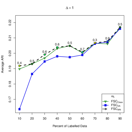
Figure 3: Average ARI values (taken over 100 runs) for FSC${}_{\omega_{a}}$ when applied to Simulation 1 with $\Delta=1$ for $\omega_{a}\in\{\bm{\omega}_{A},\hat{\omega}_{\text{ARI}_{p}}\}$ (left) and $\omega_{a}\in\{0.5,1,\hat{\omega}_{\text{ARI}_{p}}\}$ (right).

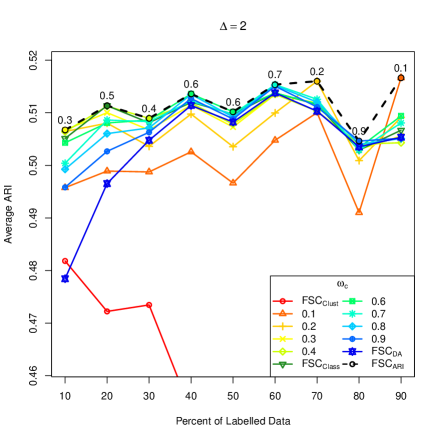
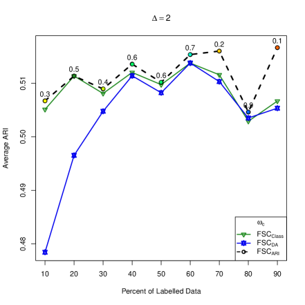
Figure 4: Average ARI values (taken over 100 runs) for FSC${}_{\omega_{a}}$ when applied to Simulation 1 with $\Delta=2$ for $\omega_{a}\in\{\bm{\omega}_{A},\hat{\omega}_{\text{ARI}_{p}}\}$ (left) and $\omega_{a}\in\{0.5,1,\hat{\omega}_{\text{ARI}_{p}}\}$ (right).

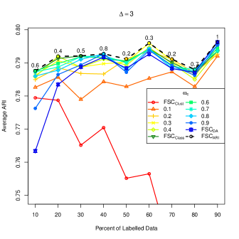
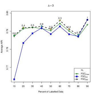
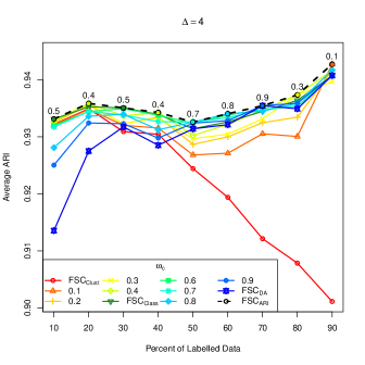
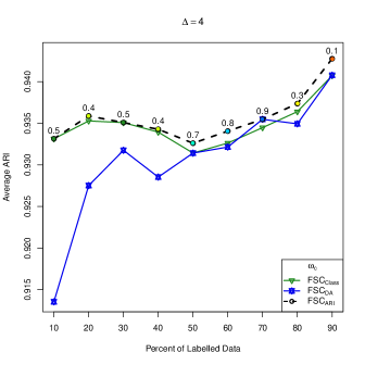
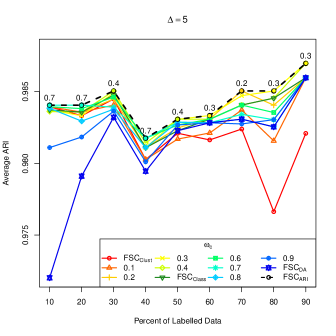
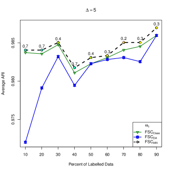
Figure 5: Average ARI values (taken over 100 runs) for FSC${}_{\omega_{a}}$ when applied to Simulation 1 with $\Delta=3,4$ and $5$, respectively, for $\omega_{a}\in\{\bm{\omega}_{A},\hat{\omega}_{\text{ARI}_{p}}\}$ (left) and $\omega_{a}\in\{0.5,1,\hat{\omega}_{\text{ARI}_{p}}\}$ (right).

When applied to the simulation with the highest degree of overlap ($\Delta=1$), $\hat{\omega}_{\text{ARI}_{p}}$ corresponds to model-based classification in three of the nine splits considered. In other words, when 20, 50 and 90% of the data are labelled, $\text{FSC}_{\text{class}}$ performs best on average. In all other cases, there exists a ‘non-species’ value — i.e., a ${\omega_{c}}\notin\{0,0.5,1\}$ — that achieves the highest average ARI. For the remaining 36 $\hat{\omega}_{\text{ARI}_{p}}$ values (nine values of $p$ times four values of $\Delta$), 31 are non-species. For the remaining five cases, four correspond to model-based classification ($\text{FSC}_{\text{class}}$) and one to DA ($\text{FSC}_{\text{DA}}$). It is worth mentioning that the value of $\hat{\omega}_{\text{ARI}_{p}}$ is less than 0.5 in 18 of the 31 cases. These cases illustrate how softening the role of labelled observations can actually lead to an increase in classification performance. For instance, the largest gain in ARI is observed at $\Delta=2$ and $p=90$, where $\text{FSC}_{0.1}$ produces an average ARI of 0.517. In comparison, $\text{FSC}_{\text{clust}}$, $\text{FSC}_{\text{class}}$, and $\text{FSC}_{\text{DA}}$ yield average ARI values of 0.364, 0.507, and 0.505, respectively. Although the majority of these runs show that non-species tend to produce the highest average ARI scores, we remark that not much difference is observed between $\text{FSC}_{\text{class}}$ and $\text{FSC}_{\text{ARI}}$. This simulation seems to suggest that when the postulated model is correct, intermediate weights do not offer a significant improvement over $\text{FSC}_{\text{class}}$. The next simulation investigates the case in which the model is misspecified.

5.2 Simulation 2

In this section, we consider 100 simulations generated from a three-component bivariate ‘restricted’ skew-$t$ mixture (cf. Vrbik and McNicholas, 2012; Lee and McLachlan, 2013). The component densities are specified to have locations $\bm{\xi}_{1}=(0\quad 0)^{\top},\bm{\xi}_{2}=(6\quad 18)^{\top},\bm{\xi}_{3}=(4\quad 2)^{\top}$; skewness $\bm{\lambda}_{1}=(2\quad 4)^{\top}$, $\bm{\lambda}_{2}=(-2\quad 4)^{\top}$, $\bm{\lambda}_{3}=(2\quad 4)^{\top}$; degrees of freedom $\nu_{1}=10,\nu_{2}=8,\nu_{3}=70$; and scale matrices

$$\bm{\Sigma}_{1}=\left(\begin{array}[]{ccc}0.4&0.2\\ 0.2&0.5\end{array}\right),\qquad\bm{\Sigma}_{2}=\left(\begin{array}[]{ccc}1&0.5\\ 0.5&1\end{array}\right),\qquad\bm{\Sigma}_{3}=\left(\begin{array}[]{ccc}0.2&0\\ 0&0.3\end{array}\right).$$

Each data set $D_{rp}$ $(r=1,\dots,100,p=10,20,\dots,90)$ contains 600 observations ($n_{1}=200$, $n_{2}=300$, $n_{3}=100$). Typical simulated data sets with 20% ($p=20$) and 60% ($p=60$) labelled observations, respectively, are given in Figure 6.

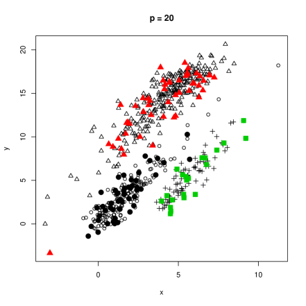
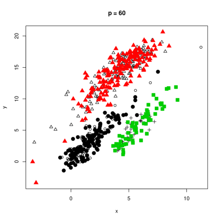
Figure 6: Scatter plots for a typical data set simulated according to Simulation 2 with 20% labelled observations (left) and 60% labelled observations (right). Labelled observations are denoted by bold symbols and color represents component membership.

In this simulation, the average ARI values (Figure 7) show that FSC performs better for larger values of ${\omega_{c}}$ when $p<70$. After this threshold, there is little difference in performance between the competing methods. As seen in Figure 7, when 10% of the observations are labelled, $\text{FSC}_{\text{class}}$ — which obtains an average ARI score of 0.868 — performs worse than $\text{FSC}_{\text{DA}}$ $(\overline{\text{ARI}}(1,D_{\cdot 10})=0.924)$ and $\text{FSC}_{\text{ARI}}$ ($\overline{\text{ARI}}(\hat{\omega}_{\text{ARI}_{p}}{},D_{\cdot 10})=0.941)$. $\text{FSC}_{\text{DA}}$ and $\text{FSC}_{\text{class}}$ are the optimal models when 50 and 70% of the data, respectively, are labelled. As indicated by the plotted values of $\hat{\omega}_{\text{ARI}_{p}}$, some cases ($p=10,20,30,40,50,80$) benefit from emphasizing the relative role of $D_{\text{L}}$ over $D_{\text{u}}$, whereas other cases ($p=90$) perform better when the opposite is true. The remaining split (when $p=70$) results in an optimum value of $\hat{\omega}_{\text{ARI}_{p}}=0.5$, indicating that $D_{\text{L}}$ and $D_{\text{u}}$ are weighted equally when building the classifier.

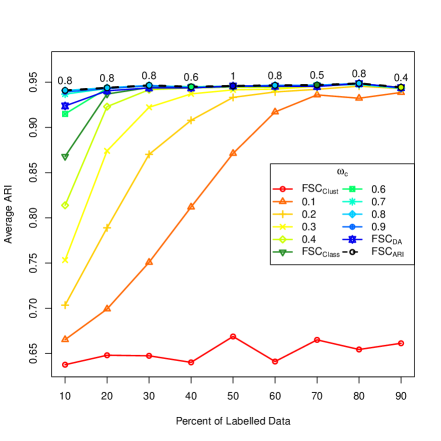
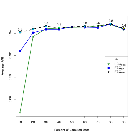
Figure 7: Average ARI values (taken over 100 runs) for FSC${}_{\omega_{a}}$ when applied to Simulation 2 for $\omega_{a}\in\{\bm{\omega}_{A},\hat{\omega}_{\text{ARI}_{p}}\}$ (left) and $\omega_{a}\in\{0.5,1,\hat{\omega}_{\text{ARI}_{p}}\}$ (right).

The sporadic patterns observed in these simulations demonstrate the difficulty behind obtaining a general rule for the specification of weights. We continue this investigation in Section 6 using real data.

6 Applications

In this section, we demonstrate how $\text{FSC}_{\omega_{a}}$ with $\omega_{a}\in\bm{\omega}_{A}$ compares with the three species of classification when applied to three real data sets. For each data set, 100 random splits are considered; again, we use $p=10,20,\dots,90.$ As in Section 5.1, the information for each run $r$ with $p\%$ labelled is stored in $D_{rp}$ for $r=1,2,\dots,100,p=10,20,\dots,90$. The resulting average ARI values for the competing methods are calculated using (19).

6.1 Italian Wine Data

The Italian wine data (Forina et al., 1986) consist of 13 chemical and physical properties of 178 wines from three different grape cultivars. This data set can be accessed through the gclus package (Hurley, 2012) for R (R Core Team, 2015). The values of $\overline{\text{ARI}}(\omega_{a},D_{\cdot p})$ for the competing methods are plotted in Figure 8. Note that data are too scarce to run $\text{FSC}_{\text{DA}}$ on less than 30% of the data. Consequently, the support of $\text{FSC}_{\text{DA}}$ is the set $\{30,40,\dots,90\}$. Similarly, $\text{FSC}_{\text{clust}}$ is only supported for $p\in\{10,20,\dots,70\}$.

When $p\leq 50$, $\text{FSC}_{\text{class}}$ performs better than $\text{FSC}_{\text{DA}}$; however, when more than half of the data are labelled, $\text{FSC}_{\text{DA}}$ outperforms $\text{FSC}_{\text{class}}$ (Figure 8). The clustering results obtained by $\text{FSC}_{\text{ARI}}$ are consistently better than for any species of classification, hence all values of $\hat{\omega}_{\text{ARI}_{p}}$ — as indicated by the labels in Figure 8 — are non-species. In fact, for all but one split ($p=90)$, the optimal weight is 0.8. The largest gain in performance can be seen at $p=40$, where $\text{FSC}_{{0.8}}$ attains an average ARI of 0.926. In comparison, the average ARI values attained by $\text{FSC}_{\text{clust}}$, $\text{FSC}_{\text{class}}$, and $\text{FSC}_{\text{DA}}$ are 0.457, 0.857, and 0.760, respectively.

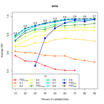
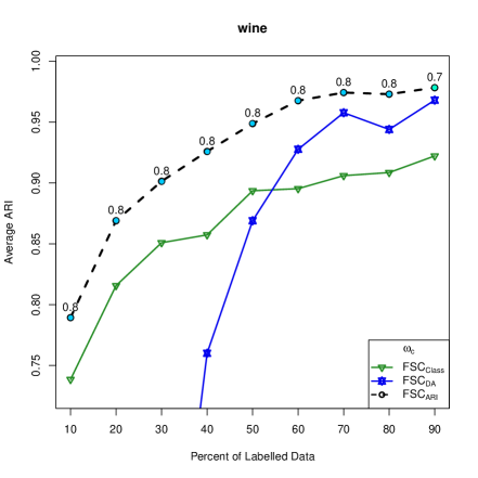
Figure 8: Average ARI values (taken over 100 runs) for FSC${}_{\omega_{a}}$ when applied to the wine data for $\omega_{a}\in\{\bm{\omega}_{A},\hat{\omega}_{\text{ARI}_{p}}\}$ (left) and $\omega_{a}\in\{0.5,1,\hat{\omega}_{\text{ARI}_{p}}\}$ (right).

6.2 Crabs Data

The crabs data (Campbell and Mahon, 1974) contain measurements on the frontal lobe size, rear width, carapace length, carapace width, and body depth of four different types of crab. This data set can be accessed through the MASS package (Venables and Ripley, 2002) for R. As seen in Figure 9, model-based classification consistently outperforms DA. Furthermore, $\text{FSC}_{\text{class}}$ gives comparable performance to $\text{FSC}_{\text{ARI}}$ for $p\geq 20$. When $p=10$, slight gains in ARI can be seen by adopting FSC with $\omega_{a}=0.6$. Namely, $\text{FSC}_{0.6}$, $\text{FSC}_{\text{class}}$, and $\text{FSC}_{\text{clust}}$ obtain $\overline{\text{ARI}}(\omega_{a},D_{\cdot p})$ values of 0.805, 0.766, and 0.172, respectively. Note that there are insufficient data to run $\text{FSC}_{\text{DA}}$ with only 10% labelled observations. Unlike the previous example, two of the optimal choices for ${\omega_{c}}$ correspond to a particular species of classification; namely, when $p=50,60$, $\text{FSC}_{\text{ARI}}$ is equivalent to $\text{FSC}_{\text{class}}$. For all other values of $p$, $\hat{\omega}_{\text{ARI}_{p}}$ is either 0.6 (when $p=10,20,30,40$) or 0.4 (when $p=70,80,90$), indicating more and less weight, respectively, on labelled observations.

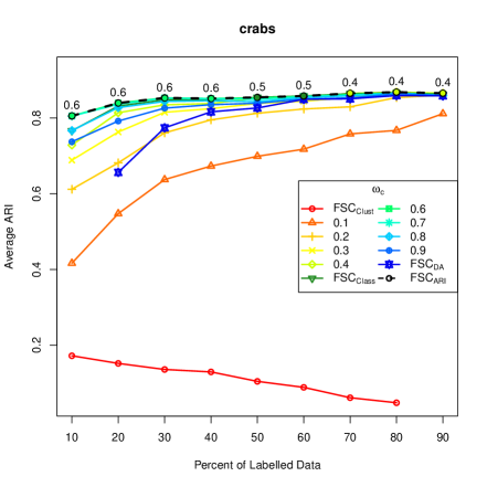
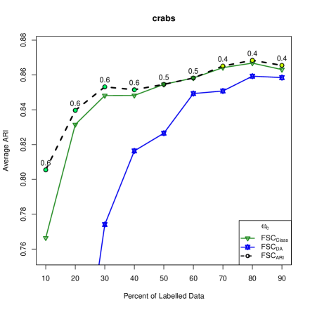
Figure 9: Average ARI values (taken over 100 runs) for FSC${}_{\omega_{a}}$ when applied to the crabs data for $\omega_{a}\in\{\bm{\omega}_{A},\hat{\omega}_{\text{ARI}_{p}}\}$ (left) and $\omega_{a}\in\{0.5,1,\hat{\omega}_{\text{ARI}_{p}}\}$ (right).

6.3 Iris Data

The iris data set contains the length and width, in centimetres, of the sepal and petals of three species of irises (Anderson, 1935; Fisher, 1936). The iris data are among the base data sets available in R. The average ARI produced by $\text{FSC}_{\text{ARI}}$ consistently outperforms all three species (Figure 10). For example, $\text{FSC}_{0.2}$ yields an average ARI of 0.929 when $p=90$ whereas $\text{FSC}_{\text{clust}}$, $\text{FSC}_{\text{class}}$, and $\text{FSC}_{\text{DA}}$ yield average ARIs of 0.749, 0.903, and 0.903, respectively. Note that when $p\leq 30$, all values of $\hat{\omega}_{\text{ARI}_{p}}$ are above 0.5, meaning more weight is given to $D_{\text{L}}$. On the contrary, when more than 30% of observations are labelled, the optimal weights are small ($\hat{\omega}_{\text{ARI}_{p}}$ = 0.1 or 0.2). This indicates that enhancing the role of $D_{\text{u}}$ over $D_{\text{L}}$ in FSC can lead to an increase in classification performance.

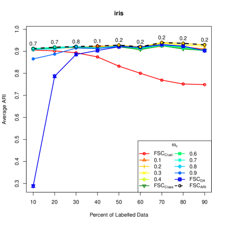
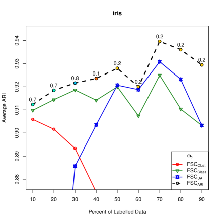
Figure 10: Average ARI values (taken over 100 runs) for FSC${}_{\omega_{a}}$ when applied to the iris data for $\omega_{a}\in\{\bm{\omega}_{A},\hat{\omega}_{\text{ARI}_{p}}\}$ (left) and $\omega_{a}\in\{0,0.5,1,\hat{\omega}_{\text{ARI}_{p}}\}$ (right).

7 Conclusion

Herein, a flexible classification paradigm, FSC, has been introduced. Constructed by adding weights to the traditional likelihood for semi-supervised classification, FSC allows any level of supervision ranging from unsupervised to supervised, with three levels coinciding with widely known species (unsupervised, semi-supervised, and supervised). We illustrated the FSC approach on real and simulated data, and explored situations where FSC can advantageously be employed. Model-based classification (i.e., $\text{FSC}_{\text{class}}$) proved competitive in some cases; however, for the majority of settings there existed a value of ${\omega_{c}}\notin\{0,0.5,1\}$ for which $\text{FSC}_{\omega_{c}}$ outperformed the three species, namely, supervised ($\text{FSC}_{\text{DA}}$), semi-supervised ($\text{FSC}_{\text{class}}$), and unsupervised classification ($\text{FSC}_{\text{clust}}$).

Of course, the efficacy of FSC depends on the challenging task of specifying the weight ${\omega_{c}}$. The optimal value for ${\omega_{c}}$ — as determined by the average ARI from a candidate set of potential weights $\bm{\omega}_{A}$ — has proven to be fairly unpredictable, reflecting the complicated role that unlabelled and labelled data can have on building a classifier. Specifically, we observed four scenarios: (a) $0<\hat{\omega}_{\text{ARI}_{p}}<0.5$; (b) $\hat{\omega}_{\text{ARI}_{p}}=0.5$; (c) $0.5<\hat{\omega}_{\text{ARI}_{p}}<1$; and (d) $\hat{\omega}_{\text{ARI}_{p}}=1$. Scenarios (a) and (c) correspond to cases where the best model is obtained by emphasizing the relative roles of unlabelled and labelled data, respectively. Scenario (b) corresponds to the optimal model occurring at $\text{FSC}_{\text{class}}$. Scenario (d) coincides with $\text{FSC}_{\text{DA}}$, and occurs when the inclusion of unlabelled data leads to a decrease in classification performance. We never observed a scenario in which $\hat{\omega}_{\text{ARI}_{p}}=0$ was optimal.

In conclusion, FSC provides a flexible framework that unites the three species of classification (i.e., supervised, semi-supervised, and unsupervised) and promotes the exploration and development of weighted likelihood techniques. Moving forward, the major challenge is to devise an automated way of selecting ${\omega_{c}}$ that, ideally, never performs worse than the three species. To this end, the development of a data-driven selection criterion is a subject of ongoing investigation.

Apart from the delicate issue of weight specification, numerous expansions can be explored within the FSC framework. For example, one could extend FSC to include the special case where known class labels ($\mathds{Z}_{1}$), rather than labeled observation pairs ($D_{\text{L}}=\{\mathds{X}_{1},\mathds{Z}_{1}\}$), are ignored. This might be accomplished by having separate weights for $\mathds{X}_{i}$ and $\mathds{Z}_{i}$. Another avenue of research involves adapting these models so that they may be applied to situations where observations are systematically unlabelled. In this way, FSC could help offset the potential bias introduced by systematic missingness. Expanding on this idea, one might include the possibility of more than two sources of data. For instance, in addition to unlabelled and labelled data we may allow for a third source, perhaps comprised of outliers or data suspected to be mislabelled. We believe the methods presented in this paper are simply the forerunners to a different approach to classification, one based upon the weighted likelihood.

Acknowledgements

This work was supported by an Ontario Graduate Scholarship (Vrbik), an Early Researcher Award from the Government of Ontario (McNicholas), and a Discovery Grant from the Natural Sciences and Engineering Research Council of Canada (McNicholas).

References

- Akaike (1973) Akaike, H. (1973). Information theory and an extension of the maximum. In Second International Symposium on Information Theory, pp. 267–281.
- Anderson (1935) Anderson, E. (1935). The irises of the Gaspé Peninsula. Bulletin of the American Iris Society 59, 2–5.
- Andrews et al. (2011) Andrews, J. L., P. D. McNicholas, and S. Subedi (2011). Model-based classification via mixtures of multivariate t-distributions. Computational Statistics and Data Analysis 55(1), 520–529.
- Baluja (1998) Baluja, S. (1998). Probabilistic modeling for face orientation discrimination: Learning from labeled and unlabeled data. In Neural Information Processing Systems (NIPS ‘98), pp. 854–860.
- Baranchik (1970) Baranchik, A. J. (1970). A family of minimax estimators of the mean of a multivariate normal distribution. The Annals of Mathematical Statistics 41, 642–645.
- Baudry et al. (2010) Baudry, J.-P., A. E. Raftery, G. Celeux, K. Lo, and R. Gottardo (2010). Combining mixture components for clustering. Journal of Computational and Graphical Statistics 19(2), 332–353.
- Berry (1994) Berry, J. C. (1994). Improving the James-Stein estimator using the Stein variance estimator. Statistics and Probability Letters 20(3), 241–245.
- Biernacki et al. (2000) Biernacki, C., G. Celeux, and G. Govaert (2000). Assessing a mixture model for clustering with the integrated completed likelihood. IEEE Transactions on Pattern Analysis and Machine Intelligence 22(7), 719–725.
- Campbell and Mahon (1974) Campbell, N. A. and R. J. Mahon (1974). A multivariate study of variation in two species of rock crab of genus Leptograpsus. Australian Journal of Zoology 22, 417–425.
- Castelli and Cover (1996) Castelli, V. and T. M. Cover (1996). The relative value of labeled and unlabeled samples in pattern recognition with an unknown mixing parameter. IEEE Transactions on Information Theory 42(6), 2102–2117.
- Cozman et al. (2003) Cozman, F. G., I. Cohen, and M. C. Cirelo (2003). Semi-supervised learning of mixture models. In International Conference on Machine Learning (ICML 2003), pp. 99–106.
- Dempster et al. (1977) Dempster, A. P., N. M. Laird, and D. B. Rubin (1977). Maximum likelihood from incomplete data via the EM algorithm. Journal of the Royal Statistical Society: Series B 39(1), 1–38.
- Edwards and Cavalli-Sforza (1965) Edwards, A. W. F. and L. L. Cavalli-Sforza (1965). A method for cluster analysis. Biometrics 21, 362–375.
- Fisher (1936) Fisher, R. A. (1936). The use of multiple measurements in taxonomic problems. Annals of Eugenics 7(Part II), 179–188.
- Forina et al. (1986) Forina, M., C. Armanino, M. Castino, and M. Ubigli (1986). Multivariate data analysis as a discriminating method of the origin of wines. Vitis 25, 189–201.
- Hartigan and Wong (1979) Hartigan, J. A. and M. A. Wong (1979). Algorithm AS 136: A k-means clustering algorithm. Journal of the Royal Statistical Society: Series C 28(1), 100–108.
- Hennig (2010) Hennig, C. (2010). Methods for merging Gaussian mixture components. Advances in Data Analysis and Classification 4, 3–34.
- Hu (1994) Hu, F. (1994). Relevance Weighted Smoothing and a New Bootstrap Method. Ph. D. thesis, University of British Columbia.
- Hu (1997) Hu, F. (1997). The asymptotic properties of the maximum-relevance weighted likelihood estimators. The Canadian Journal of Statistics 25, 45–59.
- Hu and Zidek (2001) Hu, F. and J. V. Zidek (2001). The relevance weighted likelihood with applications. In Empirical Bayes and Likelihood Inference, pp. 211–235. Springer.
- Hu and Zidek (2002) Hu, F. and J. V. Zidek (2002). The weighted likelihood. The Canadian Journal of Statistics 30(3), 347–371.
- Hubert and Arabie (1985) Hubert, L. and P. Arabie (1985). Comparing partitions. Journal of Classification 2, 193–218.
- Hurley (2012) Hurley, C. (2012). gclus: Clustering Graphics. R package version 1.3.1.
- James and Stein (1961) James, W. and C. Stein (1961). Estimation with quadratic loss. In Proceedings of the Fourth Berkeley Symposium on Mathematical Statistics and Probability, Volume 1, pp. 361–379.
- Kawakita and Takeuchi (2014) Kawakita, M. and J. Takeuchi (2014). Safe semi-supervised learning based on weighted likelihood. Neural Networks 53, 146–164.
- Kullback and Leibler (1951) Kullback, S. and R. A. Leibler (1951). On information and sufficiency. The Annals of Mathematical Statistics 22(1), 79–86.
- Lee and McLachlan (2013) Lee, S. and G. McLachlan (2013). On mixtures of skew normal and skew t-distributions. Advances in Data Analysis and Classification 7(3), 241–266.
- McCallum and Nigam (1998) McCallum, A. and K. Nigam (1998). Employing EM and pool-based active learning for text classification. In Proceedings of the 15th International Conference on Machine Learning (ICML 1998), Madison, pp. 350–358.
- McNicholas (2010) McNicholas, P. D. (2010). Model-based classification using latent Gaussian mixture models. Journal of Statistical Planning and Inference 140(5), 1175–1181.
- Nigam et al. (2000) Nigam, K., A. K. McCallum, S. Thrun, and T. Mitchell (2000). Text classification from labeled and unlabeled documents using EM. Machine Learning 39(2–3), 103–134.
- Planté (2008) Planté, J. F. (2008). Adaptive Likelihood Weights and Mixtures of Empirical Distributions. Ph. D. thesis, The University of British Columbia.
- Planté (2009) Planté, J. F. (2009). Asymptotic properties of the MAMSE adaptive likelihood weights. Journal of Statistical Planning and Inference 139(7), 2147–2161.
- R Core Team (2015) R Core Team (2015). R: A Language and Environment for Statistical Computing. Vienna, Austria: R Foundation for Statistical Computing.
- Ratsaby and Venkatesh (1995) Ratsaby, J. and S. S. Venkatesh (1995). Learning from a mixture of labeled and unlabeled examples with parametric side information. In Proceedings of the Eighth Annual Conference on Computational Learning Theory, pp. 412–417. ACM.
- Schwarz (1978) Schwarz, G. (1978). Estimating the dimension of a model. The Annals of Statistics 6(2), 461–464.
- Scott and Symons (1971) Scott, A. J. and M. J. Symons (1971). Clustering methods based on likelihood ratio criteria. Biometrics 27, 387–397.
- Sokolovska et al. (2008) Sokolovska, N., O. Cappé, and F. Yvon (2008). The asymptotics of semi-supervised learning in discriminative probabilistic models. In Proceedings of the 25th International Conference on Machine Learning, pp. 984–991. ACM.
- Stein (1956) Stein, C. (1956). Inadmissibility of the usual estimator for the mean of a multivariate normal distribution. In Proceedings of the Third Berkeley Symposium on Mathematical Statistics and Probability, Volume 1, pp. 197–206.
- Steinley (2004) Steinley, D. (2004). Properties of the Hubert-Arabie adjusted Rand index. Psychological Methods 9(3), 386.
- Strawderman (1973) Strawderman, W. E. (1973). Proper Bayes minimax estimators of the multivariate normal mean vector for the case of common unknown variances. The Annals of Statistics 6, 1189–1194.
- Vandewalle et al. (2008) Vandewalle, V., C. Biernacki, G. Celeux, and G. Govaert (2008). Are unlabeled data useful in semi-supervised model-based classification? Combining hypothesis testing and model choice. In Proceedings of the first joint meeting of the Société Francophone de Classification and the Classification and Data Analysis Group of SIS, pp. 433–436.
- Venables and Ripley (2002) Venables, W. N. and B. D. Ripley (2002). Modern Applied Statistics with S (Fourth ed.). New York: Springer.
- Vrbik and McNicholas (2012) Vrbik, I. and P. D. McNicholas (2012). Analytic calculations for the EM algorithm for multivariate skew-t mixture models. Statistics and Probability Letters 82(6), 1169–1174.
- Vrbik and McNicholas (2014) Vrbik, I. and P. D. McNicholas (2014). Parsimonious skew mixture models for model-based clustering and classification. Computational Statistics and Data Analysis 71, 196–210.
- Wald (1949) Wald, A. (1949). Note on the consistency of the maximum likelihood estimate. The Annals of Mathematical Statistics 20(4), 595–601.
- Wang (2001) Wang, S. X. (2001). Maximum Weighted Likelihood Estimation. Ph. D. thesis, University of British Columbia.
- Wang et al. (2004) Wang, S. X., C. van Eeden, and J. V. Zidek (2004). Asymptotic properties of maximum weighted likelihood estimators. Journal of Statistical Planning and Inference 119, 37–54.
- Wang and Zidek (2005) Wang, S. X. and J. V. Zidek (2005). Selecting likelihood weights by cross-validation. Annals of Statistics 33, 463–501.
- Wang (2006) Wang, X. (2006). Approximating Bayesian inference by weighted likelihood. Canadian Journal of Statistics 34(2), 279–298.
- Wolfe (1965) Wolfe, J. H. (1965). A computer program for the maximum likelihood analysis of types. Technical Bulletin 65-15, U.S. Naval Personnel Research Activity.