Colour gradients of high-redshift Early-Type Galaxies from hydrodynamical monolithic models

Abstract

We analyze the evolution of colour gradients predicted by the hydrodynamical models of early type galaxies (ETGs) in Pipino et al. (2008), which reproduce fairly well the chemical abundance pattern and the metallicity gradients of local ETGs. We convert the star formation (SF) and metal content into colours by means of stellar population synthetic model and investigate the role of different physical ingredients, as the initial gas distribution and content, and $\epsilon_{\rm SF}$, i.e. the normalization of SF rate. From the comparison with high redshift data, a full agreement with optical rest-frame observations at $z\mathrel{\hbox to0.0pt{\lower 3.5pt\hbox{\hskip 0.5pt$\sim$}\hss}\raise 0.5pt\hbox{$<$}}1$ is found, for models with low $\epsilon_{\rm SF}$, whereas some discrepancies emerge at $1<z<2$, despite our models reproduce quite well the data scatter at these redshifts. To reconcile the prediction of these high $\epsilon_{\rm SF}$ systems with the shallower colour gradients observed at lower z we suggest intervention of 1-2 dry mergers. We suggest that future studies should explore the impact of wet galaxy mergings, interactions with environment, dust content and a variation of the Initial Mass Function from the galactic centers to the peripheries.

1 Introduction

Radial variations in ages and metallicities of stellar populations (SPs) have been shown to be efficient tools to discriminate among different galaxy formation scenarios. Recently, a plethora of studies have dedicated attention to the analysis of gradients in colours and absorption features for wide samples of local early-type galaxies (ETGs; e.g. Spolaor et al. 2009; Kuntschner et al. 2010; Rawle et al. 2010; Spolaor et al. 2010; Tortora et al. 2010, herafter T+10; Tortora et al. 2011), deriving SP gradients by means of stellar population synthesis (SPS) analysis. Whilst these works consistently find a decrease in the metallicity at large radii as the cause of both line-strength and colour gradients, the scatter in the galaxy properties at fixed stellar mass still prevent from deriving robust constraints on the competing galaxy formation models on the market (Pipino et al. 2010).

For instance, a well known class of these models is represented by the so-called monolithic models. Steep metallicity gradients ($\sim-0.5\,\rm dex$ per decade variation in radius) are expected from classical dissipative collapse models (e.g. Larson 1974; Carlberg 1984) and their revised versions starting from semi-cosmological initial conditions (e.g. Kawata 2001, Kobayashi 2004). These metallicity gradients arise because the stars form everywhere in the collapsing cloud and then remain in orbit with a little inward motion whereas the gas falls down because of dissipation. This falling gas contains the new metals ejected by evolving stars so that a metallicity gradient develops in the gas. As stars continue to form, their composition reflects the gaseous abundance gradient. Pipino et al. (2008) and Pipino et al. (2010) have shown that monolithic hydrodynamical models can be able to satisfy different local correlations, as the mass–metallicity and the mass–$[\alpha/Fe]$ relations and produce metallicity gradients of $\sim-0.3\,\rm dex$, consistent with several observational samples (Spolaor et al. 2009; Spolaor et al. 2010; Kuntschner et al. 2010; Rawle et al. 2010; Tortora et al. 2010; La Barbera et al. 2011). These results have been possible thanks to the requirement, fulfilled by the models, that the stars produced have high average $[\alpha/Fe]$ in the cores and thus short SF, and smaller age gradients.

It is however important to note that some simulations in the suite by Pipino et al. (2008) and Pipino et al. (2010) still feature very steep metallicity gradients of $\sim-0.5\,\rm dex$, explaining the observed scatter in massive ETGs (e.g. Tortora et al. 2010) in terms of variations in the initial conditions and in particular in the efficiency of star formation (SF) processes. These authors explain the metallicity gradients in massive ETGs without recurring to strong AGN feedback (Tortora et al. 2009a; Tortora et al. 2010), which have been suggested to flatten the gradients. Cosmological simulations require that the formation of massive galaxies must include at least a few “dry mergers” (De Lucia et al. 2006): these would flatten any pre-existing metallicity gradients (Bekki & Shioya 1999; Kobayashi 2004; Di Matteo et al. 2009). Only if the pre-existing gradients in the progenitors of a merging system are enough steep, it is possible that the descendant model galaxy will match the observed values at $z\sim$0 (Carollo et al. 1993; Davies et al. 1993; Sánchez-Blázquez et al. 2006; Sánchez-Blázquez et al. 2007; Annibali et al. 2007; Ogando et al. 2005; Spolaor et al. 2009; Tortora et al. 2010). Clearly, observations of local massive ellipticals do not have enough constraining power as models improve in complexity, each of them featuring a mixture of different channels for galaxy formation, In order to break such degeneracies, both observational and numerical studies at different environments and redshift are needed.

From the observational point of view, to have a full picture is necessary to analyze colour and SP gradients in higher-redshift galaxies. Unfortunately, the available datasets cover local environments and only few studies allow the investigation of colour and SP gradients at higher redshifts (La Barbera et al. 2004; Tamura et al. 2000; Tamura & Ohta 2000; Menanteau et al. 2001; Ferreras et al. 2009; Guo et al. 2011; Gargiulo et al. 2011, 2012; Welikala & Kneib 2012).

In the present paper we further exploit a sample of the hydrodynamical models for massive ETGs in Pipino et al. (2008), we transform the SPs of the model predictions (evolution in metal content and SF history) into magnitudes and colours using the SPS in Bruzual & Charlot (2003). This approach allows us to compare our models with observed colour gradients and avoid typical systematics (as the age-metallicity degeneracy) plaguing the SPS fitting. We will concentrate on two different aspects:

1. the evolution with redshift of the colour gradients and the analysis of the role of the initial conditions of the models, as the initial gas density distribution, its mass content, and the rate of SF processes;

2. the comparison with observed color gradients at low/moderate redshift ($z<1$) and high redshift (i.e. $z>1$),

with the aim of testing the consequences of assuming one particular model, and to make predictions to be validated with future data.

The paper is organized as follows. In Sect. 2 we discuss the simulation setup and the main characteristics of the models. The evolution with redshift of the colour gradients in the rest-frame of the galaxies is shown in Sect. 3, while the comparison with high redshift observations and systematics are analyzed in Sect. 4. In Sect. 5 we discuss our results within a wider formational scheme and conclusions are outlined in Sect. 6.

Table 1: Model input and output parameters, from Pipino et al. (2008). Ei codes identify model galaxies. Models E1, E2, E3 and E4 correspond to Ma1, Mb3, Mb4 and LB in Pipino et al. (2008), respectively. Columns report, as imput parameters: 1) the name of the model, 2) the initial central gas density $\rho_{\rm 0,gas}$, 3) the initial gas profile, 4) the SF parameter $\epsilon_{\rm SF}$ (see Eq. (1)) and 5) the DM mass $M_{\rm DM}$, and the final ($z=0$) output parameters: 6) the stellar mass $M_{\star}$, 7) the half-mass radius $r_{\rm 1/2}$, 8) [O/Fe] of SPs in the galactic core, 9) age gradient, $\nabla_{\rm age}$, 10) Z gradient, $\nabla_{\rm Z}$. Gradients in columns 9) and 10) are calculated accordingly to Pipino et al. (2008) and Pipino et al. (2010) as $\nabla_{X}=(\log X_{\rm core}-\log X_{\rm e})/(\log r_{\rm core}-\log\mbox{$r_{\rm 1/2}$})$, where $\rm X=\rm Z$, $\rm age$, and $r_{\rm core}$ is set as in Table 2 in Pipino et al. (2008). The stellar and DM mass are limited to their tidal radii (see Pipino et al. (2008) for details). $\flat$ Note that, for E4, after fixing a bug, the local gradient getting out is steeper than the one shown in Pipino et al. (2008, 2010).

	Input					Output
Model	$\rho_{\rm 0,gas}$	Initial profile	$\epsilon_{\rm SF}$	$M_{\rm DM}$		$M_{\star}$	$r_{\rm 1/2}$	$[O/Fe]_{\rm core}$	$\nabla_{\rm age}$	$\nabla_{\rm Z}$
	($10^{-25}\,\rm g\,cm^{-3}$)			($10^{11}\,\rm\mbox{$M_{\odot}$}$)		($10^{10}\mbox{$M_{\odot}$}$)	(kpc)	(dex)	(dex)	(dex)
E1	0.6	IS	1	22		6.0	12	0.29	$2.8\times 10^{-4}$	-0.2
E2	0.06	flat	10	22		21	8.8	0.17	$2.3\times 10^{-3}$	-0.35
E3	0.6	flat	1	22		26	5.4	0.42	$3.6\times 10^{-4}$	-0.21
E4	0.6	flat	10	57		29	21	0.12	$6.0\times 10^{-3}$	-0.45♭

2 Simulation setup and spectral synthesis

We adopted the hydrodynamical model in Pipino et al. (2008) and Pipino et al. (2010) to predict the evolution of SF and metallicity and SPS models from Bruzual & Charlot (2003) to link the predicted SP evolution to observable quantities as colours. Below we briefly summarize the simulation specifics and typical behaviours.

2.1 Hydrodynamical model

2.1.1 General setup

We use a one-dimensional hydrodynamical model that follows the time evolution of the density of mass, momentum and internal energy of a galaxy, under the assumption of spherical symmetry. The standard gas-dynamical equations (Bedogni & D’Ercole 1986, Pipino et al. 2008) include source terms to describe the injection of total mass and energy in the gas due to the mass return and energy input from the stars, including SNIa and SNII in a self-consistent way. This allows the code to follow the hydrodynamical evolution of H, He, O and Fe in detail.

The grid in divided in 550 zones with a size ratio between adjacent zones equal to 1.03. The innermost zone is 10 pc wide. At the grid center we impose reflecting boundary condition, whereas we set outflow condition in the outermost point.

At every point of the mesh we allow the SF to occur at the following rate:

$$\Psi=\nu\rho={\epsilon_{SF}\over max(t_{cool},t_{ff})}\rho\,$$ (1)

where $t_{cool}$ and $t_{ff}$ are the local cooling and free-fall timescales, respectively, $\rho$ is the mass density and $\epsilon_{SF}$ is a suitable SF parameter that contains all the uncertainties on the timescales of the SF process. We assume that the stars do not move from the gridpoints at which they have been formed, since we expect that the stars will spend most of their time close to their apocentre.

As previously discussed in Pipino et al. (2008), very strong SN feedback can stop SF processes too early, predicting high $\alpha$-enhancement in the galactic core and a too diffuse galaxy. On the other hand, the energy input in the ISM by SN is about $5-10\%$ (Thornton et al. 1998), thus both the SNIa and SNII efficiency are assumed to be $\epsilon_{SN}=0.1$. Small variations (e.g. $\epsilon_{SN}=0.2$) do not affect the results. A Salpeter (1955) initial mass function (IMF), constant in time in the range $0.1-50M_{\odot}$, is assumed. Such IMF has been shown to reproduce the photochemical properties of elliptical galaxies (e.g., Pipino & Matteucci 2004; Pipino et al. 2008; Pipino et al. 2010). A top-heavier IMF would increase the production of SNe and enhance the SN feedback (Romeo et al. 2008), while a bottom-lighter IMF (as, e.g. Kroupa 2001) would not impact SN feedback. Although the investigation of the effects of the IMF on the model behaviors is beyond the aims of this paper, the later discussion about the IMF non–universality (Treu et al. 2010; Conroy & van Dokkum 2012; Cappellari et al. 2012a; Tortora et al. 2013) represents a further important ingredient of the galaxy evolution to take into account in future simulations. We will limit to discuss the possible effect of the IMF variation with galaxy mass in Sects. 5 and 6, when we will compare our models with real data.

2.1.2 Initial conditions

In Table 1 we show relevant properties of the 4 models we analyze, we have called E1, E2, E3 and E4. In particular, we show both a few important input parameters - that set the initial conditions and that we discuss below - and predicted quantities such as the stellar mass and $r_{\rm 1/2}$, as well as the metallicity and age gradients. We culled these four models from those run by Pipino et al. (2008, 2010) to efficiently scan the space of the setup parameters, i.e. the central gas density $\rho_{\rm 0,gas}$, the initial profile of gas distribution, the SF parameter $\epsilon_{\rm SF}$, and the initial DM content, $M_{\rm DM}$, that bracket a range of possible initial configurations in terms of amount of gas initially available, timescale of accretion/cooling of such gas and timescale of gas consumption due to star formation. Here, we briefly discuss these input parameters in detail.

• $\rho_{0,gas}$. The values for $\rho_{0,gas}$ are set in order not to limit the amount of gas in the grid, i.e. smaller than the typical baryon fraction in high density environment (McCarthy et al. 2007). E2 has a $\rho_{0,gas}$ of $10$ times smaller than the one in the other models.

• Initial profile. The gas can be initially distributed as an isothermal sphere (flagged as IS, mimicking a fast accretion of gas before the bulk of the SF begins) or a uniform distribution within the whole box (models flagged as flat). In the case E1 an IS profile is adopted, while for the other models we use the flat profile .

• $\epsilon_{\rm SF}$. The SF parameter, $\epsilon_{\rm SF}$ (Eq. (1); Pipino et al. 2008) is taken constant as a function of radius. We assume values of $1$ and $10$, which guarantee SF rates of 10-500 $M_{\odot}$/yr in massive galaxies, comparable with the observations of high redshift star forming objects. Models E1 and E3 have $\mbox{$\epsilon_{\rm SF}$}=1$, while for E2 and E4 is $\mbox{$\epsilon_{\rm SF}$}=10$.

• $M_{\rm DM}$. The adopted DM masses are $M_{\rm DM}=2.2\times 10^{12}\,\mbox{$M_{\odot}$}$ and $M_{\rm DM}=5.7\times 10^{12}\,\mbox{$M_{\odot}$}$. The DM potential has been evaluated by assuming a distribution inversely proportional to the square of the radius at large distances (Silich & Tenorio-Tagle 1998). And all these quantities have been chosen to ensure a final ratio between the mass of baryons in stars and the mass of the DM halo of around 0.1. The model E4 have the largest initial DM mass. A limitation of the model is that we assume a fixed DM potential. On the other hand, the details of the potential are not relevant for the baryonic processes as long as the DM has a characteristic radius much larger than that of the baryons (e.g. Martinelli et al. 1998). Moreover, it is still a problem for simulations to reproduce SF histories that fit the chemical abundance data, if the baryon accretion follows the DM growth (Colavitti et al. 2009; Pipino et al. 2009). A more sophisticated description of the DM will be included in future works.

We do not discuss variation in the actual starting value of the temperature, since it is less important than, e.g., the chosen $\epsilon_{SF}$ (Pipino et al. 2010). Pairs of models differ for a single parameter, such as by confronting models one-to-one will allow us to investigate the effect of the individual parameters on the simulation set-up. In particular, E1 and E3 have the same initial conditions but a different gas profile, i.e. IS and flat, respectively. E2 and E4 have the same initial gas distribution and $\epsilon_{\rm SF}$, but a different gas density in the core. E3 and E4 have the same $\rho_{\rm 0,gas}$ and gas distribution, but E4 has a larger $\epsilon_{\rm SF}$.

As extensively discussed in Pipino et al. (2010), different - but reasonable - combinations of the input parameters lead to model properties that reproduce both the overall chemical properties observed in local elliptical galaxies. Using [$<O$/Fe$>$] as tracer of [$<\alpha$/Fe$>$] (see Table 1), Pipino et al. (2010) have shown that the models adopted hereafter are satisfactorily consistent with the observations at fixed galaxy mass (Thomas et al. 2007). Indeed, these models also reproduce the lack of radial gradient in [$<\alpha$/Fe$>$]. At the same time, these simulations reproduce the mass-metallicity relation (Thomas et al. 2007) and the relation between local escape velocity and local metallicity (Scott et al. 2009). Using colour gradients we will further constrain the space of physical parameters involved.

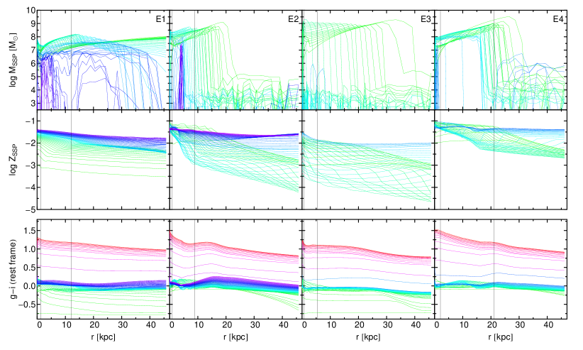
Figure 1: Stellar mass (top panels) and relative metallicity (middle panels) in SSP formed at each time step and $g-i$ colour (bottom panels), as a function of the distance from the center of galaxy. From the left to right E1, E2, E3 and E4 are shown. The vertical lines set the final $0.1\mbox{$r_{\rm 1/2}$}$ and $r_{\rm 1/2}$. The colour bar on the top sets the colour code of the curves in terms of the redshift.

2.1.3 A brief sketch of the model behaviour

Before discussing the details of the models it is worth briefly reminding their general behaviour, whereas we refer the reader to Pipino et al. (2008) for a comprehensive analysis. At times earlier than few hundred Myrs the gas is accumulating in the central regions where the density increases. The temperature drops due to cooling and, thus, the SF can proceed at very high rates. After a few hundred Myrs the gas, being heated by SN explosions, is outflowing at the largest radii, while still being accreted in the central regions. Afterwards (at times $t_{\rm gw}>0.2-1.2$ Gyr, depending on the model) a galactic wind driven by SNIa+II involves the entire galaxy. Such a behaviour is simply explained by the fact that the energy required to extract the gas from the galaxy outskirts is less than the work needed to have an outflow originating in the galactic center, leading to the correlation between metallicity and escape velocity gradient, as shown in Pipino et al. (2010). This strong wind can be maintained for several Gyrs , contributing to the ejection of the chemical elements into the surrounding medium (Pipino et al. 2002).

These models exhibit metallicity gradients in the range $-0.2,-0.4$ dex per decade in radius and negligible age gradients (cfr. Table 1). Changes in the initial conditions within the same broad formation scenario create the scatter in the predicted gradients at a single mass.

The shallower gradients predicted by this new monolithic models with respect to earlier dissipational collapse models (e.g. Larson 1974; Carlberg 1984) derives from a constraint that was not available when the original collapse models were put forward, namely that it is necessary to produce stars with high [$<\alpha$/Fe$>$] ratios inhabiting the galactic core. This turns into a need for short duration of the SF (accordingly to observations; Matteucci 1994; Thomas et al. 2005). Hence, the metal enrichment process cannot last more than 1 Gyr, leading to small age gradients even in the most massive galaxies (e.g. Tortora et al. 2010).

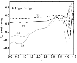
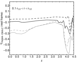
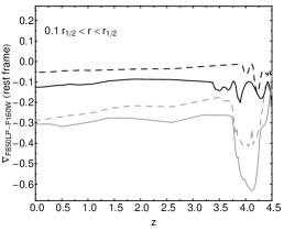
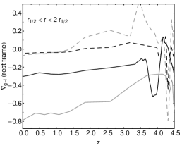
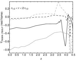
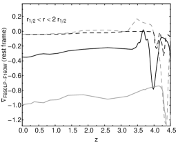
Figure 2: Gradients in the rest frame of the galaxy as a function of z for E1 (black solid line), E2 (gray dashed line), E3 (black dashed line) and E4 (gray solid line). From the left to the right $\nabla_{\rm g-i}$, $\nabla_{\rm F606W-F850LP}$ and $\nabla_{\rm F850LP-F160W}$ are plotted. In the top (bottom) panels the gradients are calculated assuming $0.1\mbox{$r_{\rm 1/2}$}<r<\mbox{$r_{\rm 1/2}$}$ ($\mbox{$r_{\rm 1/2}$}<r<2\mbox{$r_{\rm 1/2}$}$).

2.2 Stellar population analysis

To derive quantities that can be compared with observations we use a set of “single burst” stellar population synthesis (SPS) spectra from Bruzual & Charlot (2003, hereafter BC03) as the building blocks of our composite SPs. To match the assumptions in the simulations a Salpeter (1955) IMF is adopted, metallicity, $Z$, ranging within $0.0001-0.05$ and ages, t, in the interval $0.001-15\,\rm Gyr$ are used. To improve the sensitivity of the results to the small differences in both $Z$ and ages, we have adopted a “mesh refinement” procedure which interpolates the synthetic models.

For each galaxy, and at each radius, we discretize the star formation history. Specifically, we link a BC03 SED to the $i-th$ SSP formed at a time $t_{i}$, with a given $Z_{\rm SSP}$ and a mass $M_{\rm SSP}$, assuming that the burst that created it is instantaneous. We assume that at times $t>t_{i}$ it passively evolves till present day. Thus, at each time and radius, we have a collection of SPS which we weigh according to the mass $M_{\rm SSP}$ assembled in every previous timestep, and sum to derive the composite galaxy spectrum at that fixed time and spatial position. Suitably convolving the spectral response of filters with the SED, we derive the surface brightness and magnitudes. In the present paper we discuss the results for several SDSS and HST pass bands, which will be compared with observations from the literature. We apply this procedure to the SSPs formed in spherical annuli with radii from 0 to $\sim 45$ kpc, to reconstruct the colour profiles and average colours. To investigate spurious systematics arising from the assumption of a specific SPS prescription we have also adopted an updated version of BC03 models (BC03-updated, hereafter; Eminian et al. 2008) and Maraston (2005, M05 hereafter) models, which include an improved treatment of the thermally-pulsing asymptotic giant branch phase (TP-AGB).

We discuss the colour profile $(X-Y)(r)$ where $X$ and $Y$ are the two bands considered. The colour gradient is defined as the angular coefficient of the relation $X-Y$ vs $\log r$, $\displaystyle\nabla_{X-Y}=\frac{\delta(X-Y)}{\delta\log r}$, measured in $\rm mag/dex$ (omitted in the following unless needed for clarity). To take the analysis as simple as possible we avoid any projection of galaxy light distribution, calculating the gradients using the 3D distribution and the spherical half-mass radius $r_{\rm 1/2}$. We have verified that for the scope of this paper the impact of this assumption is small, leaving unaffected our conclusions. In the worst cases, the projection will flatten the steepest gradients of, at most $0.1-0.2$ mag/dex. The fit of each color profile is performed in different radial ranges; in particular, to homogeneously compare with observations we often use the range $0.1\mbox{$r_{\rm 1/2}$}\leq r\leq\mbox{$r_{\rm 1/2}$}$.

The spherical assumption is a possible limitation for our models, since calculating the colour gradients of more realistic triaxial or oblate systems along different lines of sights would produce different gradients. The inclusion of more complex geometries is a natural step forward in this kind of analyses. For the present paper, we have limited our models to be as simple as possible, demonstrating that they can satisfactorily reproduce key low-redshift observations (Pipino et al. 2008, 2010). Under the assumption that the galaxy formation is fairly homogeneous, as we expect to be in the case of an isolated galactic system, the presence of asymmetries in mass distribution is expected to be marginal. In this case it is instructive to study if any observed variation in the gradient can be traced back to variations in physical quantities, before taking the further step of relaxing the assumption of galaxies evolving homogenously and in isolation and introducing the effect of the merging on the gradient distribution. We note that, even in this last case, Hopkins et al. (2009) have demonstrated that gradients along different lines of sights of remnants of disk galaxies mergers present a scatter around the median gradient which is less that 0.1, namely smaller than the observed scatter at a fixed galaxy mass.

On the observational side, while it is true that age/metallicity profiles taken at two different position angles may differ (e.g. Fig. 7 in Carollo et al. 1993), and we are aware that inhomogeneities and structures are clear also in 2-dimensional metallicity maps of ellipticals (e.g. Kuntschner et al. 2006), these are plausibly second-order effects, related to the particular assembly history of a given galaxy and contributing very little to the scatter in the data.

3 Colour gradients and evolution with redshift

In this section, we discuss the main predictions of our simulations, concentrating on the evolution of colour profiles and colour gradients in the rest-frame of the galaxy, which provide us with information about the physics behind the simulations and the link with observables.

The profiles for the mass formed, metallicity and $g-i$ color for the four models are shown in Fig. 1, whereas the gradients $\nabla_{\rm g-i}$, $\nabla_{\rm F606W-F850LP}$ and $\nabla_{\rm F850LP-F160W}$ as a function of z are plotted in Fig. 2. For all the models and at each epoch the galaxies are predicted to be bluer in the outer regions, with some exceptions at very high redshift, where positive gradients can be found. In the following we list the main characteristics of the models, discussing the main features in the profiles and concentrating on the colour gradients.

The early evolution of model E1 is characterized by a rapid accumulation of stellar mass in the outskirts, which is then halted by the development of winds. At the same time, gas is still being accreted in the central regions. The faster speed of the metal enrichment process (due to star formation) relative to the dilution (given by the inflow of pristine), gas makes the gas metallicity steadily increase with time. On the other hand, for the models E2, E3 and E4, the winds start to expel outer gas soon, stopping SF in the outer regions. Afterwards, winds are continuously activated in more and more central regions, and the centers accrete pristine/metal poor gas from outer regions, which, during the initial phases, dilutes the metals produced in situ. At later stages, new SPs are formed by gas processed by stars and start to be metal-richer.

• E1. The galaxy is initially forming a larger fraction of stars in the outer regions (till $\sim 45\,\rm kpc$). Since SN feedback occurs externally and then internally, at later stages of the evolution the trend with radius of the mass formed present a peak and decline at large radii. All the new SSPs formed are metal-richer. The metallicity profile declines with the radius at all the redshifts and presents steeper gradients in the central regions with respect to the outer ones, with the radius separating the two regimes increasing with the time. The inflow rate is slower than SF and outflow rates, therefore the new gas accreted, in quickly enriched in metals. The interplay between the stellar mass build-up and the evolution in metallicity produces declining $g-i$ profiles. In particular, the bending in the colour profile is driven by the bending in the Z profiles. If we consider the gradients (black solid line in Fig. 2) in the range $0.1\mbox{$r_{\rm 1/2}$}<r<\mbox{$r_{\rm 1/2}$}$, in the early stages ($z\sim 4,4.5$) the gradient is steep ($\mbox{$\nabla_{\rm g-i}$}\sim-0.25$, and shallower in the other colours), but during the next evolution the gradients are almost unchanged and $\sim-0.1$, independently of the colour adopted. The gradients are steeper if we consider a more external region $\mbox{$r_{\rm 1/2}$}<r<2\mbox{$r_{\rm 1/2}$}$, where, similarly to the inner region we find very steep gradients at early stages and a flattening at $z\mathrel{\hbox to0.0pt{\lower 3.5pt\hbox{\hskip 0.5pt$\sim$}\hss}\raise 0.5pt\hbox{$<$}}4$. After this initial phase, the galaxy evolves for passive evolution and the gradients are affected by a slight steepening setting on values of $\sim-0.35$ at the present day.

• E2. In each time interval, the mass formed in SSP is smaller at smaller radii, increasing at $10-15$ kpc and dropping in the outermost regions. As the time passes the radius where the $M_{\rm SSP}$ becomes null gets smaller. The effect is the same of E1 and is caused by SN feedback. The Z profile created by the initial burst of star formation, is initially flat in the central regions and decreasing outside. Due to the large amount of inflowing gas the SSPs formed at slightly later times incorporate less metals than those of the previous generation. At the same time, the central regions start to show a steeper gradient than the outer ones. The metallicity reaches a minimum and then increases again due to the high SF parameter adopted in this model. The winds start to expel gas soon in the outskirts, quenching the SF in these regions. Afterwards, winds are continuously activated in more and more central regions. Contemporarily, the centers accrete pristine/metal poor gas from outer regions, which, during the initial phases, dilutes the metals produced in situ. At later stages, new populations of stars are formed by gas processed by stars and start to be metal-richer. The combination of these trends gives initially a gradient which is steeper, and then get flatter, with the colour staying constant, the subsequent passive evolution reinforces a bump in the colour profile at $\sim 15\,\rm kpc$ and a very steep gradient in the central regions ($\mathrel{\hbox to0.0pt{\lower 3.5pt\hbox{\hskip 0.5pt$\sim$}\hss}\raise 0.5pt\hbox{$<$}}7-8\,\rm kpc$). In the range $0.1\mbox{$r_{\rm 1/2}$}<r<\mbox{$r_{\rm 1/2}$}$, the gradients (gray dashed line in Fig. 2) present very steep values and get shallower at $z\sim 3.5$. Passive evolution makes $\nabla_{\rm g-i}$ steeper in time ($\sim-0.25$), while the steepening is weaker in the other colours. In the range $\mbox{$r_{\rm 1/2}$}<r<2\mbox{$r_{\rm 1/2}$}$, this model predicts strong negative gradients at $z\sim 4.3$, which become null and then positive till $z\sim 1.5$, this feature is weaker in the $\nabla_{\rm F850LP-F160W}$. They become almost null at the present epoch.

• E3. The star formation history is similar to the one described for the previous models, but the SF is more extended in radius. The metallicity evolution is also quite similar to E2, with metal-poorer SSP as the time increases and an inversion of this trend with metal-richer SSPs at later stages. The colour profile is flat at high redshift, with steeper profiles in the outer regions. At later stages the profile is steep in the very central regions ($\mathrel{\hbox to0.0pt{\lower 3.5pt\hbox{\hskip 0.5pt$\sim$}\hss}\raise 0.5pt\hbox{$<$}}1\,\rm kpc$), stays flatter in the central regions ($\mathrel{\hbox to0.0pt{\lower 3.5pt\hbox{\hskip 0.5pt$\sim$}\hss}\raise 0.5pt\hbox{$<$}}15\,\rm kpc$), declining in the very outer ones. The evolution of the gradient (black dashed line in Fig. 2) in the range $0.1\mbox{$r_{\rm 1/2}$}<r<\mbox{$r_{\rm 1/2}$}$ is quite similar to E1, but the gradients are shallower. The same similarity is not found in the region $\mbox{$r_{\rm 1/2}$}<r<2\mbox{$r_{\rm 1/2}$}$ since the model presents a negative spike at $z\sim 4.3$ (similar but less pronounced than for E2), and a gradient which independently of the colour remains very shallow ($\sim 0$) till the present day.

• E4. The mass formed is less extended in radius, staying in between E2 and E3. Although the average larger metallicity at all the epochs, the evolution is the same of E2 and E3. The net result in the colour is similar to E2. At very high redshift the colour profile has a particular wavy shape and at later stages evolve similarly to E2, with the formation of a bump at $r\sim 20\,\rm kpc$. The $\nabla_{\rm g-i}$ (gray solid line in Fig. 2) in the region $0.1\mbox{$r_{\rm 1/2}$}<r<\mbox{$r_{\rm 1/2}$}$ show some positive and negative values at higher redshift, while the other two colours only show very steep negative gradients ($\mbox{$\nabla_{\rm F606W-F850LP}$}\sim\mbox{$\nabla_{\rm F850LP-F160W}$}\sim-0.6$), but after this turbolent initial phase, at $z\sim 3$ the gradients becomes flatter and while $\nabla_{\rm g-i}$ and $\nabla_{\rm F606W-F850LP}$ steepen with time, $\nabla_{\rm F850LP-F160W}$ stays constant, similarly to the other models. In the range $\mbox{$r_{\rm 1/2}$}<r<2\mbox{$r_{\rm 1/2}$}$, after $\nabla_{\rm F606W-F850LP}$ and $\nabla_{\rm F850LP-F160W}$ being very steep and negative at $z\sim 4.3$, the gradients become shallower at $z\sim 4$ and again steeper with the time ($\mbox{$\nabla_{\rm g-i}$}\sim\mbox{$\nabla_{\rm F606W-F850LP}$}\sim-0.8$ and $\mbox{$\nabla_{\rm F850LP-F160W}$}\sim-1$ at $z=0$).

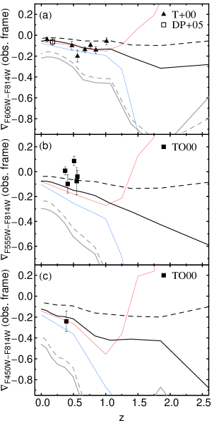
Figure 3: Evolution of observer frame colour gradients and comparison with observations. From top to bottom we plot $\nabla_{\rm F606W-F814W}$, $\nabla_{\rm F555W-F814W}$ and $\nabla_{\rm F450W-F814W}$. The meaning of the curve-styles is as in Fig. 2. The literature data used for the comparison are from Tamura et al. (2000, T+00), De Propris et al. (2005, DP+05) and Tamura & Ohta (2000, TO00). We also plot two toy-models obtained using BC03 synthetic models: 1) the blue line is for the model with a metallicity gradient of $\mbox{$\nabla_{\rm Z}$}\sim-0.4$ constant with redshift and a $z=0$ age gradient of $\mbox{$\nabla_{\rm age}$}\sim 0.04$, 2) the red line is for $\mbox{$\nabla_{\rm Z}$}\sim-0.4$ and a $z=0$ $\mbox{$\nabla_{\rm age}$}\sim-0.04$.

It is now interesting to link the differences found in the gradient normalizations and in the trends with redshift to the initial conditions of the models. In particular, we discuss in the following the relative role of these differences.

• Initial profile. E1 and E3 have a different initial gas profile, IS and flat, respectively. The flat profile in E3 gives shallower gradients and the difference is larger in the external region. Bluer total colours are produced.

• $\rho_{0,gas}$. The role of the central gas density can be analyzed by comparing the predictions for the models E2 and E4. It has a small role in the central regions ($0.1\mbox{$r_{\rm 1/2}$}<r<\mbox{$r_{\rm 1/2}$}$), but in the outer region ($\mbox{$r_{\rm 1/2}$}<r<2\mbox{$r_{\rm 1/2}$}$) it has a strong impact on the gradients, since the smaller central density in E2 produces the positive colour gradients at high redshift and the very flat ones at $z\mathrel{\hbox to0.0pt{\lower 3.5pt\hbox{\hskip 0.5pt$\sim$}\hss}\raise 0.5pt\hbox{$<$}}2$. E2 has also a bluer total colour (bluer than observations). Note that for models E2 and E4 (and similarly for E3), the gas profile is flat, i.e., the gas density is $\rho=\rho_{0,gas}$ everywhere, thus it is not surprising that $\rho_{0,gas}$ affects the outer regions, where it can be immediately consumed to formed stars, more than central ones, where new gas is continuously accreted.

• $\epsilon_{\rm SF}$. E3 and E4 have a different $\epsilon_{\rm SF}$ parameter. In both the regions, the gradients are steeper in E4, thus the higher the SF parameter, the steeper the gradient. From Pipino et al. (2010): basically, an increase in the SF parameter enhances the differences between the inner core and the outskirts set by the other initial conditions.

4 Comparison with observations

We now compare the predictions from our simulations with observations. We have collected several samples ETGs, with stellar masses comparable to ours, at intermediate redshift ($z<1$) and higher redshift ($1<z<2.5$).

• In Sect. 4.1 we start comparing observer frame gradients with low/intermediate redshift galaxies (Tamura et al. 2000; Tamura & Ohta 2000; De Propris et al. 2005).

• In Sect. 4.2 we compare observer- and rest-frame colour gradients with high redshift observations (Guo et al. 2011; Gargiulo et al. 2011, 2012).

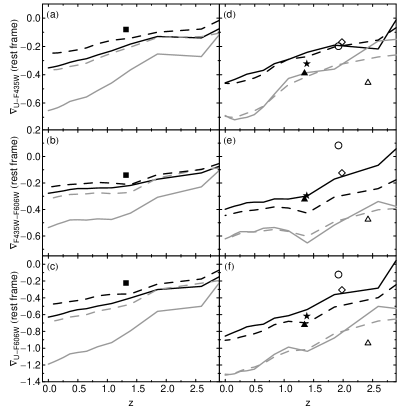
Figure 4: $\nabla_{\rm U-F435W}$, $\nabla_{\rm F435W-F606W}$ and $\nabla_{\rm U-F606W}$ in the rest-frame of the galaxies as a function of redshift. The symbols are as in Figs. 2 and 3. In panels (a), (b) and (c) the gradient is calculated at $r>0.5\,\mbox{$r_{\rm 1/2}$}$, while in panels (d), (e) and (f) at $r>1.5\,\mbox{$r_{\rm 1/2}$}$. The data points are for galaxies in Guo et al. (2011): GOODS IDs 24626 (full box), 19389 (full triangle), 22704 (full star), 23555 (open circle), 24279 (open square) and 23495 (open triangle). For 24626, the authors provide the colour gradients down to $\sim 0.5$ times the effective radius, while for the other galaxies the gradients are calculated down to $\sim 1.5$ times the effective radius. The uncertainties on the gradients are $\sim 0.2$ mag/dex, the error bars are omitted for clarity.

4.1 Low/intermediate redshift observations

Simulations are compared with data at $z<1$ in Fig. 3. In panel (a) we compare the model $\nabla_{\rm F606W-F814W}$ with archival Hubble Deep Field North (HDFN) data of 7 bright ETGs up to $z=1$ from Tamura et al. (2000) and the average gradient (with 1$\sigma$ scatter) of the 22 ETGs in Abell 2218 analyzed in De Propris et al. (2005). We find a fairly good agreement with our E1 model, E3 is consistent with the highest redshift galaxy.

In panel (b) the model $\nabla_{\rm F555W-F814W}$ are compared with gradients for ETGs in 5 clusters at redshifts $z=0.37-0.56$ ($\rm A370$, $\rm CL\,0939+47$, $\rm CL\,0412-65$, $\rm CL\,0016+16$ and $\rm CL\,0054-27$) with measured photometry in F555W and F814W band passes. The average gradients with $1\sigma$ scatter in each cluster are plotted. The agreement is worse with E1 except for $\rm CL0939+47$ and data seem to better agree with E3.

In panel (c) the model $\nabla_{\rm F450W-F814W}$ are compared with the mean gradients for ETGs in $\rm CL0024+16$ analyzed in Tamura & Ohta (2000). Here the agreement with E1 is very good.

In general, $z<1$ data seem to favor models where the gradient is shallow, close to $z\sim 0$ values, without strong signs of evolution. This is not entirely surprising, if one sets the formation of ETGs at $z>2$ with passively evolving galaxies already at $z\sim 2$. However, half of our models (i.e. E2 and E4), despite the high formation redshift and the passive evolution, still predict a strong evolution of the color gradients (see the strong rest-frame evolution in Fig. 2).

To ease the comparison between such observations and model predictions in Fig. 3 we have also plotted two toy-model galaxies adopting the BC03 SPS, with negative metallicity gradient of $\mbox{$\nabla_{\rm Z}$}\sim-0.4$, and small positive (negative) age gradients of $\mbox{$\nabla_{\rm age}$}\sim 0.04$ ($\mbox{$\nabla_{\rm age}$}\sim-0.04$) at $z=0$. In these models, the $\nabla_{\rm Z}$ is constant as a function of redshift (since the Z is fixed in the BC03 models), while $\nabla_{\rm age}$ is changing, getting steeper and steeper at higher redshift. Following the redshift evolution we notice that the two toy-models reproduce fairly well observations at $z<1$ (consistently with our monolithic predictions).

Thus, we have shown that the SP gradients predicted by our models (for instance E1 and E3, i.e. with final $\mbox{$\nabla_{\rm Z}$}\sim-0.2$ and $\mbox{$\nabla_{\rm age}$}\sim 0$) reproduce local and $z<1$ observations. Consistently with the toy-models plotted in Fig. 3 our conclusions are in agreement with Tamura et al. (2000) and Tamura & Ohta (2000), which have demonstrated that metallicity gradients alone do reproduce the observed colour gradients (with null age gradients), whereas age gradient alone do not.

4.2 High redshift observations

A larger scatter in the color gradients is, instead, expected at $z>1$, when we approach the epoch of formation of the galaxies and even a small scatter in their assembly redshift, or the earlier phases of passive evolution, may enhance the radial differences in the SP properties.

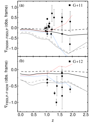
Figure 5: The same as Fig. 3. From top to bottom we plot $\nabla_{\rm F606W-F850LP}$ and $\nabla_{\rm F850LP-F160W}$. The literature data used for the comparison are from Gargiulo et al. (2011, G+11) and Gargiulo et al. (2012, G+12). The style of the curves and toy-models are as in Fig. 3.

In Fig. 4 we compare our predictions with rest-frame colours from Guo et al. (2011). Guo et al. (2011) have analyzed the properties of six massive galaxies (with masses in the range $\sim 1.5-13\times 10^{10}\,\mbox{$M_{\odot}$}$, assuming a Salpeter IMF) from the GOODS south field in VIMOS-VLT U-band, and HST F435W- and F606W-bands. They have first converted their data to rest-frame quantities, measuring gradients from $\sim 1.5$ to $\sim 8$ times the H-band effective radius, and in one case (ID 24626) they were able to follow the gradients down to $\sim 0.5$ times the effective radius. To homogenously compare with these data, in Fig. 4 we calculate the gradients from $0.5$ (left panels) and $1.5$ (right panels) times the $r_{\rm 1/2}$ of the model galaxy. Although such observations have been converted to rest-frame quantities, introducing further uncertainty to the comparison, we find an excellent agreement with our set of models, with only a couple of outliers.

Moreover, in Fig. 5 the model predictions for $\nabla_{\rm F606W-F850LP}$ and $\nabla_{\rm F850LP-F160W}$ are compared with the results for ETGs at $1<z<2$ selected from the GOODS-South field and analyzed in Gargiulo et al. (2011) and Gargiulo et al. (2012), respectively. These galaxies are selected on the basis of a visual inspection of F850LP images and of the Sérsic index, $n_{\rm F850LP}$ ($n_{\rm F850LP}>2$), and span a range of masses $\sim(3-50)\times 10^{10}\,\rm\mbox{$M_{\odot}$}$ (Salpeter IMF). From the panel (a), within the data and simulation uncertainties E1 and E3 are quite consistent with a large fraction of the ETGs. Unfortunately, our simulations are not able to reproduce the positive $\nabla_{\rm F606W-F850LP}$ found in some of the galaxies, since negative $\nabla_{\rm Z}$ and negligible $\nabla_{\rm age}$ are produced at all the epochs (see Table 1). On the contrary, from the panel (b), few datapoints agree with E1 and E3 within uncertainties, some other galaxies are in better agreement with E2 and E4 and few other ones have quite steep gradients the models do not reproduce.

In Fig. 5 we have also plotted the two toy-model galaxies first shown in Fig. 3. At $z~{}\hbox to0.0pt{$>$\hss}{\lower 4.30554pt\hbox{$\sim$}}1$, the strongest (with respect to $z<1$) positive and negative $\nabla_{\rm age}$ produce a strong evolution of colour gradients. A discrepancy emerges from these results, since strong positive $\nabla_{\rm age}$ at large redshifts fit the positive $F666W-F850LP$ gradients found in Gargiulo et al. (2011, panel (a)), while a negative $\nabla_{\rm age}$ would reproduce the steep negative $F850LP-F160W$ gradients in Gargiulo et al. (2012, panel (b)).

4.3 Systematics and missing ingredients

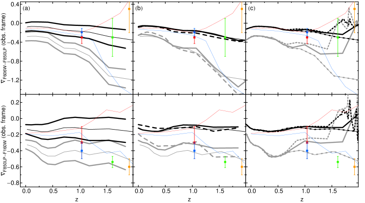
Figure 6: Systematics in observer frame colour gradients. $\nabla_{\rm F606W-F850LP}$ (top panels) and $\nabla_{\rm F850LP-F160W}$ (bottom panels) for E1 (black lines) and E4 (gray lines) are plotted as a function of z. The reference model is plotted as thin line. From the left to the right we show: (a) the role of positive and negative gradients in the extinction (which bracket the case with no dust extinction); (b) the role of SPS prescription, BC03 is compared with BC03-updated (thick line) and M05 (dashed thick line); (c) the impact of a change of the formation redshift: $z_{\rm f}=2.5$ (thick line), $2$ (short dashed thick line) and $6$ (long dashed thick line); see text for further details. The red and blue lines are the same toy-models plotted in Figs. 3 and 5. The colored boxes and bars are for the four galaxies shared by Gargiulo et al. (2011) and Gargiulo et al. (2012): IDs 23 (red), 11888 (blue), 2111 (green) and 472 (orange).

In order to investigate further the discrepancies discussed above we have:

• analyzed the impact of some ingredients, (as dust extinction, SPS prescription and formation redshift) on our results, and

• performed a more detailed comparison with high-redshift observations, picking those galaxies in common between the two papers (Gargiulo et al. 2011, 2012), having both $F666W-F850LP$ and $F850LP-F160W$ measured (i.e. the galaxies with IDs 23, 11888, 2111 and 47; see the papers above for further details).

4.3.1 Systematics

We start by analyzing the role of dust extinction, SPS prescription and formation redshift on our results in Fig. 6. For sake of clarity we only limit the analysis to the models E1 and E4.

We first show in panels (a) the role of dust extinction. We adopt the extinction law from Cardelli et al. (1989) with $R_{V}=3.1$, calculating the corrections to the observer-frame colours and the relative colour gradients. Due to our ignorance about dust gradients in high redshift galaxies, we will rely on the simplest hypothesis, we will assume a dust extinction gradient of $\nabla E(B-V)=\pm 0.2$ constant with redshift. The impact on the gradients is of $\pm 0.1$, a steeper (shallower) negative gradient corresponds to the model with a larger (smaller) fraction of dust in the center.

In panels (b) we show that the use of either the BC03-updated prescription (Eminian et al. 2008) or the M05 models leaves almost unchanged the optical colour gradient, while can provide shallower near-IR gradients.

The effect of the change in the formation redshift is shown in panels (c), where we notice that smaller formation redshifts (e.g. $z_{\rm f}=2$ and $2.5$) give shallower colour gradients at $z~{}\hbox to0.0pt{$>$\hss}{\lower 4.30554pt\hbox{$\sim$}}0.5$ and positive at $z~{}\hbox to0.0pt{$>$\hss}{\lower 4.30554pt\hbox{$\sim$}}1.5$.

4.3.2 Understanding the discrepancies with high-z ETGs

In Fig. 6 we also plot the four galaxies shared by Gargiulo et al. (2011) and Gargiulo et al. (2012). The galaxy with ID 23 agrees with E1, within statistical uncertainties. This agreement improves if we have more dust in the center than in the peripheries, making the gradients slightly steeper. If we consider more dust in the peripheries the galaxy also matches the results from E4. However, this scenario seems not plausible (Gargiulo et al. 2012). The agreement with E4 can be improved if we assume a smaller $z_{\rm f}$ for our model. Consistently with our models, a synthetic toy-model with a suitable negative $\nabla_{\rm Z}$ and a mild (positive or negative) age gradients can also reproduce the observations for this galaxy (see also Fig. 3). For the other galaxies (IDs 11888, 2111, 472) no agreement can be found with our models and synthetic toy-models explored. The situation gets worse for galaxies 2111 and 472. These systems are characterized by null or positive $\nabla_{\rm F606W-F850LP}$ and steep negative $\nabla_{\rm F850LP-F160W}$, which cannot be accounted by our models, and nor by any combination of $\nabla_{\rm age}$, $\nabla_{\rm Z}$, gradients in the dust extinction, a change in $z_{\rm f}$. As a confirmation of our results, by means of a SPS analysis Gargiulo et al. (2012) reach similar conclusions, suggesting the simultaneous variation of several parameters (e.g., age, Z, SF duration, IMF slope, dust extinction, etc.), which will require further analysis.

5 Physical scenario

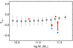
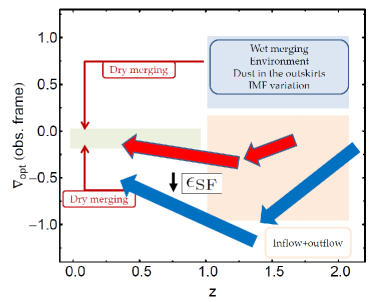
Figure 7: Top panel. $\nabla_{\rm g-i}$ as a function of stellar mass. We plot the $z=0$ gradients for E1 (red open box), E2 (blue filled triangle), E3 (red filled box) and E4 (blue filled box). The black open boxes and error bars are for medians and 25-75th quantiles of results for local SDSS ETGs in Tortora et al. (2010). The red vertical arrows show a qualitative impact of dry mergings on the model gradients. Bottom panel. Optical colour vs redshift in the observer frame. The shaded rectangles set the regions on the plane where observations fall. The red and blue arrows give a qualitative view of the trends of our models (red arrows for E1 and E2; blue arrows for E2 and E4) as shown, for instance, more quantitatively in Figs. 3 and 5. The black small arrow show how an increase of SF parameter affects gradients. Information about the physical processes involved are also shown. See the text for a full discussion of this picture.

We finally gain insights on the physical processes or any missing ingredients in our analysis. The general physical picture is given in the bottom panel of Fig. 7. We have shown that, although there are some disagreements with some high redshift observations (e.g. Gargiulo et al. 2011, 2012), our monolithic models can reproduce a wide collection of low/intermediate redshift data samples and a fraction of data at high redshift (e.g. Tamura et al. 2000; Tamura et al. 2000; De Propris et al. 2005; Guo et al. 2011). The interplay between the evolution of the metallicity profiles and the radial behaviour of the SF history, both combined via the SPS prescription, drives the evolution of the optical and near-IR colours. Stars in all models are formed at very early stages ($z_{\rm f}~{}\hbox to0.0pt{$>$\hss}{\lower 4.30554pt\hbox{$\sim$}}4$) and in a short period, in agreement with previous literature (Matteucci 1994; Thomas et al. 2005), while at later stages the galaxies evolve passively. The optical colours typically show stronger redshift evolution during this passive phase when compared with the near-IR one. In the early stages the models also present some strong features and very strong negative colour gradients.

Thus, accordingly to other sets of observables (as metallicity and $[\alpha/Fe]$), a wide range of observations can be reproduced by the interplay of gas infall and outflow from evolved stars and supernovae. In particular, while the models with a smaller $\epsilon_{\rm SF}$ can consistently reproduce the data at $z\mathrel{\hbox to0.0pt{\lower 3.5pt\hbox{\hskip 0.5pt$\sim$}\hss}\raise 0.5pt\hbox{$<$}}1$ (Tamura et al. 2000; Tamura et al. 2000; De Propris et al. 2005) and local observations (see top panel in Fig. 7; Tortora et al. 2010), those with larger $\epsilon_{\rm SF}$ produce colour gradients which are steeper than local observations. To reconcile the latter models with results at $z\mathrel{\hbox to0.0pt{\lower 3.5pt\hbox{\hskip 0.5pt$\sim$}\hss}\raise 0.5pt\hbox{$<$}}1$ further physical ingredients are necessary. The occurrence of at least one dry major merger at $z\mathrel{\hbox to0.0pt{\lower 3.5pt\hbox{\hskip 0.5pt$\sim$}\hss}\raise 0.5pt\hbox{$<$}}1$ (Di Matteo et al. 2009) could wash out the gradients from the latter models (E2 and E4) producing shallower gradients which are consistent with local estimates (see top panel in Fig. 7; Kobayashi 2004) and reproducing quite well all the other local correlations, but the occurrence of such events seem relatively uncommon (De Propris et al. 2010).

Our models have been built to reproduce the local negative metallicity gradients at low redshift and do not predict positive observer-frame $\nabla_{\rm F606W-F850LP}$ at high redshift (jointly with the negative $\nabla_{\rm F850LP-F160W}$). Such positive gradients, although not common in the local massive ETGs, are found at higher redshift (e.g. Menanteau et al. 2001; Ferreras et al. 2009; Gargiulo et al. 2011). They can be possibly reconciled with the simulated negative gradients if we assume a) they have a huge amount of dust in the external regions ($\nabla E(B-V)>0.2$; Fig. 6), and/or b) interactions with environment have stripped off the outer gas, and/or c) a wet merging has generated a starburst in the core (Hopkins et al. 2009), and/or d) a change of IMF with radius inducing positive colour gradients (Gargiulo et al. 2012). Subsequent dry mergings could wash out such gradients contributing to match the local observations. If on the one hand too strong gradients in the dust seem unrealistic, our models are built for isolated galaxies, and do not take into account exogen phenomena as merging/close encounters/etc. or any variation in the IMF, which could make redder the outskirts and the observed gradients positive. However, it seems not realistic to reproduce some gradients observed (Gargiulo et al. 2011, 2012) with any combination of age, metallicity and dust extinction (see Fig. 6). Further physical “unexplored” galactic ingredients accounting for such features need to be investigated. Recently, many works have contrasted the IMF universality, suggesting a systematic IMF variation with mass (Conroy & van Dokkum 2012; Cappellari et al. 2012b; Tortora et al. 2012; Ferreras et al. 2012; Tortora et al. 2013) and with redshift (van Dokkum 2008). It is likely that IMF can change as a function of redshift and within each galaxy, inducing non trivial variations in colour gradients (Gargiulo et al. 2012).

6 Conclusions

We have adopted monolithic hydrodynamical models of four massive ETGs (which we have called E1, E2, E3 and E4) from Pipino et al. (2008), which are combined with SPS models from Bruzual & Charlot (2003) to convert the simulated metallicities and SF history into observed quantities as colour gradients. Therefore, we provide a suite of model predictions which can be directly compared with low/high redshift measurements (without any intermediate step, as the SPS fitting to derive age/metallicity gradients in measured colour gradients). So far the new monolithic models proposed and analyzed in Pipino et al. (2008) and Pipino et al. (2010) – characterized by two main contrasting phenomena, infall of gas from the outer regions, and outflows due to the stellar and SN winds – reproduce some global correlations in local galaxies, as the Z- and $[\alpha/Fe]$-mass relations and give shallower $\nabla_{\rm Z}$ with respect to earlier models (e.g. Larson 1974; Carlberg 1984). In particular, Pipino et al. (2010) have demonstrated that the models reproduce fairly well a) the average Z gradients ($\mbox{$\nabla_{\rm Z}$}\sim-0.3$) and b) the observed scatter in local ETGs. This improvement of the models has been possible thanks to the requirement, matched by the models, that the stars produced have high average $[\alpha/Fe]$ in the cores and thus short SF (as found by observations; Matteucci 1994; Thomas et al. 2005; Tortora et al. 2009b) and smaller age gradients (Tortora et al. 2010). The aim of the present paper has consisted to present the redshift evolution of the color gradient in the simulated galaxies and to further constrain the model parameters by means of new and independent dataset. From the comparison with data, we infer the following main conclusions:

• The models E1 and E3 show a quite good agreement with data sets at $z\simeq 0$ (local SDSS galaxies from Tortora et al. (2010) - the top panel of Fig. 7), $z\mathrel{\hbox to0.0pt{\lower 3.5pt\hbox{\hskip 0.5pt$\sim$}\hss}\raise 0.5pt\hbox{$<$}}1$ (Fig. 6; Tamura et al. 2000; Tamura & Ohta 2000; De Propris et al. 2005) as well as with the rest-frame colour gradients derived in Guo et al. (2011) for a sample of six high-redshift ($z>1$) galaxies.

  As already pointed out in Pipino et al. (2010) (for the intrinsic metallicity gradients) the higher is the SF parameter, the steeper the color gradient. Since the observations agree with those models with shallower gradients (E1 and E3), the data-model comparison seems to favor small values for $\epsilon_{\rm SF}$.

• Despite the previous encouraging results, some disagreement is found when we further add the high redshift galaxies by Gargiulo et al. 2011, 2012. In particular, we find that the optical data tend to favor models producing the shallower colour and metallicity gradients (i.e. E1 and E3), while most of the near-infrared gradients are consistent with the models with steeper gradients (i.e. E2 and E4).

• Assuming that this latter case is true, models with higher $\epsilon_{\rm SF}$ would require the intervention of some process which flatten the gradients, as, at least, 1 dry merger at $z\mathrel{\hbox to0.0pt{\lower 3.5pt\hbox{\hskip 0.5pt$\sim$}\hss}\raise 0.5pt\hbox{$<$}}1$ to match local observations.

• Models allow us to investigate the role of other physical processes, parameterized through different initial conditions, as the central gas density, the gas density distribution. Their effect on the gradient is smaller than that of $\epsilon_{\rm SF}$, therefore, we present predictions that can be constrained when the statistics on high redshift gradients improve. In particular, when the initial gas distribution is flat, then the colour gradients are shallower and the difference is stronger in the outer regions. A smaller gas density, as in the model E2 will give slightly shallower colour gradients in the central regions ($0.1\mbox{$r_{\rm 1/2}$}<r<\mbox{$r_{\rm 1/2}$}$), while positive (at $z~{}\hbox to0.0pt{$>$\hss}{\lower 4.30554pt\hbox{$\sim$}}1.5$) or null (at $z\mathrel{\hbox to0.0pt{\lower 3.5pt\hbox{\hskip 0.5pt$\sim$}\hss}\raise 0.5pt\hbox{$<$}}1.5$) in the outer region ($\mbox{$r_{\rm 1/2}$}<r<2\mbox{$r_{\rm 1/2}$}$).

• To further investigate the inconsistency among the data in Gargiulo et al. (2011) and Gargiulo et al. (2012) we have picked out the four galaxies with both the F606W-F850LP and F850LP-F160W colours measured, and we find that our models can reproduce consistently only one of the selected galaxies, having some troubles to fit the others. Gargiulo et al. (2012) have pointed out that the variation of a single SP parameter is not able to reproduce the observed colour gradients and global SED. This would suggest that a simultaneous variation of several parameters has to be invoked to reproduce such a data. Unfortunately, we have verified that, not only our models do not work, but, using SPS toy-models, combinations of age and metallicity gradients fail to reproduce such observations. Some further parameter or more complex phenomena would be taken into account to reproduce such observations.

We have finally discussed our results within a more complex physical scenario (see Sect. 5). As we have amply discussed, although our models reproduce several observational data, seem to fail in some galaxies at $1<z<2$. In particular, our models, by construction, do not reproduce the steep positive optical colour gradients ($\nabla_{\rm F606W-F850LP}$) in Gargiulo et al. (2011), which can be possibly originated by a) wet mergings, b) interaction with environment, c) strong dust extinction gradients or d) IMF variation across the galaxies. Moreover, the unsuccessful matching of combined data from Gargiulo et al. (2011) and Gargiulo et al. (2012) seem to be a difficult task to achieve adopting combinations of gradients in age, metallicity and dust extinction, suggesting that more work is needed to reproduce observations, including further and unexplored ingredients in the simulations. Larger observational samples of gradients in high-redshift ETGs (out to one effective radius and beyond) can confirm the results discussed in this paper, validating the models or suggesting the intervention of further physical processes, as (dry or wet) galaxy mergings, environmental phenomena, AGN feedback or questioning the assumptions about stellar ingredients, as the IMF universality suggesting possible variations in terms of the galactocentric radius (Tortora et al. 2013).

References

- Annibali et al. (2007) Annibali F., Bressan A., Rampazzo R., Zeilinger W. W., Danese L., 2007, A&A, 463, 455
- Bedogni & D’Ercole (1986) Bedogni R., D’Ercole A., 1986, A&A, 157, 101
- Bekki & Shioya (1999) Bekki K., Shioya Y., 1999, ApJ, 513, 108
- Bruzual & Charlot (2003) Bruzual G., Charlot S., 2003, MNRAS, 344, 1000
- Cappellari et al. (2012a) Cappellari M. et al., 2012a, Nature, 484, 485
- Cappellari et al. (2012b) Cappellari M. et al., 2012b, MNRAS, submitted, arXiv:1208.3523
- Cardelli et al. (1989) Cardelli J. A., Clayton G. C., Mathis J. S., 1989, ApJ, 345, 245
- Carlberg (1984) Carlberg R. G., 1984, ApJ, 286, 403
- Carollo et al. (1993) Carollo C. M., Danziger I. J., Buson L., 1993, MNRAS, 265, 553
- Colavitti et al. (2009) Colavitti E., Pipino A., Matteucci F., 2009, A&A, 499, 409
- Conroy & van Dokkum (2012) Conroy C., van Dokkum P., 2012, ApJ, in press, arXiv:1205.6473
- Davies et al. (1993) Davies R. L., Sadler E. M., Peletier R. F., 1993, MNRAS, 262, 650
- De Lucia et al. (2006) De Lucia G., Springel V., White S. D. M., Croton D., Kauffmann G., 2006, MNRAS, 366, 499
- De Propris et al. (2005) De Propris R., Colless M., Driver S. P., Pracy M. B., Couch W. J., 2005, MNRAS, 357, 590
- De Propris et al. (2010) De Propris R. et al., 2010, AJ, 139, 794
- Di Matteo et al. (2009) Di Matteo P., Pipino A., Lehnert M. D., Combes F., Semelin B., 2009, A&A, 499, 427
- Eminian et al. (2008) Eminian C., Kauffmann G., Charlot S., Wild V., Bruzual G., Rettura A., Loveday J., 2008, MNRAS, 384, 930
- Ferreras et al. (2012) Ferreras I., La Barbera F., de Carvalho R. R., de la Rosa I. G., Vazdekis A., Falcon-Barroso J., Ricciardelli E., 2012, MNRAS, in press, arXiv:1204.3823
- Ferreras et al. (2009) Ferreras I., Lisker T., Pasquali A., Kaviraj S., 2009, MNRAS, 395, 554
- Gargiulo et al. (2011) Gargiulo A., Saracco P., Longhetti M., 2011, MNRAS, 412, 1804
- Gargiulo et al. (2012) Gargiulo A., Saracco P., Longhetti M., La Barbera F., Tamburri S., 2012, MNRAS, 425, 2698
- Guo et al. (2011) Guo Y. et al., 2011, ApJ, 735, 18
- Hopkins et al. (2009) Hopkins P. F., Cox T. J., Dutta S. N., Hernquist L., Kormendy J., Lauer T. R., 2009, ApJS, 181, 135
- Kawata (2001) Kawata D., 2001, ApJ, 558, 598
- Kobayashi (2004) Kobayashi C., 2004, MNRAS, 347, 740
- Kroupa (2001) Kroupa P., 2001, MNRAS, 322, 231
- Kuntschner et al. (2006) Kuntschner H. et al., 2006, MNRAS, 369, 497
- Kuntschner et al. (2010) Kuntschner H. et al., 2010, MNRAS, 408, 97
- La Barbera et al. (2011) La Barbera F., Ferreras I., de Carvalho R. R., Lopes P. A. A., Pasquali A., de la Rosa I. G., De Lucia G., 2011, ApJ, 740, L41
- La Barbera et al. (2004) La Barbera F., Merluzzi P., Busarello G., Massarotti M., Mercurio A., 2004, A&A, 425, 797
- Larson (1974) Larson R. B., 1974, MNRAS, 166, 585
- Maraston (2005) Maraston C., 2005, MNRAS, 362, 799
- Martinelli et al. (1998) Martinelli A., Matteucci F., Colafrancesco S., 1998, MNRAS, 298, 42
- Matteucci (1994) Matteucci F., 1994, A&A, 288, 57
- McCarthy et al. (2007) McCarthy I. G., Bower R. G., Balogh M. L., 2007, MNRAS, 377, 1457
- Menanteau et al. (2001) Menanteau F., Jimenez R., Matteucci F., 2001, ApJ, 562, L23
- Ogando et al. (2005) Ogando R. L. C., Maia M. A. G., Chiappini C., Pellegrini P. S., Schiavon R. P., da Costa L. N., 2005, ApJ, 632, L61
- Pipino et al. (2010) Pipino A., D’Ercole A., Chiappini C., Matteucci F., 2010, MNRAS, 407, 1347
- Pipino et al. (2008) Pipino A., D’Ercole A., Matteucci F., 2008, A&A, 484, 679
- Pipino et al. (2009) Pipino A., Devriendt J. E. G., Thomas D., Silk J., Kaviraj S., 2009, A&A, 505, 1075
- Pipino & Matteucci (2004) Pipino A., Matteucci F., 2004, MNRAS, 347, 968
- Pipino et al. (2002) Pipino A., Matteucci F., Borgani S., Biviano A., 2002, New A, 7, 227
- Rawle et al. (2010) Rawle T. D., Smith R. J., Lucey J. R., 2010, MNRAS, 401, 852
- Romeo et al. (2008) Romeo A. D., Napolitano N. R., Covone G., Sommer-Larsen J., Antonuccio-Delogu V., Capaccioli M., 2008, MNRAS, 389, 13
- Salpeter (1955) Salpeter E. E., 1955, ApJ, 121, 161
- Sánchez-Blázquez et al. (2007) Sánchez-Blázquez P., Forbes D. A., Strader J., Brodie J., Proctor R., 2007, MNRAS, 377, 759
- Sánchez-Blázquez et al. (2006) Sánchez-Blázquez P., Gorgas J., Cardiel N., 2006, A&A, 457, 823
- Scott et al. (2009) Scott N. et al., 2009, MNRAS, 398, 1835
- Silich & Tenorio-Tagle (1998) Silich S. A., Tenorio-Tagle G., 1998, MNRAS, 299, 249
- Spolaor et al. (2010) Spolaor M., Kobayashi C., Forbes D. A., Couch W. J., Hau G. K. T., 2010, MNRAS, 408, 272
- Spolaor et al. (2009) Spolaor M., Proctor R. N., Forbes D. A., Couch W. J., 2009, ApJ, 691, L138
- Tamura et al. (2000) Tamura N., Kobayashi C., Arimoto N., Kodama T., Ohta K., 2000, AJ, 119, 2134
- Tamura & Ohta (2000) Tamura N., Ohta K., 2000, AJ, 120, 533
- Thomas et al. (2005) Thomas D., Maraston C., Bender R., Mendes de Oliveira C., 2005, ApJ, 621, 673
- Thomas et al. (2007) Thomas D., Maraston C., Schawinski K., Sarzi M., Joo S.-J., Kaviraj S., Yi S. K., 2007, in IAU Symposium, Vol. 241, IAU Symposium, Vazdekis A., Peletier R., eds., pp. 546–550
- Thornton et al. (1998) Thornton K., Gaudlitz M., Janka H.-T., Steinmetz M., 1998, ApJ, 500, 95
- Tortora et al. (2009a) Tortora C., Antonuccio-Delogu V., Kaviraj S., Silk J., Romeo A. D., Becciani U., 2009a, MNRAS, 396, 61
- Tortora et al. (2012) Tortora C., La Barbera F., Napolitano N. R., de Carvalho R. R., Romanowsky A. J., 2012, MNRAS, 425, 577
- Tortora et al. (2010) Tortora C., Napolitano N. R., Cardone V. F., Capaccioli M., Jetzer P., Molinaro R., 2010, MNRAS, 407, 144
- Tortora et al. (2009b) Tortora C., Napolitano N. R., Romanowsky A. J., Capaccioli M., Covone G., 2009b, MNRAS, 396, 1132
- Tortora et al. (2013) Tortora C., Romanowsky A. J., Napolitano N. R., 2013, ApJ, 765, 8
- Tortora et al. (2011) Tortora C., Romeo A. D., Napolitano N. R., Antonuccio-Delogu V., Meza A., Sommer-Larsen J., Capaccioli M., 2011, MNRAS, 411, 627
- Treu et al. (2010) Treu T., Auger M. W., Koopmans L. V. E., Gavazzi R., Marshall P. J., Bolton A. S., 2010, ApJ, 709, 1195
- van Dokkum (2008) van Dokkum P. G., 2008, ApJ, 674, 29
- Welikala & Kneib (2012) Welikala N., Kneib J.-P., 2012, ArXiv e-prints