The stellar metallicity distribution of the Milky Way from the BATC survey

Abstract

Using the stellar atmospheric parameters such as effective temperature and metallicity derived from SDSS spectra for $\sim 2200$ main sequence (MS) stars which were also observed by Beijing - Arizona - Taiwan - Connecticut (BATC) photometric system, we develop the polynomial photometric calibration method to evaluate the stellar effective temperature and metallicity for BATC multi-color photometric data. This calibration method has been applied to about 160 000 MS stars from 67 BATC observed fields. Those stars have colors and magnitudes in the ranges $0.1<d-h<1.4$ and $14.0\leq d<21.0$. We find that there is a peak of metallicity distribution at $\rm{[Fe/H]}\sim-1.5$ in the distance from the Galactic plane $|Z|>5~{}\rm{kpc}$ which corresponds to the halo component and a peak at $\rm{[Fe/H]}\sim-0.7$ in the region 2 $<|Z|\leqslant 5~{}\rm{kpc}$ where is dominated by the thick disk stars. The mean stellar metallicity smoothly decreases from $-0.65$ to $-0.78$ in the interval $0.5<|Z|\leqslant 2~{}\rm{kpc}$. Metallicity distributions in the halo and the thick disk seem invariant with the distance from the Galactic plane.

1 INTRODUCTION

Studies of the Galactic stellar chemical distribution are imperative for the Galaxy formation and evolution. The metal-poor end of the metallicity distribution function reveals information about the early era of star formation in the Galaxy, while the metal-rich end of the metallicity distribution function reflects recent Galaxy conditions (Schwarzschild et al., 1955). There is a wide range of Galaxy formation models corresponding to different predications about the stellar metallicity distribution. Eggen et al. (1962) provided a steady Galaxy formation scenario, ELS model. At the beginning of the Galaxy formation, a relatively rapid radical collapse of the initial protogalactic cloud happened, followed by the equally rapid setting of gas into rotating disk. A steady process of the Galaxy formation leads to smooth distribution of stars. However, recent discoveries of complex substructure conflict with the simple collapse model. Many irregular substructures such as Sagittarius dwarf tidal stream (Ivezić et al., 2000; Yanny et al., 2000; Vivas et al., 2001; Majewski et al., 2003), Virgo Stellar Stream (Duffau et al., 2006; Prior et al., 2009) and the Monoceros stream closer to the Galactic plane (Newberg et al., 2002; Rocha-Pintoet al., 2003) were found in the recent large area sky surveys. Recent observations show that the Galactic structure is a complex and dynamic structure. The SZ model that the Galaxy formed at least partly through the merge of larger systems was advanced by Searle & Zinn (1978). This hypothesis is supported by recent studies of stellar kinematics and metallicity distribution (Majewski et al., 1996; Belokurov et al., 2006; Jurić et al., 2008).

The metallicity distribution of different Galactic components can be used to constrain the Galaxy formation and evolution models. The thin disk, the thick disk and the halo are the basic components of the Galaxy. Stars on more radial orbits are metal-poor than stars on planar orbits. This conclusion is supported by the observation data (Bahcall & Soneira, 1980; Gilmore & Reid, 1983; Gilmore et al., 1989). The ELS model cannot explain the Galaxy halo without metallicity gradient while the SZ model is able to account for the lack of metallicity gradient of the halo. Different thick disk formation scenarios correspond to different abundance distribution in the thick disk. If the thick disk was formed in the Galaxy collapse, there must be a stellar metallicity gradient in the thick disk. Chen et al. (2011) found that a vertical gradient of $-0.22\pm 0.07$ dex $\rm{kpc^{-1}}$ for the thick disk. On the other hand, the absence of the stellar metallicity gradient in the thick disk favor the thick disk was formed through merger of larger system or via kinematic heating of the thin disk. There has been much debate about the thick disk, some researchers pointed out that the two components of disk cannot be separable from one another (Norris & Ryan, 1991; Bovy et al., 2012). Ivezić et al. (2008) suggested that the metallicity and velocity distribution of the disk can be described by a single disk component instead of two separate ones.

The most precise methods to derive the stellar metallicity are based on the spectroscopic survey (Allende et al., 2006; Ivezić et al., 2012). However, imaging survey data provide better sky and depth coverage than spectroscopic survey data. The photometric metallicity methods are based on the theory that the density of metallicity absorption lines is highest in the blue spectral region. Low metal abundance produces weak atmospheric absorption lines and increased ultraviolet emission (Schwarzschild et al., 1955; Sandage, 1969; Beers & Christlieb, 2005). Siegel et al. (2009) derived approximate stellar abundance through measurement of ultraviolet excess, despite this method is less precise in larger distance. Ivezić et al. (2008) demonstrated that for the MS stars, the stellar metallicity estimate can be derived through SDSS color indices. This calibration of the metallicity has been applied for millions of stars to explore the metallicity distribution of the Galaxy. In this paper, we present an analysis of stars in the BATC photometric survey. Some Galactic structure and stellar metallicity distribution studies have been carried out using the BATC photometric data (Du et al., 2003, 2004, 2006; Peng et al., 2012). Peng et al. (2012) adopted the spectral energy distribution (SED) fitting method to evaluate the stellar metallicity in the Galaxy. With the new metallicity calibration method and more BATC photometric survey fields used in this paper, it is possible to derive more information about the stellar metallicity distribution of the Galaxy.

In this paper, we attempt to study the Galactic stellar metallicity distribution using photometric metallicity method. In total, there are 67 BATC photometric survey fields used in this paper. Section 2 of this paper describes the way to select star sample. The methods of stellar atmospheric parameters estimation are described in Section 3. The stellar metallicity distribution is discussed in Section 4. Finally, in Section 5, we summarize our main conclusions in this study.

2 OBSERVATIONS AND DATA

2.1 BATC survey and data reduction

The BATC photometric survey is carried out by the BATC multi-color system with the 60/90 cm f/3 Schmidt telescope at the Xinglong station, National Astronomical Observatories of Chinese Academy of Sciences (NAOC). A Ford 4096 $\times$ 4096 CCD camera was equipped at the prime focus of the telescope. The field of view is 92 $\times$ 92 arcmin² with a spatial scale of 1.36 arcsec pixel^-1. The BATC system contains 15 intermediate-band filters, covering a wavelength from 3000 to 10 000 Å which are designed to avoid strong night-sky emission lines (Fan et al., 1996). The parameters of the BATC filters are listed in Table 1. Col. (1) and Col. (2) represent the ID of the BATC filters, Col. (3) and Col. (4) represent the central wavelengths and FWHM of the 15 filters, respectively (Peng et al., 2012). Using automatic data-processing software, PIPELINE I (Fan et al., 1996), we carry out the standard procedures of bias subtraction and flat-field correction. The PIPELINE II reduction procedure is performed on each single CCD frame to get the point spread function (PSF) magnitude of each point source (Zhou et al., 2003). The BATC magnitude adopt the monochromatic AB magnitude as defined by Oke & Gunn (1983). The detailed description of the BATC photometric system and flux calibration of the standard stars can be found in Fan et al. (1996) and Zhou et al. (2003).

Table 1: Parameters of the BATC filters

No.	Filter	Wavelength	FWHM
		(Å)	(Å)
1	$a$	3371.5	359
2	$b$	3906.9	291
3	$c$	4193.5	309
4	$d$	4540.0	332
5	$e$	4925.0	374
6	$f$	5266.8	344
7	$g$	5789.9	289
8	$h$	6073.9	308
9	$i$	6655.9	491
10	$j$	7057.4	238
11	$k$	7546.3	192
12	$m$	8023.2	255
13	$n$	8484.3	167
14	$o$	9182.2	247
15	$p$	9738.5	275

Accurate determination of the properties of the components of the Galaxy requires surveys with sufficient sky coverage to assess the overall geometry (de Jong et al., 2010). Most previous investigations about the Galactic metallicity distribution used only one or a few fields along the lines-of-sight (Du et al., 2004; Siegel et al., 2009; Karatas et al., 2009). The fields used in this paper are toward different directions, the Galactic center, the anticentre at median and high latitudes, $20^{\circ}<|b|<60^{\circ}$. We try to choose the MS stars to carry out our study. The distribution of all stars in the BATC d filter in the BATC T192 and T193 fields is shown in Figure 1. Owing to the BATC observing strategy, stars brighter than $d=14$ mag are saturated. In addition, from Figure 1, we can see that star counts are not completed for magnitudes fainter than $d=21.0$ mag. So our work is restricted to the magnitude range $14\leqslant d<21$. The MS stars with colors located in the proper range for application the photometric metallicity method are needed. The specifical criteria used to choose MS stars are the following:

1. $14\leq d<21$;

2. $0.1<(d-h)<1.4$;

3. $0<(d-n)<2.5$;

4. $-0.7<(d-n)-1.6(d-h)<0.8$.

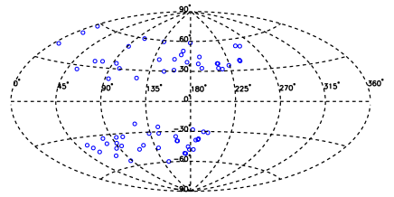
Figure 3: The Galactic longitudes and latitudes of 67 BATC observed fields used in our study. 34 BATC fields belong to south Galactic latitude field and 33 BATC fields belong to north Galactic latitude field.

The $d-h$ versus $d-n$ color-color diagram for all the point sources with $14\leq d<21$ in the BATC T192 and T193 fields is shown in Figure 2(a). As can be seen from the panel (a), the point sources show a MS stellar locus but have significant contamination from giants, manifested in the broader distribution overlying the narrow stellar locus. Jurić et al. (2008) applied a procedure which rejected objects at distance larger than 0.3 mag from the stellar locus in order to remove hot dwarfs, low-red shift quasars, white /red dwarf and unresolved binaries from their sample. The procedure does well for the data in the high latitude fields of the SDSS survey (Karaali et al., 2003a; Yaz & Karaali, 2010). The analogous method is used in our work, the criteria 2, 3 restrict the color of stars in the proper range for applying the photometric metallicity method and criterion 4 removes objects far away from the dominant stellar locus. Figure 2(b) gives the color-color diagram of the MS stars after rejecting those objects which lied significantly off the stellar locus. The criteria 1–4 have been applied to BATC photometric data to choose the MS stars. In total, there are about 160 000 MS stars in the 67 fields in our study. The Galactic longitude and latitude of 67 BATC observation fields are shown in Figure 3. Table 2 lists the locations of the observed fields and their general characteristics. Column 1 represents the BATC field name, columns 2–4 represent the right ascension, declination and epoch, columns 5 and 6 represent the Galactic longitude and latitude, columns 7 and 8 represent the $E(B-V)$ color excess and the number of MS star of each field used in this study, respectively. The values of $E(B-V)$ derived from Schlegel et al. (1998) are small for most BATC survey fields.

Figure 1: The distribution of all stars with the BATC d filter in the BATC T192 and T193 fields

2.2 SDSS stellar spectroscopic atmospheric parameters

The stellar spectroscopic atmospheric parameters are needed to derive the stellar metallicity and effective temperature estimates for BATC photometric data. We use the stellar spectroscopic data of SDSS. The SDSS has been in routine survey since 2000 (York et al., 2000). This survey is carried out by two instruments: a drift-scan imaging camera (Gunn et al., 1998) and a pair of double spectrographs, fed by 640 optical fibers. Each fiber covers wavelength coverage 3800–9200 Å, spectral resolution of R is about 1800. Signal to noise ratio is about 10 per pixel at $r_{psf}=19.5$ (York et al., 2000; Smee et al., 2012). The estimates of the precision of the derived SDSS stellar spectroscopic atmospheric parameters $T_{eff}$, log $g$, [Fe/H] and [$\alpha$ /Fe] are 150 K, 0.23 dex, 0.21 dex and 0.1 dex (Lee et al., 2008a, b; Allende et al., 2008; Eisenstein et al., 2011). Galactic stellar spectroscopic data of all common spectral types are available in the SDSS DR8 sppParams table. There are 2769 BATC stars which have been observed by SDSS spectral observation. The criteria 1–4 listed in the section 2.1 are also applied to the 2769 stars to choose the MS stars. Meanwhile, about 6.7% stars in 2769 stars with log $g<3$ are excluded to remove giant stars. Finally, about 2200 MS star are chosen to calibrate photometric metallicity and effective temperature estimates. The 2200 MS stars cover mainly a range of spectroscopic metallicity [Fe/H] from $-2$ to 0 and effective temperature $T_{eff}$ from 4000 K to 7000 K.

Table 2: Relative information for the BATC observation fields

Field	$\rm{R.A.}$	$\rm{Decl.}$	$\rm{epoch}$	$l$(deg)	$b$(deg)	$E(B-V)$	star number
T003	00:21:26.90	16:12:32.0	1950	113.48	-45.89	0.06	1291
T032	02:43:55.80	-00:34:49.5	1950	173.10	-52.13	0.04	1348
T033	03:11:38.10	-03:00:29.0	1950	183.69	-48.12	0.06	1437
T034	04:28:11.20	00:45:25.0	1950	194.27	-30.38	0.10	2286
T035	04:34:06.50	-03:17:23.0	1950	199.20	-31.23	0.07	4806
T192	17:49:58.80	70:09:26.0	1950	100.57	30.64	0.03	2986
T193	21:55:34.00	00:46:13.0	1950	59.78	-39.74	0.07	2843
T195	23:02:26.80	12:03:06.0	1950	86.27	-42.84	0.15	1909
T196	23:06:34.90	17:54:20.0	1950	91.38	-38.34	0.12	1798
T246	03:02:16.30	-00:19:47.0	1950	178.36	-48.12	0.11	1386
T247	03:02:16.32	17:05:22.3	1950	162.88	-35.02	0.15	1504
T288	08:42:30.50	34:31:54.0	1950	188.98	37.48	0.03	1584
T289	08:46:20.50	15:40:41.0	1950	211.44	32.90	0.03	1992
T290	09:03:49.95	17:34:27.9	1950	211.22	37.49	0.03	1913
T291	09:32:00.30	50:06:42.0	1950	167.84	46.45	0.01	1293
T324	01:31:14.30	01:20:54.0	1950	144.17	-59.51	0.03	1336
T325	03:07:15.40	02:22:00.0	1950	176.77	-45.36	0.09	1407
T326	03:45:27.00	01:30:08.0	1950	186.06	-38.70	0.15	1172
T327	07:51:40.70	56:23:06.0	1950	161.48	31.06	0.05	2155
T328	09:10:57.30	56:25:49.0	1950	160.25	41.95	0.02	1391
T329	09:53:13.30	47:49:00.0	1950	169.95	50.38	0.01	1253
T338	14:42:50.48	10:11:12.2	1950	5.79	58.17	0.02	1704
T343	23:31:58.50	02:16:47.0	1950	87.93	-55.00	0.05	1411
T349	09:13:34.60	07:15:00.5	1950	224.10	35.28	0.05	1892
T359	22:33:51.10	13:10:46.0	1950	79.71	-37.84	0.06	2297
T360	02:56:31.80	-00:00:29.0	1950	76.51	-48.93	0.07	1346
T362	10:47:55.40	04:46:49.0	1950	245.67	53.37	0.03	1395
T363	09:52:00.00	-01:00:00.0	1950	239.32	38.89	0.05	1762
T381	02:39:38.60	00:00:06.5	1950	171.71	-51.84	0.03	1327
T387	04:20:43.80	-01:27:33.0	1950	95.29	-33.14	0.14	5232
T475	17:14:53.00	50:12:36.0	1950	76.90	35.48	0.02	2978
T477	08:45:48.00	45:01:17.0	1950	175.74	39.17	0.03	3038
T491	22:14:36.10	-00:02:07.6	1950	62.10	-43.62	0.07	2101
T506	17:43:18.30	30:34:42.9	1950	55.36	26.76	0.06	5510
T510	08:48:24.00	12:00:00.0	1950	215.66	31.86	0.02	2417
T512	00:41:48.50	85:03:27.6	1950	122.83	22.46	0.09	5179
T515	17:15:36.00	43:12:00.0	1950	68.35	34.86	0.07	6996
T517	03:51:43.04	00:10:01.6	1950	188.63	-38.24	0.20	1051
T518	09:54:05.60	-00:13:24.4	1950	238.93	39.77	0.04	1658
T520	15:36:17.04	-00:10:03.4	1950	5.6	41.32	0.10	3129
T521	21:39:19.48	00:11:54.5	1950	56.13	-36.81	0.06	3467
T523	00:40:00.20	40:59:43.0	1950	121.17	-21.57	0.14	5624
T524	01:31:01.70	30:24:15.0	1950	133.61	-31.33	0.06	4249
T525	01:34:00.70	15:31:55.0	1950	138.62	-45.70	0.05	1193
T527	07:36:54.52	65:35:58.3	1950	150.72	29.68	0.04	2522
T528	09:55:34.33	69:21:46.5	1950	141.75	41.16	0.08	1598
T533	14:01:26.70	54:35:25.0	1950	102.04	59.77	0.01	1219
T534	15:14:34.80	56:30:33.0	1950	91.58	51.09	0.01	1505
T601	22:14:36.10	-00:02:07.6	2000	136.86	58.66	0.03	1198
T702	22:37:00.64	34:25:37.1	2000	93.72	20.71	0.09	5465
T703	02:13:58.16	27:53:06.3	2000	144.36	-31.53	0.07	2239
T704	02:27:15.14	33:35:12.0	2000	144.88	-25.17	0.08	3153
Ta02	02:56:12.00	13:23:00.0	2000	163.65	-39.43	0.17	3283
Ta04	17:12:12.00	64:09:00.0	2000	94.05	34.97	0.03	2873
Ta05	22:23:42.00	17:06:00.0	2000	79.66	-33.08	0.05	3267
Ta06	23:35:48.00	26:45:00.0	2000	102.71	-33.13	0.06	3024
Ta07	00:46:26.60	20:29:23.0	2000	121.35	-42.37	0.04	2319
Ta09	02:57:56.40	13:00:59.0	2000	164.37	-39.47	0.17	1871
Ta11	04:13:20.70	10:28:35.0	2000	182.41	-28.30	0.52	2074
Ta12	09:07:17.60	16:39:53.0	2000	212.13	37.38	0.03	2021
Ta17	15:09:33.20	07:31:38.0	2000	8.45	51.87	0.03	1485
Ta24	23:24:00.50	16:49:29.0	2000	94.66	-41.20	0.03	2316
Ta28	08:28:28.51	30:25:10.5	2000	192.74	33.11	0.05	2744
Ta29	10:58:04.30	01:29:56.0	2000	251.46	52.65	0.03	1200
Ta30	10:32:08.78	40:12:44.7	2000	179.42	58.46	0.01	1907
u121	03:58:20.59	00:24:13.4	2000	189.28	-37.36	0.31	948
Ta26	09:19:57.12	33:44:31.3	2000	191.11	44.42	0.02	1724

3 STELLAR METALLICITY AND EFFECTIVE TEMPERATURE ESTIMATION

3.1 Stellar effective temperature estimation

The stellar effective temperature can be determined from color index, for example, Ivezić et al. (2008) derived the effective temperature using SDSS $g-r$ color only. Casagrande et al. (2006) derived an empirical effective temperature for G and K dwarfs by applying their own implementation of the infrared flux method to multiband photometric data. The spectroscopical effective temperature versus $d-n$ color diagram of 2200 BATC MS stars is shown in the upper panel of Figure 4. Color $d-n$ is sensitive to the effective temperature. In order to get more accurate effective temperature, the best fit expression is divided into two parts. Equation 1a corresponds to $d-n$ in the range from 0 to 1.5 and equation 1b corresponds to $d-n$ range from 1.5 to 2.5.

$$\log(T_{eff}/{\rm K}) =3.853-0.132(d-n)$$ (1a)

$$\log(T_{eff}/{\rm K}) =3.715-0.045(d-n)$$ (1b)

Equation (1) has been applied to the 2200 stars to reproduce the effective temperature. The residuals between the spectroscopic effective temperature and photometric estimates are shown in the bottom panel of Figure 4. Compared with spectroscopic effective temperature, stars with $0.1<d-h<1.5$ have residuals of 0.013 dex (corresponding to 170 K) and stars with $1.5<d-h<2.5$ have less residuals 0.005 dex (corresponding to 50 K).

Figure 2: The $d-h$ vs. $d-n$ color-color diagrams for the BATC T192 and T193 fields. The panel (a) is the distribution for all point sources and panel (b) is the color-color diagram for the MS stars in the proper color range for applying the photometric metallicity method.

Figure 4: The spectroscopical effective temperature function as $d-n$ for 2200 stars is shown in the upper panel, the solid line represent the effective temperature estimates derived from equation (1). The bottom panel shows the residuals between the spectroscopic temperature and photometric temperature estimates.

3.2 Stellar metallicity estimation

The most accurate measurements of stellar metallicity are based on spectroscopic observation. Despite the recent progress in the availability of stellar spectra (e.g. SDSS–III and RAVE), the stellar number detected in photometric surveys is much more than those with spectroscopic observation. So photometric methods have also often been used to derive the stellar metallicity. For example, Karaali et al. (2003b) evaluated the metal abundance by ultraviolet-excess photometric parameter using $UBVI$ data. Nordström et al. (2004) performed a new fit of the $uvby$ indices to stellar metallicity. Ivezić et al. (2008) obtained the mean metallicity of stars as a function of $u-g$ and $g-r$ colors of SDSS data. The photometric metallicity methods are based on the theory that the density of metallicity absorption lines is highest in the blue spectral region. For the BATC multi-color photometric system, $a$, $b$, and $c$ filter bands are most sensitive to stellar metallicity, however, it is unfortunately that their quantum efficiencies are low. So, the $d-h$ and $d-n$ colors are used to calibrate stellar metallicity in this paper. As can be seen from panel (a) of Figure 5, the spectroscopical metallicity of the 2200 stars as a function of the $d-h$ and $d-n$ shows complex behavior. The third-order terms are used to derive precise stellar metallicity estimate. The stellar metallicity estimate as a function of the $d-h$ and $d-n$ can be found in panel (b) of Figure 5.

$$\begin{split}&[Fe/H]=A+B(d-h)+C(d-n)+D(d-h)(d-n)\\ &+E(d-h)^{2}+F(d-n)^{2}+G(d-h)^{2}(d-n)+\\ &H(d-h)(d-n)^{2}+I(d-h)^{3}+J(d-n)^{3}\\ \end{split}$$ (2)

There are two sets of coefficients ($A-J$) corresponding to regions $(d-h)<$ 0.6 ($-$1.62, 0.73, $-$0.35, 3.96, $-$3.60, $-$0.33, 5.89, $-$4.67, 1.21, 0.45) and $(d-h)>$ 0.6 (1.34, $-$10.30, 1.4, 8.37, 7.68, $-$4.47, 13.64, $-$10.87, $-$10.56, 3.20). Metallicities derived from equation (2) for 2200 stars are compared with the spectroscopic metallicities. The residuals between the spectroscopic metallicity and photometric estimate are shown in Figure 6. Stars within color range $(d-h)<$ 0.6 have residuals of 0.5 dex, while stars with $(d-h)>$ 0.6 have residuals of 0.3 dex. The metallicity distribution for 160 000 MS stars in our study is shown in Figure 7. The peak of stellar metallicity distribution is at $\rm{[Fe/H]}=-0.7$. The stellar metallicity estimates cover a range of [Fe/H] from $-1.8$ to $-0.2$.

3.3 Photometric parallax

The stellar distances are obtained by photometric parallax relation which listed in equation (3)

$$m_{v}-M_{v}=5\log r-5+A_{v},$$ (3)

where $m_{v}$ is the visual magnitude, the absolute magnitude $M_{v}$ can be obtained according to the stellar type which was derived from stellar effective temperature (Du et al., 2006). We adopted the absolute magnitude versus stellar type relation for MS stars from Lang (1992). The reddening extinction $A_{v}$ derived from Schlegel et al. (1998) is small for most BATC survey fields. $r$ is the stellar distances. The vertical distance of the star from the Galactic plane can be evaluated by equation (4)

$$z=rsinb,$$ (4)

where $b$ is the Galactic latitude. A variety of errors affect the determination of stellar distances. The first source of errors is from photometric uncertainty and photometric color uncertainty; the second from the misclassification of stellar type, which should be small due to the small rms scatter of effective temperature. For luminosity class V, types F/G, the absolute magnitude uncertainty is about 0.3 mag. In addition, there may exist an error from the contamination of binary stars in our sample. We neglect the effect of binary contamination on distance derivation due to the unknown but small influence from mass distribution in binary components (Kroupa et al., 1993; Ojha et al., 1996).

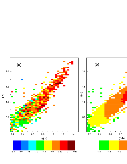
Figure 5: The mean [Fe/H] as a function of (d-n) and (d-h) for 2200 stellar spectroscopic metallicity (panel a) and photometric metallicity estimates (panel b). The color scheme shows the mean values in all 0.04 mag by 0.04 mag large pixels.

Figure 6: The residuals between the spectroscopic metallicity and photometric metallicity estimates based on equation (2) function as $d-n$. Stars within color range $d-h<$ 0.6 have rms scatter of 0.5 dex, while stars with $d-h>$ 0.6 have an rms scatter of 0.3 dex.

Figure 7: The metallicity distribution for 160 000 MS stars.

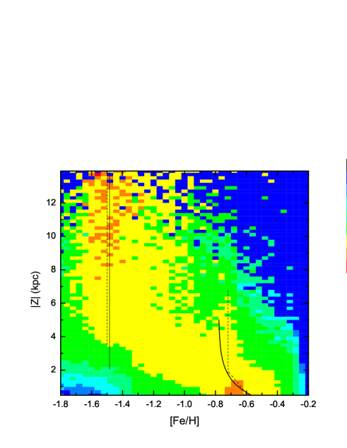
Figure 8: The resulting conditional metallicity probability distribution of 160 000 MS stars for a given Z and $p$([Fe/H]$|$Z). The color scheme shows the logarithm (base 10) of metallicity probability.

4 METALLICITY DISTRIBUTION

It is well known that the chemical abundance of stellar population contains much information about the Galaxy formation and evolution. The study of stellar metallicity distribution in the Galaxy has been an important subject of photometric and spectroscopic surveys (Perryman et al., 2001; Keller et al., 2007; Eisenstein et al., 2011). In this study, we want to explore possible stellar metallicity distribution as a function of position. The metallicity distribution for all MS stars as a function of vertical distance $|Z|$ is obtained in section 4.1. We first discuss several features which can be directly found. The detailed behaviors of metallicity distribution are described in the following sections.

4.1 The metallicity distribution as a function of vertical distance Z

According to the sample selected criteria in section 2.1, about 160 000 stars are extracted from 67 fields at median and high latitudes. Since stellar metallicity distribution at high Galactic latitudes are not strongly related to the radial distribution (Ivezić et al., 2008), they are well suited to study the vertical metallicity distribution of the Galaxy. The data selected cover a substantial range of $0.5<|Z|\leq 14~{}\rm{kpc}$. Figure 8 shows the resulting conditional metallicity probability distribution of 160 000 MS stars for a given Z and $p$([Fe/H]$|$Z). This distribution is computed as metallicity histograms in a narrow Z slices and normalized by the total number of stars in a given Z slice (Ivezić et al., 2008). The probability density derived at an interval of 0.2 kpc in Z distance and 0.04 dex in metallicity is shown on logarithmic scale.

From Figure 8, it is clear that there is a shift from metal-rich stars to metal-poor ones with the increasing of vertical distance. From Figure 8, in the interval $|Z|\leq 2~{}\rm{kpc}$, most stars with metallicity richer than $\rm{[Fe/H]}=-1$ belong to the thin disk stars and the stellar metallicity smoothly decreases with distance from the Galactic plane. Stars in interval $2<|Z|\leq 5~{}\rm{kpc}$ include both metal-poor and metal-rich stars, there is a mixture of the halo stars and the thick disk stars. It can be found that there is a unclear peak of the stellar metallicity distribution at $\rm{[Fe/H]}=-0.7$ (corresponding to the thick disk). This result is consistent with that result of Allende et al. (2006), who found the thick disc with a maximum at $\rm{[Fe/H]}=-0.7$. From Figure 8, we can see that most stars in interval $|Z|>5~{}\rm{kpc}$ are metal-poor stars, and the stellar metallicity distribution peaks at about $-1.5$ which is consistent with the previous work. Allende et al. (2006) found that the halo stars exhibit a broad range of metallicity, with a peak at $\rm{[Fe/H]}\simeq-1.4$. An (2013) considered that the metallicity distribution function of the Galactic halo can be adequately fit using a single Gaussian with a peak at $\rm{[Fe/H]}=-1.5$. The metallicity of the halo component appears to be spatially invariant, so there is little or no metallicity gradient in the halo.

From Figure 8, we can see that the stars in interval $2<|Z|\leq 5~{}\rm{kpc}$ include both metal-poor and metal-rich stars. Stars exhibit a broad range of metallicity. The metallicity distribution is mainly in range from $-1.7$ to $-0.5$, indicating that there is a mixture of the halo and the thick disk components. The metal-rich stars extend beyond 4–5 kpc from the plane and the stars are dominated by the halo stars in the interval $|Z|>5~{}\rm{kpc}$ advocating an edge of the Galactic thick disk at about 5 kpc above and below the plane. Based on our observation, we conclude that the possible cutoff of the thick disk stars is about 5 kpc above and below the Galactic plane. Majewski et al. (1992) considered the cutoff of the Galactic thick disk at about 5.5 kpc above the Galactic plane. Ivezić et al. (2008) analyzed SDSS DR6 photometric data and pointed out that it seems more likely that the disk is indeed traceable to beyond 5 kpc from the plane.

Ivezić et al. (2008) represented a model for $p$([Fe/H]$|$Z) of the Galaxy in the range of $0.5<|Z|\leqslant 10~{}\rm{kpc}$. The solid lines in Figure 8 show the mean metallicity of the disk and the halo for Ivezić et al. (2008). In their model, the mean halo metallicity distribution is spatially invariant ($\rm{[Fe/H]}=-1.46$) and the median metallicity for the disk component in the $0.5<|Z|\leqslant 5~{}\rm{kpc}$ range can be described as the curve in Figure 8. The dash lines in Figure 8 show the mean metallicity for the halo and the disk in our study. From Figure 8, we can find that the mean metallicity of the disk of our study is slightly richer than those of Ivezić et al. (2008) in the range of $2<|Z|\leqslant 5~{}\rm{kpc}$. However, the mean metallicity of the halo in our study is agree with the result of Ivezić et al. (2008).

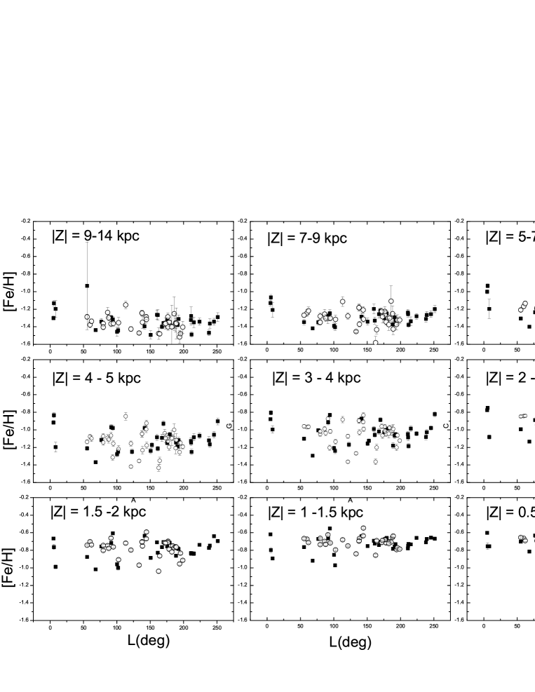
Figure 9: The mean metallicity distribution as a function of Galactic longitude in different distance intervals. Each panel corresponds to a narrow $|Z|$ range which labeled in each panel.

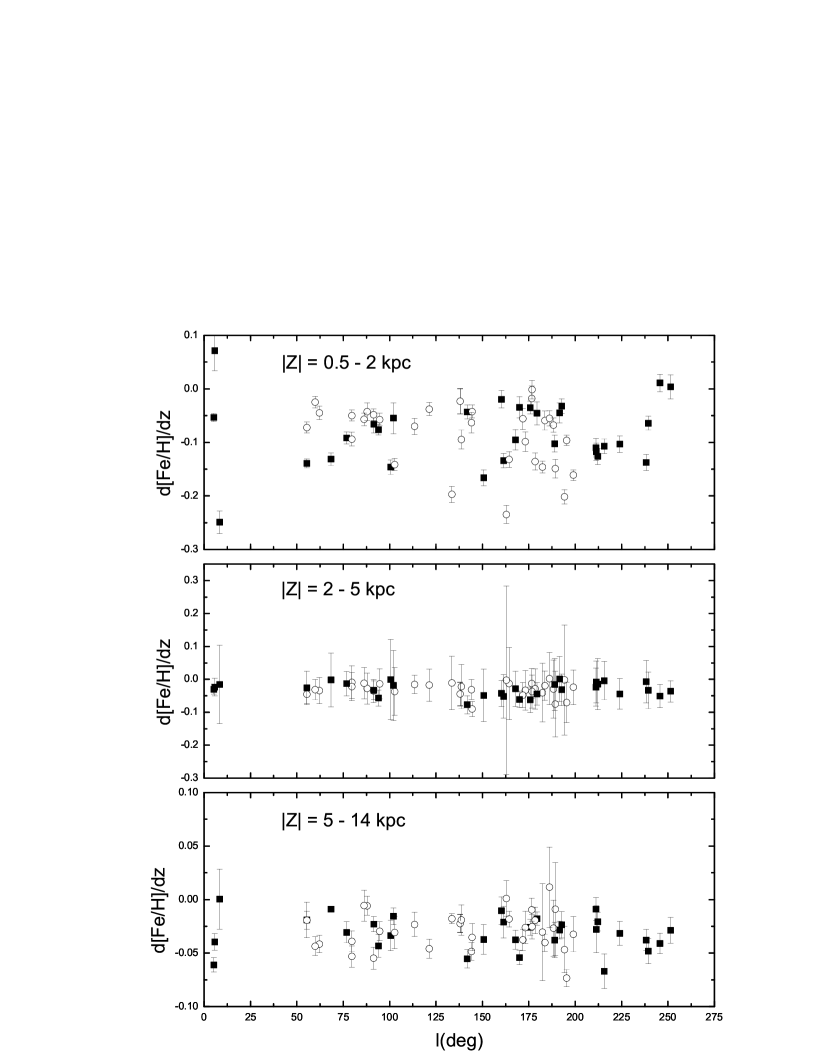
Figure 10: The metallicity gradient distribution as a function of Galactic longitude for the thin disk, the thick disk and the halo are shown.

4.2 Metallicity variation with Galactic longitude

Mean metallicity distribution of each BATC field as a function of Galactic longitude for different $|Z|$ distance intervals are presented in Figure 9. The panels from left to right and from top to bottom correspond to different distances from the Galactic plane, respectively. The mean metallicity shift from metal-rich to metal-poor with the increase of distance from the Galactic plane can be found in Figure 9. The solid points represent the south Galactic latitude fields, the open square points represent the north Galactic latitude fields. As shown in Figure 9, at any distance interval, the variation of the mean metallicity distributions with the Galactic longitude is almost flat. Ivezić et al. (2008) found that the metallicity distribution of the disk and the halo shifts toward higher metallicity in the region where affected by the Monoceros stream. Bilir et al. (2008) found the dependence of the Galactic model parameters on the Galactic longitude. However, no strong relation between the mean metallicity and Galactic longitude is found in our work.

The mean metallicity in interval $9<|Z|\leqslant 14~{}\rm{kpc}$ is around of $-1.34\pm 0.1\rm{dex}$. In interval $5<|Z|\leqslant 9~{}\rm{kpc}$, our result indicates that the mean metallicity is $\sim-1.25$. The mean metallicity decreases from $-0.90$ to $-1.13$ in intervals $2<|Z|\leqslant 5~{}\rm{kpc}$. The mean metallicity decreases from $-0.65$ to $-0.78$ in intervals $|Z|\leqslant 2~{}\rm{kpc}$. Ivezić et al. (2008) found that the median metallicity smoothly decreases with distance from the Galactic plane from $-$0.6 at 500 pc to $-$0.8 beyond several kpc. The work of Schlesinger et al. (2012) indicated that the metallicity distribution function of both G and K dwarf become more metal-poor with the increasing $|Z|$ from 0.2 to 2.3 kpc.

4.3 The vertical metallicity gradient

Detailed information about the vertical metallicity gradient can provide important clue about the formation scenario of stellar population. Here, we use the mean metallicity of each BATC field to derive the vertical metallicity gradient. The metallicity gradients for all the fields in three different $|Z|$ intervals, $|Z|\leq 2~{}\rm{kpc}$ (the thin disk), $2<|Z|\leqslant 5~{}\rm{kpc}$ (the thick disk) and $5<|Z|\leqslant 14~{}\rm{kpc}$ (the halo), are given in Figure 10. Compared with the typical error bars, there are no variations in the gradients with Galactic longitude for the three different components.

From Figure 10, we can find that the mean gradient of halo is about $-0.03\pm 0.02$ dex kpc^-1 ($5<|Z|\leqslant 14~{}\rm{kpc}$), which is essentially in agreement with the previous conclusions (Du et al., 2004; Ak et al., 2006; Yaz & Karaali, 2010; Peng et al., 2012). A metallicity gradient of the halo ($|Z|>5~{}\rm{kpc}$), $\rm{d[Fe/H]/dz}=-0.05$ dex kpc^-1, was found by Peng et al. (2012). Yaz & Karaali (2010) detected $\rm{d[Fe/H]/dz}=-0.01$ dex kpc^-1 for the inner spheroid. Ivezić et al. (2008) found that the halo metallicity distribution is remarkably uniform. No metallicity gradient found in the halo is consistent with the merger or accretion origin of the Galactic halo.

At distance $0.5<|Z|\leqslant 2~{}\rm{kpc}$, the mean vertical abundance gradient d[Fe/H]/dz is about $\sim-0.1\pm 0.02$ dex kpc^-1. This value is consistent with the result of Ivezić et al. (2008). They detected a vertical metallicity gradient for disk stars (0.1–0.2 dex kpc ^-1). However, our result is less than the results of previous works. Peng et al. (2012) found a metallicity gradient d[Fe/H]/dz $\sim-0.21\pm 0.05$ dex kpc^-1 in the range $|Z|\leq 2~{}\rm{kpc}$. The metallicity gradient was determined to be d[Fe/H]/dz $\sim-0.37$ dex kpc^-1 for $|Z|<4~{}\rm{kpc}$ in the work of Du et al. (2004). The range of our metallicity estimates only cover from $-0.2$ to $-1.8$. The cutoff of the extreme metal-rich disk stars may result in a little metallicity gradient in the thin disk.

Recently, the disk of Galaxy has been extensively studied (Bensby et al., 2003; Bilir et al., 2012), especially the thick disk. As shown in Figure 8, a significant mixture of the Galactic components can be found in the distance interval $2<|Z|\leqslant 5~{}\rm{kpc}$. For a long time, the metallicity distribution function of the thick disk was thought to be cut off below $\rm{[Fe/H]}=-1$. Recently, several surveys (Morrison, 1993; Beers et al., 1999; Katz et al., 1999; Beers et al., 2002) argued that the thick disk includes stars as metal-deficient as [Fe/H] $\sim-1.6$. However, the metal-weak thick disk appears to be minor constituent of the entire thick disk. Most metal-poor stars in the thick disk belong to the halo stars. Here, stars with [Fe/H] $>-1$ in the region $2<|Z|\leqslant 5~{}\rm{kpc}$ are selected to determine the metallicity gradient for the thick disk. There is a metallicity gradient $\sim-0.03\pm 0.02$ dex kpc^-1 in the thick disk which is consistent with the result of Allende et al. (2006). They found that no vertical metallicity gradient is apparent in this well-sampled region of the thick disk. The absence of metallicity gradient in the thick disk favors the conclusion that the thick disk was formed through the merger or accretion of the nearby dwarf galaxies.

5 SUMMARY AND CONCLUSION

Based on the stellar atmospheric parameters from SDSS spectra for $\sim 2200$ MS stars which were also observed by BATC photometric system, we develop the polynomial photometric calibration method to evaluate the stellar effective temperature and metallicity for BATC photometric data. This calibration method has been applied to about 160 000 MS stars from 67 BATC observed fields. The color index and magnitude selected criteria are used to choose the MS stars. The star sample in this paper, 160 000 MS stars, are much more than that in our previous work (Peng et al., 2012) which used 40 000 MS stars to derive the metallicity distribution of the Galaxy. The photometric effective temperature method is capable of deriving effective temperature with accuracy of 1.3 % and the photometric metallicity estimate with error about 0.5 dex.

According to the derived metallicities of all sample stars, we find that most stars in interval $|Z|>5~{}\rm{kpc}$ are metal-poor stars which correspond to the halo component. There is a peak of the stellar metallicity distribution at about $-1.5$ in this interval. The halo metallicity distribution seems invariant with the distance from the plane while the mean thin disk (0.5 $<|Z|\leq 2~{}\rm{kpc}$) metallicity smoothly decreases from $-0.65$ to $-0.78$ with distance from the Galactic plane. In interval $2<|Z|\leqslant 5~{}\rm{kpc}$, there is a mixture of the halo stars and the thick disk stars. The peak of the metallicity distribution for the thick disk is about $-0.7$. We believe that the possible cutoff of the thick disk stars is about 5 kpc above and below the Galactic plane. At any distance interval, the variation of the mean metallicity distributions with Galactic longitude is almost flat.

There is a mean vertical metallicity gradient d[Fe/H]/dz = $-0.1$ dex kpc^-1 for the thin disk stars ($0.5<|Z|\leqslant 2~{}\rm{kpc}$). Stars with [Fe/H] $>-1$ and $2<|Z|\leqslant 5~{}\rm{kpc}$ are selected to determine the metallicity gradient for the thick disk. There is a vertical metallicity gradient $\sim-0.03\pm 0.02$ dex kpc^-1 in the thick disk. Meanwhile, the mean vertical gradient of the halo is about $-0.03\pm 0.02$ dex kpc^-1 ($5<|Z|\leqslant 14~{}\rm{kpc}$). The absence of the vertical gradient in the thick disk and the halo favor the conclusion that the thick disk and the halo may be formed through merger or acceration. The variations of the vertical gradient for different Galaxy components with Galactic longitude are flat.

References

- Ak et al. (2006) Ak S., Bilir S., Karaali S., Buser R., 2007, AN, 328, 169
- Allende et al. (2006) Allende Prieto C., Beers T. C., Wilhelm R., Newberg H. J., Rockosi C. M., Yanny B., Lee Y. S., 2006, ApJ, 636, 804
- Allende et al. (2008) Allende Prieto C. et al., 2008, AJ, 136, 2070
- An (2013) An D. et al., 2013, ApJ, 763, 65
- Bahcall & Soneira (1980) Bahcall J. N., Soneira R. M., 1980, ApJ, 238, 17
- Beers et al. (1999) Beers T. C., Rossi S., Norris J. E., Ryan S. G., Shefler T., 1999, AJ, 117, 981
- Beers et al. (2002) Beers T. C. et al., 2002, AJ, 124, 931
- Beers & Christlieb (2005) Beers T. C., Christlieb N., 2005, ARAA, 43, 531
- Belokurov et al. (2006) Belokurov V. et al., 2006, ApJ, 642, 137
- Bensby et al. (2003) Bensby T., Feltzing S., Lundstrom I., 2003, A&A, 410, 527
- Bilir et al. (2008) Bilir S., Cabrera-Lavers A., Karaali S., Ak S., Yaz E., Lpez-Corredoira M., 2008, PASA, 25, 69
- Bilir et al. (2012) Bilir S. et al., 2012, MNRAS, 421, 3362
- Bovy et al. (2012) Bovy J., Rix H.- W., Liu C., Hogg D. W., Beers T. C., Lee Y. S., 2012, ApJ, 753, 148
- Casagrande et al. (2006) Casagrande L., Portinari L., Flynn C., 2006, MNRAS, 373, 13
- Chen et al. (2011) Chen Y. Q., Zhao G., Carrell K., Zhao J. K., 2011, AJ, 142, 184
- de Jong et al. (2010) de Jong J. T. A., Yanny B., Rix H.-W., Dolphin A. E., Martin N. F., Beers T. C., 2010, ApJ, 714, 663
- Du et al. (2003) Du C. H. et al., 2003, A&A , 407, 541
- Du et al. (2004) Du C. H. et al., 2004, AJ, 128, 2265
- Du et al. (2006) Du C. H. et al., 2006, MNRAS, 372, 1304
- Duffau et al. (2006) Duffau S., Zinn R., Vivas A. K., Carraro G., Méndez R.A., Winnick R., Gallart C., 2006, ApJ. Lett., 636, 97
- Eggen et al. (1962) Eggen O. J., Lynden-Bell D., Sandage A. R., 1962, ApJ, 136, 748
- Eisenstein et al. (2011) Eisenstein D. J. et al., 2011, AJ, 142, 72
- Fan et al. (1996) Fan X. H. et al., 1996, AJ, 112, 628
- Gilmore & Reid (1983) Gilmore G., Reid N., 1983, MNRAS, 202, 1025
- Gilmore et al. (1989) Gilmore G., Wyse R. F. G., Kuijken K., 1989, ARA&A, 27, 555
- Gunn et al. (1998) Gunn J. E. et al., 1998, AJ, 116, 3040
- Ivezić et al. (2000) Ivezić Ž. et al., 2000, AJ, 120, 963
- Ivezić et al. (2008) Ivezić Ž. et al., 2008, ApJ, 684, 287
- Ivezić et al. (2012) Ivezić Ž., Beers T. C., Jurić M., 2012, ARAA, 50, 251
- Jurić et al. (2008) Jurić M. et al., 2008, ApJ, 673, 864
- Karaali et al. (2003a) Karaali S., AK S. G., Bilir S., Karatas Y., Gilmore G., 2003a, MNRAS, 343, 1013
- Karaali et al. (2003b) Karaali S., Bilir S., Karatas Y., Ak S. G., 2003b, PASA, 20, 165
- Karatas et al. (2009) Karatas Y., Kilic M., Günes O., Limboz F., 2009, PASP, 26, 1
- Katz et al. (1999) Katz D. et al., 1999, Ap&SS, 265, 221
- Keller et al. (2007) Keller S. C. et al., 2007, PASA, 24, 1
- Kroupa et al. (1993) Kroupa P., Tout C. A., Gilmore G., 1993, MNRAS, 262, 545
- Lang (1992) Lang K. R. 1992, Astrophysical Data I, Planets and Stars. Springer-Verlag, Berlin
- Lee et al. (2008a) Lee Y. S. et al., 2008a, AJ, 136, 2022
- Lee et al. (2008b) Lee Y. S. et al., 2008b, AJ, 136, 2050
- Majewski et al. (1992) Majewski S. R. 1992, ApJS, 78, 87
- Majewski et al. (1996) Majewski S. R., Munn J. A., Hawley S. L., 1996, ApJ, 459, 73
- Majewski et al. (2003) Majewski S. R., Skrutskie M. F., Weinberg M. D., Ostheimer J. C., 2003, ApJ, 599, 1082
- Morrison (1993) Morrison H. L. 1993, AJ, 105, 539
- Newberg et al. (2002) Newberg H. J. et al., 2002, ApJ, 569, 245
- Nordström et al. (2004) Nordström B. et al., 2004, A&A, 418, 989
- Norris & Ryan (1991) Norris J. E., Ryan S. G., 1991, ApJ, 380, 403
- Ojha et al. (1996) Ojha D. K., Bienayme O., Robin A. C., Creze M., Mohan V., 1996, A&A, 311, 456
- Oke & Gunn (1983) Oke J. B., Gunn J. E., 1983, ApJ, 266, 713
- Peng et al. (2012) Peng X. Y., Du C. H., Wu Z. Y., 2012, MNRAS, 422, 2756
- Perryman et al. (2001) Perryman M. A. C. et al., 2001, A&A, 369, 339
- Prior et al. (2009) Prior S. L., Da Costa G. S., Keller S. C., Murphy, S. J., 2009, ApJ, 691,306
- Rocha-Pintoet al. (2003) Rocha-Pinto H. J., Majewski S. R., Skrutskie M. F., Crane J. D., 2003, ApJ, 594, 115
- Sandage (1969) Sandage A. 1969, ApJ, 158, 1115
- Smee et al. (2012) Smee S. et al., 2012, preprint (arXiv:1208.2233)
- Schwarzschild et al. (1955) Schwarzschild M., Searle L., Howard R., 1955, ApJ, 122, 353
- Schlegel et al. (1998) Schlegel D. J., Finkbeiner D. P., Davis M., 1998, ApJ, 500, 525
- Schlesinger et al. (2012) Schlesinger K. J. et al., 2012, ApJ, 761, 160
- Searle & Zinn (1978) Searle L., Zinn R., 1978, ApJ, 225, 357
- Siegel et al. (2009) Siegel M. H., Karatas Y., Reid I. N., 2009, MNRAS, 395, 1569
- Vivas et al. (2001) Vivas A. K. et al., 2001, ApJ, 554, 33
- Yanny et al. (2000) Yanny B. et al., 2000, ApJ, 540, 825
- Yaz & Karaali (2010) Yaz E., Karaali S., 2010, NewA, 15, 234
- York et al. (2000) York D. G. et al., 2000, AJ, 120, 1579
- Zhou et al. (2003) Zhou X. et al., 2003, AA, 397, 361