Slot Games for Detecting Timing Leaks of Programs

Abstract

In this paper we describe a method for verifying secure information flow of programs, where apart from direct and indirect flows a secret information can be leaked through covert timing channels. That is, no two computations of a program that differ only on high-security inputs can be distinguished by low-security outputs and timing differences. We attack this problem by using slot-game semantics for a quantitative analysis of programs. We show how slot-games model can be used for performing a precise security analysis of programs, that takes into account both extensional and intensional properties of programs. The practicality of this approach for automated verification is also shown.

1 Introduction

Secure information flow analysis is a technique which performs a static analysis of a program with the goal of proving that it will not leak any sensitive (secret) information improperly. If the program passes the test, then we say that it is secure and can be run safely. There are several ways in which secret information can be leaked to an external observer. The most common are direct and indirect leakages, which are described by the so-called non-interference property [13, 18]. We say that a program satisfies the non-interference property if its high-security (secret) inputs do not affect its low-security (public) outputs, which can be seen by external observers.

However, a program can also leak information through its timing behaviour, where an external observer can measure its total running time. Such timing leaks are difficult to detect and prevent, because they can exploit low-level implementation details. To detect timing leaks, we need to ensure that the total running time of a program do not depend on its high-security inputs.

In this paper we describe a game semantics based approach for performing a precise security analysis. We have already shown in [8] how game semantics can be applied for verifying the non-interference property. Now we use slot-game semantics to check for timing leaks of closed and open programs. We focus here only on detecting covert timing channels, since the non-interference property can be verified similarly as in [8]. Slot-game semantics was developed in [11] for a quantitative analysis of Algol-like programs. It is suitable for verifying the above security properties, since it takes into account both extensional (what the program computes) and intensional (how the program computes) properties of programs. It represents a kind of denotational semantics induced by the theory of operational improvement of Sands [19]. Improvement is a refinement of the standard theory of operational approximation, where we say that one program is an improvement of another if its execution is more efficient in any program context. We will measure efficiency of a program as the sum of costs associated with basic operations it can perform. It has been shown that slot-game semantics is fully abstract (sound and complete) with respect to operational improvement, so we can use it as a denotational theory of improvement to analyse programming languages.

The advantages of game semantics (denotational) based approach for verifying security are several. We can reason about open programs, i.e. programs with non-locally defined identifiers. Moreover, game semantics is compositional, which enables analysis about program fragments to be combined into an analysis of a larger program. Also the model hides the details of local-state manipulation of a program, which results in small models with maximum level of abstraction where are represented only visible input-output behaviours enriched with costs that measure their efficiency. All other behaviour is abstracted away, which makes this model very suitable for security analysis. Finally, the game model for some language fragments admits finitary representation by using regular languages or CSP processes [10, 6], and has already been applied to automatic program verification. Here we present another application of algorithmic game semantics for automatically verifying security properties of programs.

Related work.

The most common approach to ensure security properties of programs is by using security-type systems [14]. Here for every program component are defined security types, which contain information about their types and security levels. Programs that are well-typed under these type systems satisfy certain security properties. Type systems for enforcing non-interference of programs have been proposed by Volpano and Smith in [20], and subsequently they have been extended to detect also covert timing channels in [21, 2]. A drawback of this approach is its imprecision, since many secure programs are not typable and so are rejected. A more precise analysis of programs can be achieved by using semantics-based approaches [15].

2 Syntax and Operational Semantics

We will define a secure information flow analysis for Idealized Algol (IA), a small Algol-like language introduced by Reynolds [16] which has been used as a metalanguage in the denotational semantics community. It is a call-by-name $\mathop{\mathstrut{\lambda}}\nolimits$-calculus extended with imperative features and locally-scoped variables. In order to be able to perform an automata-theoretic analysis of the language, we consider here its second-order recursion-free fragment (IA₂ for short). It contains finitary data types $D$: $\mathsf{int}_{n}=\{0,\ldots,n-1\}$ and $\mathsf{bool}=\{tt,ff\}$, and first-order function types: $T::=B\mid B\rightarrow T$, where $B$ ranges over base types: expressions ($\mathsf{exp}D$), commands ($\mathsf{com}$), and variables ($\mathsf{var}D$).

Syntax of the language is given by the following grammar:

$$\begin{array}[]{l}M::=\!\!x\!\mid\!v\!\mid\!\mathsf{skip}\mid\!\mathsf{diverge}\mid M\,\mathsf{op}\,M\mid M\mathchar 24635\relax\;\!\!M\mid\mathsf{if}\,M\,\mathsf{then}\,M\,\mathsf{else}\,M\!\mid\!\mathsf{while}\,M\,\mathsf{do}\,M\\ \ \qquad\mid M:=M\mid!M\mid\mathsf{new}_{D}\>x\!:=\!v\>\mathsf{in}\>M\mid\mathsf{mkvar}_{D}MM\mid\!\mathop{\mathstrut{\lambda}}\nolimits x.M\mid MM\end{array}$$

where $v$ ranges over constants of type $D$.

Typing judgements are of the form $\Gamma\vdash M:T$, where $\Gamma$ is a type context consisting of a finite number of typed free identifiers. Typing rules of the language are standard [1], but the general application rule is broken up into the linear application and the contraction rule .

  $\Gamma\vdash M:B\to T$         $\Delta\vdash N:B$               $\Gamma,\Delta\vdash MN:T$           $\Gamma,x_{1}:T,x_{2}:T\vdash M:T^{\prime}$     $\Gamma,x:T\vdash M[x/x_{1},x/x_{2}]:T^{\prime}$

We use these two rules to have control over multiple occurrences of free identifiers in terms during typing.

Any input/output operation in a term is done through global variables, i.e. free identifiers of type $\mathsf{var}D$. So an input is read by de-referencing a global variable, while an output is written by an assignment to a global variable.

The operational semantics is defined in terms of a small-step evaluation relation using a notion of an evaluation context [9]. A small-step evaluation (reduction) relation is of the form:

$$\Gamma\vdash M,\mathrm{s}\longrightarrow M^{\prime},\mathrm{s}^{\prime}$$

where $\Gamma$ is a so-called $\mathsf{var}$-context which contains only identifiers of type $\mathsf{var}D$; $\mathrm{s}$, $\mathrm{s}^{\prime}$ are $\Gamma$-states which assign data values to the variables in $\Gamma$; and $M$, $M^{\prime}$ are terms. The set of all $\Gamma$-states will be denoted by $St(\Gamma)$.

Evaluation contexts are contexts containing a single hole which is used to identify the next sub-term to be evaluated (reduced). They are defined inductively by the following grammar:

$$\begin{array}[]{l}E::=[-]\mid EM\mid E\mathchar 24635\relax\;\!M\mid\mathsf{skip}\mathchar 24635\relax\;\!E\mid E\,\mathsf{op}\,M\mid v\,\mathsf{op}\,E\mid\mathsf{if}\,E\,\mathsf{then}\,M\,\mathsf{else}\,M\mid M:=E\mid E:=v\mid!E\end{array}$$

The operational semantics is defined in two stages. First, a set of basic reduction rules are defined in Table 1. We assign different (non-negative) costs to each reduction rule, in order to denote how much computational time is needed for a reduction to complete. They are only descriptions of time and we can give them different interpretations describing how much real time they denote. Such an interpretation can be arbitrarily complex. So the semantics is parameterized on the interpretation of costs. Notice that we write $\mathrm{s}\otimes(x\mapsto v)$ to denote a $\{\Gamma,x\}$-state which properly extends $\mathrm{s}$ by mapping $x$ to the value $v$.

$\begin{array}[]{@{}l}\Gamma\vdash n_{1}\,\mathsf{op}\,n_{2},\mathrm{s}\longrightarrow^{k_{op}}n,\mathrm{s},\ \textrm{where}\,n=n_{1}\mathrm{op}n_{2}\\ \Gamma\vdash\mathsf{skip}\mathchar 24635\relax\;\mathsf{skip},\mathrm{s}\longrightarrow^{k_{seq}}\mathsf{skip},\mathrm{s}^{\prime}\\ \Gamma\vdash\mathsf{if}\,tt\,\mathsf{then}\,M_{1}\,\mathsf{else}M_{2},\mathrm{s}\longrightarrow^{k_{if}}M_{1},\mathrm{s}\\ \Gamma\vdash\mathsf{if}\,ff\,\mathsf{then}\,M_{1}\,\mathsf{else}M_{2},\mathrm{s}\longrightarrow^{k_{if}}M_{2},\mathrm{s}\\ \Gamma\vdash x\,\raisebox{0.27986pt}{:}{=}\,v^{\prime},\mathrm{s}\otimes(x\mapsto v)\longrightarrow^{k_{asg}}\mathsf{skip},\mathrm{s}\otimes(x\mapsto v^{\prime})\\ \Gamma\vdash!x,\mathrm{s}\otimes(x\mapsto v)\longrightarrow^{k_{der}}v,\mathrm{s}\otimes(x\mapsto v)\\ \Gamma\vdash(\mathop{\mathstrut{\lambda}}\nolimits x.M)M^{\prime},\mathrm{s}\longrightarrow^{k_{app}}M[M^{\prime}/x],\mathrm{s}\\ \Gamma\vdash\mathsf{new}_{D}\,x\,\raisebox{0.27986pt}{:}{=}\,v\,\mathsf{in}\,\mathsf{skip},\mathrm{s}\longrightarrow^{k_{new}}\mathsf{skip},\mathrm{s}\end{array}$

Table 1: Basic Reduction Rules

We also have reduction rules for iteration, local variables, and $\mathsf{mkvar}_{D}$ construct, which do not incur additional costs.

$\Gamma\vdash\mathsf{while}\,b\,\mathsf{do}\,M,\mathrm{s}\longrightarrow\mathsf{if}\,b\,\mathsf{then}\,(M\mathchar 24635\relax\;\mathsf{while}\,b\,\mathsf{do}\,M)\,\mathsf{else\,skip},\mathrm{s}$

        $\Gamma,y\vdash M[y/x],\mathrm{s}\otimes(y\mapsto v)\longrightarrow M^{\prime},\mathrm{s^{\prime}}\otimes(y\mapsto v^{\prime})$     $\Gamma\vdash\mathsf{new}_{D}\,x\,\raisebox{0.27986pt}{:}{=}\,v\,\mathsf{in}\,M,\mathrm{s}\longrightarrow\mathsf{new}_{D}\,x\,\raisebox{0.27986pt}{:}{=}\,v^{\prime}\,\mathsf{in}\,M^{\prime}[x/y],\mathrm{s^{\prime}}$

$\Gamma\vdash(\mathsf{mkvar}_{D}\,M_{1}M_{2})\,\raisebox{0.27986pt}{:}{=}\,v,\mathrm{s}\longrightarrow M_{1}v,\mathrm{s}\qquad\Gamma\vdash!(\mathsf{mkvar}_{D}\,M_{1}M_{2}),\mathrm{s}\longrightarrow M_{2},\mathrm{s}$

Next, the in-context reduction rules for arbitrary terms are defined as:

       $\Gamma\vdash M,\mathrm{s}\longrightarrow^{n}M^{\prime},\mathrm{s^{\prime}}$     $\Gamma\vdash E[M],\mathrm{s}\longrightarrow^{n}E[M^{\prime}],\mathrm{s^{\prime}}$

The small-step evaluation relation is deterministic, since arbitrary term can be uniquely partitioned into an evaluation context and a sub-term, which is next to be reduced.

We define the reflexive and transitive closure of the small-step reduction relation as follows:

  $\Gamma\vdash M,\mathrm{s}\longrightarrow^{n}M^{\prime},\mathrm{s^{\prime}}$      $\Gamma\vdash M,\mathrm{s}{}^{n}M^{\prime},\mathrm{s^{\prime}}$      $\Gamma\vdash M,\mathrm{s}{}^{n}M^{\prime},\mathrm{s^{\prime}}$         $\Gamma\vdash M^{\prime},\mathrm{s^{\prime}}{}^{n^{\prime}}M^{\prime\prime},\mathrm{s^{\prime\prime}}$                 $\Gamma\vdash M,\mathrm{s}{}^{n+n^{\prime}}M^{\prime\prime},\mathrm{s^{\prime\prime}}$

Now a theory of operational improvement is defined [19]. Let $\Gamma\vdash M:\mathsf{com}$ be a term, where $\Gamma$ is a $\mathsf{var}$-context. We say that $M$ terminates in $n$ steps at state $\mathrm{s}$, written $M,\mathrm{s}\Downarrow^{n}$, if $\Gamma\vdash M,\mathrm{s}{}^{n}\mathsf{skip},\mathrm{s}^{\prime}$ for some state $\mathrm{s}^{\prime}$. If $M$ is a closed term and $M,\emptyset\Downarrow^{n}$, then we write $M\Downarrow^{n}$. If $M\Downarrow^{n}$ and $n\leq n^{\prime}$, we write $M\Downarrow^{\leq n^{\prime}}$. We say that a term $\Gamma\vdash M:T$ may be improved by $\Gamma\vdash N:T$, denoted by $\Gamma\vdash M\gtrsim N$, if and only if for all contexts $C[-]$, if $C[M]\Downarrow^{n}$ then $C[N]\Downarrow^{\leq n}$. If two terms improve each other they are considered improvment-equivalent, denoted by $\Gamma\vdash M\thickapprox N$.

Let $\Gamma,\Delta\vdash M:T$ be a term where $\Gamma$ is a $var$-context and $\Delta$ is an arbitrary context. Such terms are called split terms, and we denote them as $\Gamma|\Delta\vdash M:T$. If $\Delta$ is empty, then these terms are called semi-closed. The semi-closed terms have only some global variables, and the operational semantics is defined only for them. We say that a semi-closed term $h:\mathsf{varD}|-\vdash M:\mathsf{com}$ does not have timing leaks if the initial value of the high-security variable $h$ does not influence the number of reduction steps of $M$. More formally, we have:

Definition 1.

A semi-closed term $h:\mathsf{varD}|-\vdash M:\mathsf{com}$ has no timing leaks if

$$\begin{array}[]{ll}\mathop{\mathstrut{\forall}}\nolimits s_{1},s_{2}\in St(\{h\}).&s_{1}(h)\neq s_{2}(h)\mathrel{\wedge}\\ &h:\mathsf{varD}\vdash M,\mathrm{s_{1}}{}^{n_{1}}\mathsf{skip},\mathrm{s_{1}}^{\prime}\mathrel{\wedge}h:\mathsf{varD}\vdash M,\mathrm{s_{2}}{}^{n_{2}}\mathsf{skip},\mathrm{s_{2}}^{\prime}\\ &\Rightarrow n_{1}=n_{2}\end{array}$$ (1)

Definition 2.

We say that a split term $h:\mathsf{varD}|\Delta\vdash M:\mathsf{com}$ does not have timing leaks, where $\Delta=x_{1}:T_{1},\ldots,x_{k}:T_{k}$, if for all closed terms $\vdash N_{1}:T_{1},\ldots,\vdash N_{k}:T_{k}$, we have that the term $h:\mathsf{varD}|-\vdash M[N_{1}/x_{1},\ldots,N_{k}/x_{k}]:\mathsf{com}$ does not have timing leaks.

The formula (1) can be replaced by an equivalent formula, where instead of two evaluations of the same term we can consider only one evaluation of the sequential composition of the given term with another its copy [3]. So sequential composition enables us to place these two evaluations one after the other. Let $h:\mathsf{varD}\vdash M:\mathsf{com}$ be a term, we define $M^{\prime}$ to be $\alpha$-equivalent to $M[h^{\prime}/h]$ where all bound variables are suitable renamed. The following can be shown: $h\vdash M,\mathrm{s_{1}}{}^{n}\mathsf{skip},\mathrm{s_{1}}^{\prime}\mathrel{\wedge}h^{\prime}\vdash M^{\prime},\mathrm{s_{2}}{}^{n^{\prime}}\mathsf{skip},\mathrm{s_{2}}^{\prime}$ iff $h,h^{\prime}\vdash M\mathchar 24635\relax\;M^{\prime},\mathrm{s_{1}}\otimes\mathrm{s_{2}}{}^{n+n^{\prime}}\mathsf{skip\mathchar 24635\relax\;skip},\mathrm{s_{1}}^{\prime}\otimes\mathrm{s_{2}}^{\prime}$. In this way, we provide an alternative definition to formula (1) as follows. We say that a semi-closed term $h|-\vdash M:T$ has no timing leaks if

$$\begin{array}[]{ll}\mathop{\mathstrut{\forall}}\nolimits s_{1}\in St(\{h\}),s_{2}\in St(\{h^{\prime}\}).&\ s_{1}(h)\neq s_{2}(h^{\prime})\mathrel{\wedge}\\ &h,h^{\prime}\vdash M\mathchar 24635\relax\;M^{\prime},\mathrm{s_{1}}\otimes\mathrm{s_{2}}{}^{n_{1}}\mathsf{skip}\mathchar 24635\relax\;M^{\prime},\mathrm{s_{1}}^{\prime}\otimes\mathrm{s_{2}}{}^{n_{2}}\mathsf{skip\mathchar 24635\relax\;skip},\mathrm{s_{1}}^{\prime}\otimes\mathrm{s_{2}}^{\prime}\\ &\Rightarrow n_{1}=n_{2}\end{array}$$ (2)

3 Algorithmic Slot-Game Semantics

We now show how slot-game semantics for IA₂ can be represented algorithmically by regular-languages. In this approach, types are interpreted as games, which have two participants: the Player representing the term, and the Opponent representing its context. A game (arena) is defined by means of a set of moves, each being either a question move or an answer move. Each move represents an observable action that a term of a given type can perform. Apart from moves, another kind of action, called token (slot), is used to take account of quantitative aspects of terms. It represents a payment that a participant needs to pay in order to use a resource such as time. A computation is interpreted as a play-with-costs, which is given as a sequence of moves and token-actions played by two participants in turns. We will work here with complete plays-with-costs which represent the observable effects along with incurred costs of a completed computation. Then a term is modelled by a strategy-with-costs, which is a set of complete plays-with-costs. In the regular-language representation of game semantics [10], types (arenas) are expressed as alphabets of moves, computations (plays-with-costs) as words, and terms (strategies-with-costs) as regular-languages over alphabets.

Each type $T$ is interpreted by an alphabet of moves $\mathcal{A}_{[\![T]\!]}$, which can be partitioned into two subsets of questions $Q_{[\![T]\!]}$ and answers $A_{[\![T]\!]}$. For expressions, we have: $Q_{[\![\mathsf{exp}D]\!]}=\{\textit{q}\}$ and $A_{[\![\mathsf{exp}D]\!]}=D$, i.e. there are a question move q to ask for the value of the expression and values from $D$ are possible answers. For commands, we have: $Q_{[\![\mathsf{com}]\!]}=\{\textit{run}\}$ and $A_{[\![\mathsf{com}]\!]}=\{\textit{done}\}$, i.e. there are a question move run to initiate a command and an answer move done to signal successful termination of a command. For variables, we have: $Q_{[\![\mathsf{var}D]\!]}=\{\textit{read},\textit{write}(a)\,\mid\,a\in D\}$ and $A_{[\![\mathsf{var}D]\!]}=D\cup\{\textit{ok}\}$, i.e. there are moves for writing to the variable, $\textit{write}(a)$, acknowledged by the move ok, and for reading from the variable, we have a question move read, and an answer to it can be any value from $D$. For function types, we have $\mathcal{A}_{[\![B_{1}^{1}\to\ldots\to B_{k}^{k}\to B]\!]}=\sum_{1\leq i\leq k}\mathcal{A}_{[\![B_{i}]\!]}^{i}+\mathcal{A}_{[\![B]\!]}$, where $+$ means a disjoint union of alphabets. We will use superscript tags to keep record from which type of the disjoint union each move comes from. We denote the token-action by \raisebox{-.9pt} {\$}⃝. A sequence of $n$ token-actions \raisebox{-.9pt} {\$}⃝ will be written as \raisebox{-.9pt} {n}⃝.

For any ($\beta$-normal) term we define a regular language specified by an extended regular expression $R$. Apart from the standard operations for generating regular expressions, we will use some more specific operations. We define composition of regular expressions $R$ defined over alphabet $\mathcal{A}^{1}+\mathcal{B}^{2}+\{\raisebox{0.5pt}{\raisebox{-.9pt} {\$}⃝}\}$ and $S$ over $\mathcal{B}^{2}+\mathcal{C}^{3}+\{\raisebox{0.5pt}{\raisebox{-.9pt} {\$}⃝}\}$ as follows:

$$\begin{array}[]{l}R\mathbin{\raise 2.58334pt\hbox{\small\oalign{\hfil$\scriptscriptstyle\mathrm{o}$\hfil\cr\hfil$\scriptscriptstyle\mathrm{9}$\hfil}}}_{\mathcal{B}^{2}}S=\{w\big{[}s/a^{2}\cdot b^{2}\big{]}\ \mid\ w\in S,a^{2}\cdot s\cdot b^{2}\in R\}\end{array}$$

where $R$ is a set of words of the form $a^{2}\cdot s\cdot b^{2}$, such that $a^{2}$, $b^{2}\in\mathcal{B}^{2}$ and $s$ contains only letters from $\mathcal{A}^{1}$ and $\{\raisebox{0.5pt}{\raisebox{-.9pt} {\$}⃝}\}$. Notice that the composition is defined over $\mathcal{A}^{1}+\mathcal{C}^{3}+\{\raisebox{0.5pt}{\raisebox{-.9pt} {\$}⃝}\}$, and all letters of $\mathcal{B}^{2}$ are hidden. The shuffle operation $R\bowtie S$ generates the set of all possible interleavings from words of $R$ and $S$, and the restriction operation $R\mid_{\mathcal{A}^{\prime}}$ ($R$ defined over $\mathcal{A}$ and $\mathcal{A}^{\prime}\subseteq\mathcal{A}$) removes from words of $R$ all letters from $\mathcal{A}^{\prime}$.

If $w$, $w^{\prime}$ are words, $m$ is a move, and $R$ is a regular expression, define $m\cdot w\smallfrown w^{\prime}=m\cdot w^{\prime}\cdot w$, and $R\smallfrown w^{\prime}=\{w\smallfrown w^{\prime}\mid w\in R\}$. Given a word with costs $w$ defined over $\mathcal{A}+\{\raisebox{0.5pt}{\raisebox{-.9pt} {\$}⃝}\}$, we define the underlying word of $w$ as $w^{{\dagger}}=w\mid_{\{\raisebox{0.5pt}{\raisebox{-.9pt} {\$}⃝}\}}$, and the cost of $w$ as $w\mid_{\mathcal{A}}=\raisebox{0.5pt}{\raisebox{-.9pt} {n}⃝}$, which we denote as $|w|=n$.

The regular expression for $\Gamma\vdash M:T$ is denoted $[\![\Gamma\vdash M:T]\!]$ and is defined over the alphabet $\mathcal{A}_{[\![\Gamma\vdash T]\!]}=\big{(}\sum_{x:T^{\prime}\in\Gamma}\mathcal{A}_{[\![T^{\prime}]\!]}^{x}\big{)}+\mathcal{A}_{[\![T]\!]}+\{\raisebox{0.5pt}{\raisebox{-.9pt} {\$}⃝}\}$. Every word in $[\![\Gamma\vdash M:T]\!]$ corresponds to a complete play-with-costs in the strategy-with-costs for $\Gamma\vdash M:T$.

Free identifiers $x\in\Gamma$ are interpreted by the copy-cat regular expressions, which contain all possible computations that terms of that type can have. Thus they provide the most general closure of an open term.

$$\begin{array}[]{@{}l}[\![\Gamma,x:B_{1}^{x,1}\to\ldots B_{k}^{x,k}\to B^{x}\vdash x:B_{1}^{1}\to\ldots B_{k}^{k}\to B]\!]=\\ \qquad\qquad\qquad\qquad\displaystyle{\sum_{q\in Q_{[\![B]\!]}}}q\cdot q^{x}\cdot\big{(}\displaystyle{\sum_{1\leq i\leq k}}(\sum_{q_{1}\in Q_{[\![B_{i}]\!]}}q_{1}^{x,i}\cdot q_{1}^{i}\cdot\sum_{a_{1}\in A_{[\![B_{i}]\!]}}a_{1}^{i}\cdot a_{1}^{x,i})\big{)}^{*}\cdot\sum_{a\in A_{[\![B]\!]}}a^{x}\cdot a\end{array}$$

When a first-order non-local function is called, it may evaluate any of its arguments, zero or more times, and then it can return any value from its result type as an answer. For example, the term $[\![\Gamma,x:\mathsf{exp}D^{x}\vdash x:\mathsf{exp}D]\!]$ is modelled by the regular expression: $\textit{q}\cdot\textit{q}^{x}\cdot\sum_{n\in D}n^{x}\cdot n$.

The linear application is defined as:

$$[\![\Gamma,\Delta\vdash M\,N:T]\!]=[\![\Delta\vdash N:B^{1}]\!]\mathbin{\raise 2.58334pt\hbox{\small\oalign{\hfil$\scriptscriptstyle\mathrm{o}$\hfil\cr\hfil$\scriptscriptstyle\mathrm{9}$\hfil}}}_{\mathcal{A}_{[\![B]\!]}^{1}}[\![\Gamma\vdash M:B^{1}\to T]\!]$$

Since we work with terms in $\beta$-normal form, function application can occur only when the function term is a free identifier. In this case, the interpretation is the same as above except that we add the cost $k_{app}$ corresponding to function application. Notice that $k_{app}$ denotes certain number of \raisebox{-.9pt} {\$}⃝ units that are needed for a function application to take place. The contraction $[\![\Gamma,x:T^{x}\vdash M[x/x_{1},x/x_{2}]:T^{\prime}]\!]$ is obtained from $[\![\Gamma,x_{1}:T^{x_{1}},x_{2}:T^{x_{2}}\vdash M:T^{\prime}]\!]$, such that the moves associated with $x_{1}$ and $x_{2}$ are de-tagged so that they represent actions associated with $x$.

To represent local variables, we first need to define a (storage) ‘cell’ regular expression $\mathsf{cell}_{v}$ which imposes the good variable behaviour on the local variable. So $\mathsf{cell}_{v}$ responds to each $\textit{write}(n)$ with ok, and plays the most recently written value in response to read, or if no value has been written yet then answers the read with the initial value $v$. Then we have:

$$\begin{array}[]{l}\mathsf{cell}_{v}=(\textit{read}\cdot v)^{*}\cdot\big{(}\displaystyle{\sum_{n\in D}}\textit{write}(n)\cdot\textit{ok}\cdot(\textit{read}\cdot n)^{*}\big{)}^{*}\\ [\![\Gamma,x:\mathsf{var}D\vdash M]\!]\circ\mathsf{cell}_{v}^{x}=\big{(}[\![\Gamma,x:\mathsf{var}D\vdash M]\!]\cap(\mathsf{cell}_{v}^{x}\bowtie(\mathcal{A}_{[\![\Gamma\vdash B]\!]}+\raisebox{0.5pt}{\raisebox{-.9pt} {\$}⃝})^{*})\big{)}\mid_{\mathcal{A}_{[\![\mathsf{var}D]\!]}^{x}}\\ [\![\Gamma\vdash\mathsf{new}_{D}\,x\,\raisebox{0.27986pt}{:}{=}\,v\,\mathsf{in}\,M]\!]=[\![\Gamma,x:\mathsf{var}D\vdash M]\!]\circ\mathsf{cell}_{v}^{x}\smallfrown k_{var}\end{array}$$

Note that all actions associated with $x$ are hidden away in the model of $\mathsf{new}$, since $x$ is a local variable and so not visible outside of the term.

Language constants and constructs are interpreted as follows:

$$\begin{array}[]{l}[\![\mathsf{v:exp}D]\!]=\{\textit{q}\cdot v\}\quad[\![\mathsf{skip:com}]\!]=\{\textit{run}\cdot\textit{done}\}\ \ [\![\mathsf{diverge:com}]\!]\!=\!\emptyset\\ [\![\mathsf{op:exp}D^{1}\times\mathsf{exp}D^{2}\to\mathsf{exp}D^{\prime}]\!]=\textit{q}\cdot k_{op}\cdot\textit{q}^{1}\cdot\sum_{m\in D}m^{1}\cdot q^{2}\!\cdot\!\sum_{n\in D}n^{2}\!\cdot\!(m\,op\,n)\\ [\![\mathsf{\mathchar 24635\relax\;:com}^{1}\to\mathsf{com}^{2}\to\mathsf{com}]\!]=\textit{run}\cdot\textit{run}^{1}\cdot\textit{done}^{1}\cdot k_{seq}\cdot\textit{run}^{2}\cdot\textit{done}^{2}\cdot\textit{done}\\ [\![\mathsf{if:expbool}^{1}\to\mathsf{com}^{2}\to\mathsf{com}^{3}\to\mathsf{com}]\!]=\textit{run}\cdot k_{if}\cdot\textit{q}^{1}\cdot tt^{1}\cdot\textit{run}^{2}\cdot\textit{done}^{2}\cdot\textit{done}\ +\\ \qquad\qquad\qquad\qquad\qquad\qquad\qquad\qquad\quad\textit{run}\cdot k_{if}\cdot\textit{q}^{1}\cdot ff^{1}\cdot\textit{run}^{3}\cdot\textit{done}^{3}\cdot\textit{done}\\ [\![\mathsf{while:expbool}^{1}\to\mathsf{com}^{2}\to\mathsf{com}]\!]=\textit{run}\cdot(k_{if}\cdot\textit{q}^{1}\cdot tt^{1}\cdot\textit{run}^{2}\cdot\textit{done}^{2})^{*}\cdot k_{if}\cdot\textit{q}^{1}\cdot ff^{1}\cdot\textit{done}\\ [\![\mathsf{:=:var}D^{1}\to\mathsf{exp}D^{2}\to\mathsf{com}]\!]=\sum_{n\in D}\textit{run}\cdot k_{asg}\cdot\textit{q}^{2}\cdot n^{2}\cdot\textit{write}(n)^{1}\cdot\textit{ok}^{1}\cdot\textit{done}\\ [\![\mathsf{!:var}D^{1}\to\mathsf{exp}D]\!]=\sum_{n\in D}\textit{q}\cdot k_{der}\cdot\textit{read}^{1}\cdot n^{1}\cdot n\end{array}$$

Although it is not important at what position in a word costs are placed, for simplicity we decide to attach them just after the initial move. The only exception is the rule for sequential composition ($\mathchar 24635\relax\;$), where the cost is placed between two arguments. The reason will be explained later on.

We now show how slot-games model relates to the operational semantics. First, we need to show how to represent the state explicitly in the model. A $\Gamma$-state $\mathrm{s}$ is interpreted as follows:

$$[\![\mathrm{s}:\mathsf{var}D_{1}^{x_{1}}\times\ldots\times\mathsf{var}D_{k}^{x_{k}}]\!]=\mathsf{cell}_{\mathrm{s}(x_{1})}^{x_{1}}\bowtie\ldots\bowtie\mathsf{cell}_{\mathrm{s}(x_{k})}^{x_{k}}$$

The regular expression $[\![s]\!]$ is defined over the alphabet $\mathcal{A}_{[\![\mathsf{var}D_{1}]\!]}^{x_{1}}+\ldots+\mathcal{A}_{[\![\mathsf{var}D_{k}]\!]}^{x_{k}}$, and words in $[\![s]\!]$ are such that projections onto $x_{i}$-component are the same as those of suitable initialized $\mathsf{cell}_{\mathrm{s}(x_{i})}$ strategies. Note that $[\![s]\!]$ is a regular expression without costs. The interpretation of $\Gamma\vdash M:\mathsf{com}$ at state $\mathrm{s}$ is:

$$[\![\Gamma\vdash M]\!]\circ[\![\mathrm{s}]\!]=\big{(}[\![\Gamma\vdash M]\!]\cap([\![\mathrm{s}]\!]\bowtie(\mathcal{A}_{[\![\mathsf{com}]\!]}+\raisebox{0.5pt}{\raisebox{-.9pt} {\$}⃝})^{*})\big{)}\mid_{\mathcal{A}_{[\![\Gamma]\!]}}$$

which is defined over the alphabet $\mathcal{A}_{[\![\mathsf{com}]\!]}+\{\raisebox{0.5pt}{\raisebox{-.9pt} {\$}⃝}\}$. The interpretation $[\![\Gamma\vdash M]\!]\circ[\![s]\!]$ can be studied more closely by considering words in which moves from $\mathcal{A}_{[\![\Gamma]\!]}$ are not hidden. Such words are called interaction sequences. For any interaction sequence $\textit{run}\cdot t\cdot\textit{done}\bowtie\raisebox{0.5pt}{\raisebox{-.9pt} {n}⃝}$ from $[\![\Gamma\vdash M]\!]\circ[\![\mathrm{s}]\!]$, where $t$ is an even-length word over $\mathcal{A}_{[\![\Gamma]\!]}$, we say that it leaves the state $\mathrm{s}^{\prime}$ if the last write moves in each $x_{i}$-component are such that $x_{i}$ is set to the value $\mathrm{s}^{\prime}(x_{i})$. For example, let $\mathrm{s}=(x\mapsto 1,y\mapsto 2)$, then the following interaction: $\textit{run}\cdot\textit{write}(5)^{y}\cdot\textit{ok}^{y}\cdot\textit{read}^{x}\cdot 1^{x}\cdot\textit{done}$ leaves the state $\mathrm{s}^{\prime}=(x\mapsto 1,y\mapsto 5)$. Any two-move word of the form: $\textit{run}^{x_{i}}\cdot n^{x_{i}}$ or $\textit{write}(n)^{x_{i}}\cdot\textit{ok}^{x_{i}}$ will be referred to as atomic state operation of $\mathcal{A}_{[\![\Gamma]\!]}$. The following results are proved in [11] for the full ICA (IA plus parallel composition and semaphores), but they also hold for the restricted fragment of it.

Proposition 1.

If $\Gamma\vdash M:\{\mathsf{com,expD}\}$ and $\Gamma\vdash M,s\longrightarrow^{n}M^{\prime},s^{\prime}$, then for each interaction sequence $i\cdot t$ from $[\![\Gamma\vdash M^{\prime}]\!]\circ[\![s^{\prime}]\!]$ ($i$ is an initial move) there exists an interaction $i\cdot t_{a}\cdot t\smallfrown\raisebox{0.5pt}{\raisebox{-.9pt} {n}⃝}\in[\![\Gamma\vdash M]\!]\circ[\![s]\!]$ such that $t_{a}$ is an empty word or an atomic state operation of $\mathcal{A}_{[\![\Gamma]\!]}$ which leaves the state $s^{\prime}$.

Proposition 2.

If $\Gamma\vdash M,\mathrm{s}{}^{n}M^{\prime},\mathrm{s^{\prime}}$ then $[\![\Gamma\vdash M^{\prime}]\!]\circ[\![s^{\prime}]\!]\bowtie\raisebox{0.5pt}{\raisebox{-.9pt} {n}⃝}\subseteq[\![\Gamma\vdash M]\!]\circ[\![s]\!]$.

Theorem 1 (Consistency).

If $M,\mathrm{s}\Downarrow^{n}$ then $\mathop{\mathstrut{\exists}}\nolimits w\in[\![\Gamma\vdash M]\!]\circ[\![s]\!]$ such that $|w|=n$ and $w^{{\dagger}}=\textit{run}\cdot\textit{done}$ .

Theorem 2 (Computational Adequacy).

If $\mathop{\mathstrut{\exists}}\nolimits w\in[\![\Gamma\vdash M]\!]\circ[\![s]\!]$ such that $|w|=n$ and $w^{{\dagger}}=\textit{run}\cdot\textit{done}$, then $M,\mathrm{s}\Downarrow^{n}$.

We say that a regular expression $R$ is improved by $S$, denoted as $R\gtrsim S$, if $\mathop{\mathstrut{\forall}}\nolimits w\in R,\mathop{\mathstrut{\exists}}\nolimits t\in S$, such that $w^{\dagger}=t^{\dagger}$ and $|w|\geq|t|$.

Theorem 3 (Full Abstraction).

$\Gamma\vdash M\gtrsim N$ iff $[\![\Gamma\vdash M]\!]\gtrsim[\![\Gamma\vdash N]\!]$.

This shows that the two theories of improvement based on operational and game semantics are identical.

4 Detecting Timing Leaks

In this section slot-game semantics is used to detect whether a term with a secret global variable $h$ can leak information about the initial value of $h$ through its timing behaviour.

For this purpose, we define a special command $\mathsf{skip}^{\#}$ which similarly as $\mathsf{skip}$ does nothing, but its slot-game semantics is: $[\![\mathsf{skip}^{\#}]\!]=\{\textit{run}\cdot\#\cdot\textit{done}\}$, where $\#$ is a new special action, called delimiter. Since we verify security of a term by running two copies of the same term one after the other, we will use the command $\mathsf{skip}^{\#}$ to specify the boundary between these two copies. In this way, we will be able to calculate running times of the two terms separately.

Theorem 4.

Let $h:\mathsf{varD}|-\vdash M:\mathsf{com}$ be a semi-closed term, and

$$\begin{array}[]{l}R=[\![k:\mathsf{exp}D\vdash\mathsf{new}_{D}\,h\,\raisebox{0.27986pt}{:}{=}\,k\,\mathsf{in}\,M\mathchar 24635\relax\;\mathsf{skip}^{\#}\mathchar 24635\relax\;\mathsf{new}_{D}\,h^{\prime}\,\raisebox{0.27986pt}{:}{=}\,k\,\mathsf{in}\,M^{\prime}:\mathsf{com}]\!]\end{array}$$ (3)

Any word of $R$ is of the form $w=w_{1}\cdot\#\cdot w_{2}$ such that $|w_{1}|=|w_{2}|$ iff $M$ has no timing leaks, i.e. the fact (2) holds.

Proof.

Suppose that any word $w\in R$ is of the form $w=w_{1}\cdot\#\cdot w_{2}$ such that $|w_{1}|=|w_{2}|$. Let us analyse the regular expression $R$ defined in (3). We have:

$$\begin{array}[]{l}R=\{\textit{run}\cdot k_{var}\cdot\textit{q}^{k}\cdot v^{k}\cdot w_{1}\cdot k_{seq}\cdot\#\cdot k_{seq}\cdot k_{var}\cdot\textit{q}^{k}\cdot v^{\prime k}\cdot w_{2}\cdot\textit{done}\mid\\ \qquad\qquad\textit{run}\cdot w_{1}\cdot\textit{done}\in[\![h\vdash M]\!]\circ\mathsf{cell}_{v}^{h},\textit{run}\cdot w_{2}\cdot\textit{done}\in[\![h^{\prime}\vdash M^{\prime}]\!]\circ\mathsf{cell}_{v^{\prime}}^{h^{\prime}}\}\end{array}$$

for arbitrary values $v,v^{\prime}\in D$. In order to ensure that one $k_{seq}$ unit of cost occurs before and after the delimiter action, $k_{seq}$ is played between two arguments of the sequential composition as was described in Section 3. Given that $\textit{run}\cdot w_{1}\cdot\textit{done}\in[\![h\vdash M]\!]\circ\mathsf{cell}_{v}^{h}$ and $\textit{run}\cdot w_{2}\cdot\textit{done}\in[\![h^{\prime}\vdash M^{\prime}]\!]\circ\mathsf{cell}_{v^{\prime}}^{h^{\prime}}$ for any $v,v^{\prime}\in D$, by Computational Adequacy we have that $M,(h\mapsto v)\Downarrow^{|w_{1}|}$ and $M^{\prime},(h^{\prime}\mapsto v^{\prime})\Downarrow^{|w_{2}|}$. Since $|w_{1}|=|w_{2}|$, it follows that the fact (2) holds.

Let us consider the opposite direction. Suppose that the fact (2) holds. The term in (3) is $\alpha$-equivalent to $k\vdash\mathsf{new}_{D}\,h\,\raisebox{0.27986pt}{:}{=}\,k\,\mathsf{in}\,\mathsf{new}_{D}\,h^{\prime}\,\raisebox{0.27986pt}{:}{=}\,k\,\mathsf{in}\,M\mathchar 24635\relax\;\mathsf{skip}^{\#}\mathchar 24635\relax\;M^{\prime}$. Consider $[\![h,h^{\prime}\vdash M\mathchar 24635\relax\;\mathsf{skip}^{\#}\mathchar 24635\relax\;M^{\prime}]\!]\circ[\![(h\mapsto v)\otimes(h^{\prime}\mapsto v^{\prime})]\!]$, where $v,v^{\prime}\in D$. By Consistency, we have that $\mathop{\mathstrut{\exists}}\nolimits w_{1}\in[\![h,h^{\prime}\vdash M]\!]\circ[\![(h\mapsto v)\otimes(h^{\prime}\mapsto v^{\prime})]\!]$ such that $|w_{1}|=n$ and $w_{1}$ leaves the state $(h\mapsto v_{1})\otimes(h^{\prime}\mapsto v^{\prime})$, and $\mathop{\mathstrut{\exists}}\nolimits w_{2}\in[\![h,h^{\prime}\vdash M^{\prime}]\!]\circ[\![(h\mapsto v_{1})\otimes(h^{\prime}\mapsto v^{\prime})]\!]$ such that $|w_{2}|=n$ and $w_{2}$ leaves the state $(h\mapsto v_{1})\otimes(h^{\prime}\mapsto v^{\prime}_{1})$. Any word $w\in R$ is obtained from $w_{1}$ and $w_{2}$ as above ($|w_{1}|=|w_{2}|$), and so satisfies the requirements of the theorem. ∎

We can detect timing leaks from a semi-closed term by verifying that all words in the model in (3) are in the required form. To do this, we restrict our attention only to the costs of words in $R$.

Example 1.

Consider the term:

$$h:\mathsf{var\,int_{2}}\vdash\mathsf{if}\,(!h>0)\,\mathsf{then}\,h\,\raisebox{0.27986pt}{:}{=}\,!h+1\mathchar 24635\relax\;\,\mathsf{else}\,\mathsf{skip:com}$$

The slot-game semantics of this term extended as in (3) is:

$$\begin{array}[]{l}\textit{run}\cdot k_{var}\cdot\textit{q}^{k}\cdot\big{(}0^{k}\cdot k_{seq}\cdot\#\cdot k_{seq}\cdot k_{var}\cdot\textit{q}^{k}\cdot(0^{k}\cdot\textit{done}+1^{k}\cdot k_{der}\cdot k_{+}\cdot\textit{done})\\ \qquad\qquad\qquad+1^{k}\cdot k_{seq}\cdot k_{der}\cdot k_{+}\cdot\#\cdot k_{seq}\cdot k_{var}\cdot\textit{q}^{k}\cdot(0^{k}\cdot\textit{done}+1^{k}\cdot k_{der}\cdot k_{+}\cdot\textit{done})\big{)}\end{array}$$

This model includes all possible observable interactions of the term with its environment, which contains only the identifier $k$, along with the costs measuring its running time. Note that the first value for $k$ read from the environment is used to initialize $h$, while the second value for $k$ is used to initialize $h^{\prime}$.

By inspecting we can see that the model contains the word:

$$\textit{run}\cdot k_{var}\cdot\textit{q}^{k}\cdot 0^{k}\cdot k_{seq}\cdot\#\cdot k_{seq}\cdot k_{var}\cdot\textit{q}^{k}\cdot 1^{k}\cdot k_{der}\cdot k_{+}\cdot\textit{done}$$

which is not of the required form. This word (play) corresponds to two computations of the given term where initial values of $h$ are 0 and 1 respectively, such that the cost of the second computation has additional $k_{der}+k_{+}$ units more than the first one. ∎

We now show how to detect timing leaks of a split (open) term $h:\mathsf{varD}|\Delta\vdash M:\mathsf{com}$, where $\Delta=x_{1}:T_{1},\ldots,x_{k}:T_{k}$. To do this, we need to check timing efficiency of the following model:

$$[\![h,h^{\prime}:\mathsf{varD}\vdash M[N_{1}/x_{1},\ldots,N_{k}/x_{k}]\mathchar 24635\relax\;\mathsf{skip}^{\#}\mathchar 24635\relax\;M^{\prime}[N_{1}/x_{1},\ldots,N_{k}/x_{k}]]\!]$$ (4)

at state $(h\mapsto v,h^{\prime}\mapsto v^{\prime})$, for any closed terms $\vdash N_{1}:T_{1},\ldots,\vdash N_{k}:T_{k}$, and for any values $v,v^{\prime}\in D$. As we have shown slot-game semantics respects theory of operational improvement, so we will need to examine whether all its complete plays-with-costs $s$ are of the form $s_{1}\cdot\#\cdot s_{2}$ where $|s_{1}|=|s_{2}|$. However, the model in (4) can not be represented as a regular language, so it can not be used directly for detecting timing leaks.

Let us consider more closely the slot-game model in (4). Terms $M$ and $M^{\prime}$ are run in the same context $\Delta$, which means that each occurrence of a free identifier $x_{i}$ from $\Delta$ behaves uniformly in both $M$ and $M^{\prime}$. So any complete play-with-costs of the model in (4) will be a concatenation of complete plays-with-costs from models for $M$ and $M^{\prime}$ with additional constraints that behaviours of free identifiers from $\Delta$ are the same in $M$ and $M^{\prime}$. If these additional constraints are removed from the above model, then we generate a model which is an over-approximation of it and where free identifiers from $\Delta$ can behave freely in $M$ and $M^{\prime}$. Thus we obtain:

$$\begin{array}[]{l}[\![h,h^{\prime}:\mathsf{varD}\vdash M[N_{1}/x_{1},\ldots,N_{k}/x_{k}]\mathchar 24635\relax\;\!\mathsf{skip}^{\#}\mathchar 24635\relax\;\!M^{\prime}[N_{1}/x_{1},\ldots,N_{k}/x_{k}]]\!]\subseteq\\ \qquad\qquad\qquad\qquad\qquad\qquad[\![h,h^{\prime}:\mathsf{varD}\vdash M\mathchar 24635\relax\;\!\mathsf{skip}^{\#}\mathchar 24635\relax\;\!M^{\prime}[N_{1}/x_{1},\ldots,N_{k}/x_{k}]]\!]\end{array}$$

If $\vdash N_{1}:T_{1},\ldots,\vdash N_{k}:T_{k}$ are arbitrary closed terms, then they are interpreted by identity (copy-cat) strategies corresponding to their types, and so we have:

$$[\![h,h^{\prime}:\mathsf{varD}\vdash M\mathchar 24635\relax\;\!\mathsf{skip}^{\#}\mathchar 24635\relax\;\!M^{\prime}[N_{1}/x_{1},\ldots,N_{k}/x_{k}]]\!]=[\![h,h^{\prime}:\mathsf{varD},\Delta\vdash M\mathchar 24635\relax\;\!\mathsf{skip}^{\#}\mathchar 24635\relax\;\!M^{\prime}]\!]$$

This model is a regular language and we can use it to detect timing leaks.

Theorem 5.

Let $h:\mathsf{varD}|\Delta\vdash M:\mathsf{com}$ be a split (open) term, where $\Delta=x_{1}:T_{1},\ldots,x_{k}:T_{k}$, and

$$\begin{array}[]{l}S=[\![k:\mathsf{exp}D,\Delta\vdash\mathsf{new}_{D}\,h\,\raisebox{0.27986pt}{:}{=}\,k\,\mathsf{in}\,M\mathchar 24635\relax\;\mathsf{skip}^{\#}\mathchar 24635\relax\;\mathsf{new}_{D}\,h^{\prime}\,\raisebox{0.27986pt}{:}{=}\,k\,\mathsf{in}\,M^{\prime}:\mathsf{com}]\!]\end{array}$$ (5)

If any word of $S$ is of the form $w=w_{1}\cdot\#\cdot w_{2}$ such that $|w_{1}|=|w_{2}|$, Then $h:\mathsf{varD}|\Delta\vdash M$ has no timing leaks.

Note that the opposite direction in the above result does not hold. That is, if there exists a word from $S$ which is not of the required form then it does not follow that $M$ has timing leaks, since the found word (play) may be spurious introduced due to over-approximation in the model in (5), and so it may be not present in the model in (4).

Example 2.

Consider the term:

$$h:\mathsf{varint_{2}},f:\mathsf{expint_{2}}^{f,1}\to\mathsf{com}^{f}\vdash f(!h):\mathsf{com}$$

where $f$ is a non-local call-by-name function.

The slot-game model for this term is as follows:

$$\textit{run}\cdot k_{app}\cdot\textit{run}^{f}\cdot(\textit{q}^{f,1}\cdot k_{der}\cdot\textit{read}^{h}\cdot(0^{h}\cdot 0^{f,1}+1^{h}\cdot 1^{f,1}))^{*}\cdot\textit{done}^{f}\cdot\textit{done}$$

Once $f$ is called, it may evaluate its argument, zero or more times, and then it terminates successfully. Notice that moves tagged with $f$ represent the actions of calling and returning from the function $f$, while moves tagged with $f,1$ indicate actions of the first argument of $f$.

If we generate the slot-game model of this term extended as in (5), we obtain a word which is not in the required form:

$$\begin{array}[]{l}\textit{run}\cdot k_{var}\cdot\textit{q}^{k}\cdot 0^{k}\cdot k_{app}\cdot\textit{run}^{f}\cdot\textit{q}^{f,1}\cdot k_{der}\cdot 0^{f,1}\cdot\textit{done}^{f}\cdot k_{seq}\cdot\#\cdot k_{seq}\cdot k_{var}\cdot\textit{q}^{k}\cdot 1^{k}\cdot k_{app}\cdot\textit{run}^{f}\cdot\textit{done}^{f}\cdot\textit{done}\end{array}$$

This word corresponds to two computations of the term, where the first one calls $f$ which evaluates its argument once, and the second calls $f$ which does not evaluate its argument at all. The first computation will have the cost of $k_{der}$ units more that the second one. However, this is a spurious counter-example, since $f$ does not behave uniformly in the two computations, i.e. it calls its argument in the first but not in the second computation. ∎

To handle this problem, we can generate an under-approximation of the model given in (4) which can be represented as a regular language. Let $h:\mathsf{varD}\mid\Delta\vdash M$ be a term derived without using the contraction rule for any identifier from $\Delta$. Consider the following model:

$$\begin{array}[]{l}[\![h,h^{\prime}:\mathsf{varD}\mid\Delta\vdash M\mathchar 24635\relax\;\mathsf{skip}^{\#}\mathchar 24635\relax\;M^{\prime}]\!]^{m}=[\![h,h^{\prime}:\mathsf{varD}\mid\Delta\vdash M\mathchar 24635\relax\;\mathsf{skip}^{\#}\mathchar 24635\relax\;M^{\prime}]\!]\ \cap\\ \qquad\qquad\qquad\qquad\qquad\qquad\qquad(\mathsf{delta}_{T_{1},m}^{x_{1}}\bowtie\ldots\bowtie\mathsf{delta}_{T_{k},m}^{x_{k}}\bowtie(\mathcal{A}_{[\![h,h^{\prime}:\mathsf{varD}\vdash\mathsf{com}]\!]}\!+\!\!\raisebox{0.5pt}{\raisebox{-.9pt} {\$}⃝})^{*})\end{array}$$ (6)

where $m\geq 0$ denotes the number of times that free identifiers of function types may evaluate its arguments at most. The regular expressions $\mathsf{delta}_{T,m}$ are used to repeat zero or once an arbitrary behaviour for terms of type $T$, and are defined as follows.

$$\begin{array}[]{l}\mathsf{delta}_{\mathsf{exp}D,0}=\textit{q}\cdot\sum_{n\in D}n\cdot(\epsilon+\textit{q}\cdot n)\qquad\mathsf{delta}_{\mathsf{com},0}=\textit{run}\cdot\textit{done}\cdot(\epsilon+\textit{run}\cdot\textit{done})\\ \mathsf{delta}_{\mathsf{var}D,0}=(\textit{read}\cdot\sum_{n\in D}n\cdot(\epsilon+\textit{read}\cdot n))\ +\ (\sum_{n\in D}\textit{write}(n)\cdot\textit{ok}\cdot(\epsilon+\textit{write}(n)\cdot\textit{ok}))\end{array}$$

If $T$ is a first-order function type, then $\mathsf{delta}_{T,m}$ will be a regular language only when the number of times its arguments can be evaluated is limited. For example, we have that:

$$\mathsf{delta}_{\mathsf{com}^{1}\to\mathsf{com},m}=\textit{run}\cdot\sum_{r=0}^{m}(\textit{run}^{1}\cdot\textit{done}^{1})^{r}\cdot\textit{done}\cdot(\epsilon+\textit{run}\cdot(\textit{run}^{1}\cdot\textit{done}^{1})^{r}\cdot\textit{done})$$

If $T$ is a function type with $k$ arguments, then we have to remember not only how many times arguments are evaluated in the first call, but also the exact order in which arguments are evaluated.

Notice that we allow an arbitrary behavior of type $T$ to be repeated zero or once in $\mathsf{delta}_{T,m}$, since it is possible that depending on the current value of $h$ an occurrence of a free identifier from $\Delta$ to be run in $M$ but not in $M^{\prime}$, or vice versa. For example, consider the term:

$$h:\mathsf{var\,int}_{2}\mid x,y:\mathsf{exp\,int}_{2}\vdash\mathsf{new}_{int_{2}}\,z\,\raisebox{0.27986pt}{:}{=}\,0\,\mathsf{in\,if}\,(!h>0)\,\mathsf{then}\ z\,\raisebox{0.27986pt}{:}{=}\,x\,\mathsf{else}\ z\,\raisebox{0.27986pt}{:}{=}\,y+1$$

This term has timing leaks, and the corresponding counter-example contains only one interaction with $x$ occurred in a computation, and one interaction with $y$ occurred in the other computation. This counter-example will be included in the model in (6), only if $\mathsf{delta}_{T,m}$ is defined as above.

Let $h:\mathsf{varD}\mid\Delta\vdash M$ be an arbitrary term where identifiers from $\Delta$ may occur more than once in $M$. Let $h:\mathsf{varD}\mid\Delta_{1}\vdash M_{1}$ be derived without using the contraction for $\Delta_{1}$, such that $h:\mathsf{varD}\mid\Delta\vdash M$ is obtained from it by applying one or more times the contraction rule for identifiers from $\Delta$. Then $[\![h,h^{\prime}:\mathsf{varD}\mid\Delta\vdash M\mathchar 24635\relax\;\mathsf{skip}^{\#}\mathchar 24635\relax\;M^{\prime}]\!]^{m}$ is obtained by first computing $[\![h,h^{\prime}:\mathsf{varD}\mid\Delta_{1}\vdash M_{1}\mathchar 24635\relax\;\mathsf{skip}^{\#}\mathchar 24635\relax\;M_{1}^{\prime}]\!]^{m}$ as defined in (6), and then by suitable tagging all moves associated with several occurrences of the same identifier from $\Delta$ as described in the interpretation of contraction. We have that:

$$\begin{array}[]{l}[\![h,h^{\prime}:\mathsf{varD},\Delta\vdash M\mathchar 24635\relax\;\mathsf{skip}^{\#}\mathchar 24635\relax\;M^{\prime}]\!]^{m}\subseteq[\![h,h^{\prime}:\mathsf{varD}\vdash M[N_{1}/x_{1},\ldots,N_{k}/x_{k}]\mathchar 24635\relax\;\!\mathsf{skip}^{\#}\mathchar 24635\relax\;\!M^{\prime}[N_{1}/x_{1},\ldots,N_{k}/x_{k}]]\!]\end{array}$$

for any $m\geq 0$ and arbitrary closed terms $\vdash N_{1}:T_{1},\ldots,\vdash N_{k}:T_{k}$.

In the case that $\Delta$ contains only identifiers of base types $B$ which do not occur in any $\mathsf{while}$-subterm of $M$, then in the above formula the subset relation becomes the equality for $m=0$. If a free identifier occurs in a $\mathsf{while}$-subterm of $M$, then it can be called arbitrary many times in $M$, and so we cannot reproduce its behaviour in $M^{\prime}$.

Theorem 6.

Let $h:\mathsf{varD}\!|\!\Delta\vdash M$ be a split (open) term, where $\Delta=x_{1}\!:\!T_{1},\ldots,x_{k}\!:\!T_{k}$, and

$$T=\begin{array}[]{l}[\![k:\mathsf{exp}D,\Delta\vdash\mathsf{new}_{D}\,h\,\raisebox{0.27986pt}{:}{=}\,k\,\mathsf{in}\,M\mathchar 24635\relax\;\mathsf{skip}^{\#}\mathchar 24635\relax\;\mathsf{new}_{D}\,h^{\prime}\,\raisebox{0.27986pt}{:}{=}\,k\,\mathsf{in}\,M^{\prime}:\mathsf{com}]\!]^{m}\end{array}$$ (7)

• Let $\Delta$ contains only identifiers of base types $B$, which do not occur in any $\mathsf{while}$-subterm of $M$. Any word of $T$ (where $m=0$) is of the form $w_{1}\cdot\#\cdot w_{2}$ such that $|w_{1}|=|w_{2}|$ iff $M$ has no timing leaks.

• Let $\Delta$ be an arbitrary context. If there exists a word $w=w_{1}\cdot\#\cdot w_{2}\in T$ such that $|w_{1}|\neq|w_{2}|$, Then $M$ does have timing leaks.

Note that if a counter-example witnessing a timing leakage is found, then it provides a specific context $\Delta$, i.e. a concrete definition of identifiers from $\Delta$, for which the given open term have timing leaks.

5 Detecting Timing-Aware Non-interference

The slot-game semantics model contains enough information to check the non-interference property of terms along with timing leaks. The method for verifying the non-interference property is analogous to the one described in [8], where we use the standard game semantics model. As slot-game semantics can be considered as the standard game semantics augmented with the information about quantitative assessment of time usage, we can use it as underlying model for detection of both non-interference property and timing leaks, which we call timing-aware non-interference.

In what follows, we show how to verify timing-aware non-interference property for closed terms. In the case of open terms, the method can be extended straightforwardly by following the same ideas for handling open terms described in Section 4.

Let $l:\mathsf{varD},h:\mathsf{varD^{\prime}}\vdash M:\mathsf{com}$ be a term where $l$ and $h$ represent low- and high-security global variables respectively. We define $\Gamma_{1}=l:\mathsf{var}D,h:\mathsf{var}D^{\prime}$, $\Gamma^{\prime}_{1}=l^{\prime}:\mathsf{var}D,h^{\prime}:\mathsf{var}D^{\prime}$, and $M^{\prime}$ is $\alpha$-equivalent to $M[l^{\prime}/l,h^{\prime}/h]$ where all bound variables are suitable renamed. We say that $\Gamma_{1}|-\vdash M:\mathsf{com}$ satisfies timing-aware non-interference if

$$\begin{array}[]{ll}\mathop{\mathstrut{\forall}}\nolimits s_{1}\in St(\Gamma_{1}),s_{2}\in St(\Gamma^{\prime}_{1}).&s_{1}(l)=s_{2}(l^{\prime})\mathrel{\wedge}s_{1}(h)\neq s_{2}(h^{\prime})\mathrel{\wedge}\\ &\Gamma_{1}\vdash M\mathchar 24635\relax\;M^{\prime},\mathrm{s_{1}}\otimes\mathrm{s_{2}}{}^{n_{1}}\mathsf{skip}\mathchar 24635\relax\;M^{\prime},\mathrm{s_{1}}^{\prime}\otimes\mathrm{s_{2}}{}^{n_{2}}\mathsf{skip\mathchar 24635\relax\;skip},\mathrm{s_{1}}^{\prime}\otimes\mathrm{s_{2}}^{\prime}\\ &\Rightarrow s_{1}^{\prime}(l)=s_{2}^{\prime}(l^{\prime})\ \mathrel{\wedge}\ n_{1}=n_{2}\end{array}$$

Suppose that $\mathsf{abort}$ is a special free identifier of type $\mathsf{com}^{abort}$ in $\Gamma$. We say that a term $\Gamma\vdash M$ is safe iff $\Gamma\vdash M[\mathsf{skip}/\mathsf{abort}]\,\raisebox{-2.15277pt}{$\stackrel{{\scriptstyle\textstyle\sqsubset}}{{\scriptstyle{\sim}}}$}\,M[\mathsf{diverge}/\mathsf{abort}]$ ; otherwise we say that a term is unsafe. It has been shown in [5] that a term $\Gamma\vdash M$ is safe iff $[\![\Gamma\vdash M]\!]$ does not contain any play with moves from $\mathcal{A}_{[\![\mathsf{com}]\!]}^{abort}$, which we call unsafe plays. For example, $[\![\mathsf{abort:com^{abort}}\vdash\mathsf{skip\,\mathchar 24635\relax\;abort:com}]\!]=\textit{run}\,\cdot\,\textit{run}^{abort}\,\cdot\,\textit{done}^{abort}\,\cdot\,\textit{done}$, so this term is unsafe.

By using Theorem 4 from Section 4 and the corresponding result for closed terms from [8], it is easy to show the following result.

$$\begin{array}[]{l}L=[\![k:\mathsf{exp}D,k^{\prime}:\mathsf{exp}D^{\prime},\mathsf{abort}:\mathsf{com}\vdash\mathsf{new}_{D}\,l\,\raisebox{0.27986pt}{:}{=}\,k\,\mathsf{in}\,\mathsf{new}_{D^{\prime}}\,h\,\raisebox{0.27986pt}{:}{=}\,k^{\prime}\,\mathsf{in}\\ \qquad\qquad\qquad\qquad\qquad\qquad\qquad\qquad\mathsf{new}_{D}\,l^{\prime}\,\raisebox{0.27986pt}{:}{=}\,!l\,\mathsf{in}\,\mathsf{new}_{D^{\prime}}\,h^{\prime}\,\raisebox{0.27986pt}{:}{=}\,k^{\prime}\,\mathsf{in}\\ \qquad\qquad\qquad\qquad\qquad\qquad\qquad\qquad\mathsf{skip}^{\#}\mathchar 24635\relax\;M\mathchar 24635\relax\;\mathsf{skip}^{\#}\mathchar 24635\relax\;M^{\prime}\mathchar 24635\relax\;\mathsf{skip}^{\#}\mathchar 24635\relax\;\mathsf{if}\,(!l\neq!l^{\prime})\,\mathsf{then}\,\mathsf{abort}:\mathsf{com}]\!]\end{array}$$ (8)

The regular expression $L$ contains no unsafe word (plays) and all its words are of the form $w=w_{1}\cdot\#\cdot w_{2}\cdot\#\cdot w_{3}\cdot\#\cdot w_{4}$ such that $|w_{2}|=|w_{3}|$ iff $M$ satisfies the timing-aware non-interference property.

Notice that the free identifier $k$ in (8) is used to initialize the variables $l$ and $l^{\prime}$ to any value from $D$ which is the same for both $l$ and $l^{\prime}$, while $k^{\prime}$ is used to initialize $h$ and $h^{\prime}$ to any values from $D^{\prime}$. The last $\mathsf{if}$ command is used to check values of $l$ and $l^{\prime}$ in the final state after evaluating the term in (8). If their values are different, then $\mathsf{abort}$ is run.

6 Application

We can also represent slot-game semantics model of IA₂ by using the CSP process algebra. This can be done by extending the CSP representation of standard game semantics given in [6], by attaching the costs corresponding to each translation rule. In the same way, we have adapted the verification tool in [6] to automatically convert an IA₂ term into a CSP process [17] that represents its slot-game semantics. The CSP process outputted by our tool is defined by a script in machine readable CSP which can be analyzed by the FDR tool. It represents a model checker for the CSP process algebra, and in this way a range of properties of terms can be verified by calls to it.

In the input syntax of terms, we use simple type annotations to indicate what finite sets of integers will be used to model free identifiers and local variables of type integer. An operation between values of types $\mathsf{int}_{n_{1}}$ and $\mathsf{int}_{n_{2}}$ produces a value of type $\mathsf{int}_{max\{n_{1},n_{2}\}}$. The operation is performed modulo $max\{n_{1},n_{2}\}$.

In order to use this tool to check for timing leaks in terms, we need to encode the required property as a CSP process (i.e. regular-language). This can be done only if we know the cost of the worst plays (paths) in the model of a given term. We can calculate the worst-case cost of a term by generating its model, and then by counting the number of tokens in its plays. The property we want to check will be: $\sum_{i=0}^{n}\raisebox{0.5pt}{\raisebox{-.9pt} {i}⃝}\cdot\#\cdot\raisebox{0.5pt}{\raisebox{-.9pt} {i}⃝}$, where $n$ denotes the worst-case cost of a term.

To demonstrate practicality of this approach for automated verification, we consider the following implementation of the linear-search algorithm.

$\begin{array}[]{l}h:\mathsf{varint_{2}},x[k]\,:\,\mathsf{varint_{2}}\vdash\\ \qquad\mathsf{new}_{int_{2}}\,a[k]\,\raisebox{0.27986pt}{:}{=}\,0\,\mathsf{in}\\ \qquad\mathsf{new}_{int_{k+1}}\,i\,\raisebox{0.27986pt}{:}{=}\,0\,\mathsf{in}\\ \qquad\mathsf{while}\,(i<k)\,\mathsf{do}\,\{a[i]:=!x[i]\mathchar 24635\relax\;\ i:=!i+1\mathchar 24635\relax\;\}\\ \qquad\mathsf{new}_{int_{2}}\,y\,\raisebox{0.27986pt}{:}{=}\,!h\,\mathsf{in}\\ \qquad\mathsf{new}_{bool}\,present:=ff\,\mathsf{in}\\ \qquad\mathsf{while}\,(i<k\,\&\&\,\neg present)\,\mathsf{do}\,\{\\ \qquad\qquad\mathsf{if}\,(compare(!a[i],!y))\,\mathsf{then}\,present:=tt\mathchar 24635\relax\\ \qquad\qquad i:=!i+1\mathchar 24635\relax\\ \qquad\}\,:\mathsf{com}\end{array}$

The meta variable $k>0$ represents the array size. The term copies the input array $x$ into a local array $a$, and the input value of $h$ into a local variable $y$. The linear-search algorithm is then used to find whether the value stored in $y$ is in the local array. At the moment when the value is found in the array, the term terminates successfully. Note that arrays are introduced in the model as syntactic sugar by using existing term formers. So an array $x[k]$ is represented as a set of $k$ distinct variables $x[0],\ldots,x[k-1]$ (see [6, 10] for details).

Suppose that we are only interested in measuring the efficiency of the term relative to the number of $compare$ operations. It is defined as follows $compare:\mathsf{expint_{2}\to expint_{2}\to expbool}$, and its semantics compares for equality the values of two arguments with cost \raisebox{-.9pt} {\$}⃝:

$$\begin{array}[]{l}[\![compare:\mathsf{expint_{2}^{1}\to expint_{2}^{2}\to expbool}]\!]=\textit{q}\cdot\raisebox{0.5pt}{\raisebox{-.9pt} {\$}⃝}\cdot\textit{q}^{1}\cdot(\sum_{m\neq n}m^{1}\cdot\textit{q}^{2}\cdot n^{2}\cdot ff)+(\sum_{m=n}m^{1}\cdot\textit{q}^{2}\cdot n^{2}\cdot tt)\end{array}$$

where $m,n\in\{0,1\}$. We assume that the costs of all other operations are relatively negligible (e.g. $k_{var}=k_{der}=\ldots=0$).

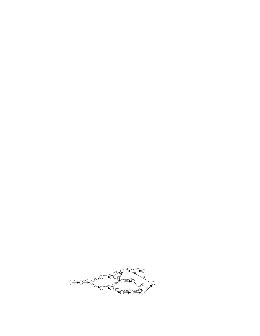
Figure 1: Slot-game semantics for the linear search with $k$=2

We show the model for this term with $k=2$ in Fig. 1. The worst-case cost of this term is equal to the array’s size $k$, which occurs when the search fails or the value of $h$ is compared with all elements of the array. We can perform a security analysis for this term by considering the model extended as in (7), where $m=0$. We obtain that this term has timing leaks, with a counter-example corresponding to two computations, such that initial values of $h$ are different, and the search succeeds in the one after only one iteration of $\mathsf{while}$ and fails in the other. For example, this will happen when all values in the array $x$ are 0’s, and the value of $h$ is 0 in the first computation and 1 in the second one.

We can also automatically analyse in an analogous way terms where the array size $k$ is much larger. Also the set of data that can be stored into the global variable $h$ and array $x$ can be larger than $\{0,1\}$. In these cases we will obtain models with much bigger number of states, but they still can be automatically analysed by calls to the FDR tool.

7 Conclusion

In this paper we have described how game semantics can be used for verifying security properties of open sequential programs, such as timing leaks and non-interference. This approach can be extended to terms with infinite data types, such as integers, by using some of the existing methods and tools based on game semantics for verifying such terms. Counter-example guided abstraction refinement procedure (ARP) [5] and symbolic representation of game semantics model [7] are two methods which can be used for this aim. The technical apparatus introduced here applies not only to time as a resource but to any other observable resource, such as power or heating of the processor. They can all be modeled in the framework of slot games and checked for information leaks.

We have focussed here on analysing the IA language, but we can easily extend this approach to any other language for which game semantics exists. Since fully abstract game semantics was also defined for probabilistic [4], concurrent [12], and programs with exceptions [1], it will be interesting to extend this approach to such programs.

References

- [1] Abramsky, S., and McCusker, G: Game Semantics. In Proceedings of the 1997 Marktoberdorf Summer School: Computational Logic , (1998), 1–56. Springer.
- [2] Agat, J: Transforming out Timing Leaks. In: Wegman, M.N., Reps, T.W. (eds.) POPL 2000. ACM, pp. 40–53. ACM, New York (2000), 10.1145/325694.325702.
- [3] Barthe, G., D’Argenio, P.R., Rezk, T: Secure information flow by self-composition. In: IEEE CSFW 2004. pp. 100–114. IEEE Computer Society Press, (2004), 10.1109/CSFW.2004.17.
- [4] V. Danos and R. Harmer. Probabilistic Game Semantics. In Proceedings of LICS 2000. 204–213. IEEE Computer Society Press, Los Alamitos (2000), 10.1109/LICS.2000.855770.
- [5] Dimovski, A., Ghica, D. R., Lazić, R. Data-Abstraction Refinement: A Game Semantic Approach. In: Hankin, C., Siveroni, I. (eds.) SAS 2005. LNCS vol. 3672, pp. 102–117. Springer, Heidelberg (2005), 10.1007/11547662 9.
- [6] Dimovski, A., Lazić, R: Compositional Software Verification Based on Game Semantics and Process Algebras. In Int. Journal on STTT 9(1), pp. 37–51, (2007), 10.1007/s10009-006-0005-y.
- [7] Dimovski, A: Symbolic Representation of Algorithmic Game Semantics. In: Faella, M., Murano, A. (eds.) GandALF 2012. EPTCS vol. 96, pp. 99–112. Open Publishing Association, (2012), 10.4204/EPTCS.96.8.
- [8] Dimovski, A: Ensuring Secure Non-interference of Programs by Game Semantics. Submitted for publication.
- [9] Cartwright, R., Curien, P. L., and Felleisen, M: Fully abstract semantics for observably sequential languages. In Information and Computation 111(2), pp. 297–401, (1994), 10.1006/inco.1994.1047.
- [10] Ghica, D. R., McCusker, G: The Regular-Language Semantics of Second-order Idealized Algol. Theoretical Computer Science 309 (1–3), pp. 469–502, (2003), 10.1016/S0304-3975(03)00315-3.
- [11] Ghica, D. R. Slot Games: a quantitative model of computation. In Palsberg, J., Abadi, M. (eds.) POPL 2005. ACM, pp. 85–97. ACM Press, New York (1998), 10.1145/1040305.1040313.
- [12] Ghica, D. R., Murawski, A: Compositional Model Extraction for Higher-Order Concurrent Programs. In: Hermanns, H., Palsberg, J. (eds.) TACAS 2006. LNCS vol. 3920, pp. 303–317. Springer, Heidelberg (2006), 10.1007/11691372 20.
- [13] Goguen, J., Meseguer, J: Security polices and security models. In: IEEE Symp. on Security and Privacy 1982. pp. 11–20. IEEE Computer Society Press, (1982).
- [14] Heintze, N., Riecke, J.G: The SLam calculus: programming with secrecy and integrity. In: MacQueen, D.B., Cardelli, L. (eds.) POPL 1998. ACM, pp. 365–377. ACM, New York (1998), 10.1145/268946.268976.
- [15] Joshi, R., and Leino, K.R.M: A semantic approach to secure information flow. In Science of Computer Programming 37, pp. 113–138, (2000), 10.1016/S0167-6423(99)00024-6.
- [16] Reynolds, J. C: The essence of Algol. In: O’Hearn, P.W, and Tennent, R.D. (eds), Algol-like languages. (Birkhaüser, 1997).
- [17] Roscoe, W. A: Theory and Practice of Concurrency. Prentice-Hall, 1998.
- [18] Sabelfeld, A., and Myers, A.C: Language-based information-flow security. In IEEE Journal on Selected Areas in Communications 21(1), (2003), 5–19, 10.1109/JSAC.2002.806121.
- [19] Sands, D: Improvement Theory and its Applications. Cambridge University Press, 1998.
- [20] Volpano, D., Smith, G., and Irvine, C: A sound type system for secure flow analysis. In Journal of Computer Security 4(2/3), (1996), 167–188, 10.3233/JCS-1996-42-304.
- [21] Volpano, D., Smith, G: Eliminating covert flows with minimum typings. In: IEEE Computer Security Foundations Workshop (CSFW), 1997, 156–169. IEEE Computer Society Press, (1997), 10.1109/CSFW.1997.596807.