High Precision Differential Abundance Measurements in Globular Clusters: Chemical Inhomogeneities in NGC 6752

Abstract

We report on a strictly differential line-by-line analysis of high quality UVES spectra of bright giants in the metal-poor globular cluster NGC 6752. We achieved high precision differential chemical abundance measurements for Fe, Na, Si, Ca, Ti, Cr, Ni, Zn, Y, Zr, Ba, La, Ce, Pr, Nd, Sm, Eu and Dy with uncertainties as low as $\sim$0.01 dex ($\sim$2%). We obtained the following main results. (1) The observed abundance dispersions are a factor of $\sim$2 larger than the average measurement uncertainty. (2) There are positive correlations, of high statistical significance, between all elements and Na. (3) For any pair of elements, there are positive correlations of high statistical significance, although the amplitudes of the abundance variations are small. Removing abundance trends with effective temperature and/or using a different pair of reference stars does not alter these results. These abundance variations and correlations may reflect a combination of ($a$) He abundance variations and $(b)$ inhomogeneous chemical evolution in the pre- or proto-cluster environment. Regarding the former, the current constraints on $\Delta Y$ from photometry likely preclude He as being the sole explanation. Regarding the latter, the nucleosynthetic source(s) must have synthesised Na, $\alpha$, Fe-peak and neutron-capture elements and in constant amounts for species heavier than Si; no individual object can achieve such nucleosynthesis. We speculate that other, if not all, globular clusters may exhibit comparable abundance variations and correlations to NGC 6752 if subjected to a similarly precise analysis.

1 Introduction

Understanding the origin of the star-to-star abundance variations of the light elements in globular clusters is one of the major challenges confronting stellar evolution, stellar nucleosynthesis and chemical evolution. Arguably the first evidence for chemical abundance inhomogeneity in a globular cluster was the discovery of a CN strong star in M13 by Popper (1947). A large number of subsequent studies have confirmed the star-to-star variation in the strength of the CN molecular bands in a given globular cluster, and these results have been extended to star-to-star abundance variations for the light elements – Li, C, N, O, F, Na, Mg and Al (e.g., see reviews by Smith 1987, Kraft 1994 and Gratton et al. 2004, 2012). In light of the discovery of abundance variations in unevolved stars (e.g., Cannon et al. 1998; Gratton et al. 2001; Ramírez & Cohen 2002, 2003), the consensus view is that these light element abundance variations are attributed to a proto-cluster environment in which the gas was of an inhomogeneous composition. The interstellar medium from which some of the stars formed included material processed through hydrogen-burning at high temperatures. The source of that material and the nature of the nucleosynthesis, however, remain highly contentious with intermediate-mass asymptotic giant branch stars, fast rotating massive stars and massive binaries being the leading candidates (e.g., Fenner et al. 2004, Ventura & D’Antona 2005, Decressin et al. 2007, de Mink et al. 2009, Marcolini et al. 2009).

Recent discoveries of complex structure in colour-magnitude diagrams reveal that most, if not all, globular clusters host multiple populations; the evidence consists of multiple main sequences, subgiant branches, red giant branches and/or horizontal branches in Galactic (e.g., see Piotto 2009 for a review) and also extragalactic globular clusters (e.g., Mackey & Broby Nielsen 2007; Milone et al. 2009). When using appropriate photometric filters, all globular clusters show well-defined sequences with distinct chemical abundance patterns (Milone et al., 2012). These multiple populations can be best explained by different ages and/or chemical compositions. The sequence of events leading to the formation of multiple population globular clusters is not well understood (e.g., D’Ercole et al. 2008; Bekki 2011; Conroy & Spergel 2011).

Although the census and characterization of the Galactic globular clusters remains incomplete, they may be placed into three general categories: ($i$) those that exhibit only light element abundance variations, which include NGC 6397, NGC 6752 and 47 Tuc (e.g., Gratton et al. 2001; Yong et al. 2005; D’Orazi et al. 2010; Lind et al. 2011b; Campbell et al. 2013), ($ii$) those that exhibit light element abundance variations and neutron-capture element abundance dispersions such as M15 (e.g., Sneden et al. 1997, 2000; Sobeck et al. 2011) and ($iii$) those that exhibit light element abundance variations as well as significant abundance dispersions for Fe-peak elements such as $\omega$ Cen, M22, M54, NGC 1851, NGC 3201 and Terzan 5 (e.g., Norris & Da Costa 1995; Yong & Grundahl 2008; Marino et al. 2009, 2011; Carretta et al. 2010; Johnson & Pilachowski 2010; Villanova et al. 2010; Carretta et al. 2011; Origlia et al. 2011; Roederer et al. 2011; Alves-Brito et al. 2012; Simmerer et al. 2013). At this stage, we do not attempt to classify a particularly unusual system like NGC 2419 (Cohen et al., 2010, 2011; Cohen & Kirby, 2012; Mucciarelli et al., 2012).

Given the surprisingly large star-to-star variations in element abundance ratios in a given cluster, how chemically homogeneous are the “well-behaved” elements in the ”normal” globular clusters (i.e., clusters in category ($i$) above)? The answer to this question has important consequences for testing model predictions, setting constraints on the polluters and understanding the origin and evolution of globular clusters.

Sneden (2005) considered the issue of cluster abundance accuracy limits and selected the [Ni/Fe] ratio as an example. This pair of elements was chosen as they present numerous spectral lines in the “uncomplicated yellow-red region” of the spectrum and share “common nucleosynthetic origins in supernovae”. Sneden (2005) noted that the dispersion in the [Ni/Fe] ratio in a cluster was $\sim$0.06 dex and appeared to show “little apparent trend as a function of the number of stars observed in a survey or of year of publication”. There are two possible reasons for the apparent limit in the $\sigma$[Ni/Fe] ratio. Perhaps clusters possess a single [Ni/Fe] ratio and the dispersion reflects the measurement uncertainties. Alternatively, globular clusters are chemically homogeneous in the [Ni/Fe] ratio at the $\sim$0.06 dex level. Bearing in mind this apparent limit in the [Ni/Fe] dispersion, in order to answer the question posed above, we require the highest possible precision when measuring chemical abundances.

A number of recent studies have achieved precision in chemical abundance measurements as low as 0.01 dex (e.g., Meléndez et al. 2009, 2012, Alves-Brito et al. 2010, Nissen & Schuster 2010, 2011, Ramírez et al. 2010, 2012). These results were obtained by using ($i$) high quality spectra (R $\geq$ 60,000 and signal-to-noise ratios S/N $\geq$ 200 per pixel), ($ii$) a strictly differential line-by-line analysis and ($iii$) a well-chosen sample of stars covering a small range in stellar parameters (effective temperature, surface gravity, metallicity). Application of similar analysis techniques to high quality spectra of stars in globular clusters offers the hope that high precision chemical abundance measurements (at the $\sim$0.01 dex level) can also be obtained. To our knowledge, the highest precision chemical abundance measurements in globular clusters to date are at the $\sim$0.04 dex level include Yong et al. (2005), Gratton et al. (2005), Carretta et al. (2009a) and Meléndez & Cohen (2009). The aim of the present paper is to achieve high precision abundance measurements in the globular cluster NGC 6752 and to use these data to study the chemical enrichment history of this cluster.

2 OBSERVATIONS AND ANALYSIS

2.1 Target Selection and Spectroscopic Observations

The targets for this study were taken from the $uvby$ photometry by Grundahl et al. (1999). The sample consists of 17 stars located near the tip of the red giant branch (hereafter RGB tip stars) and 21 stars located at the bump in the luminosity function along the RGB (hereafter RGB bump stars). The list of targets can be found in Table 1. Observations were performed using the Ultraviolet and Visual Echelle Spectrograph (UVES; Dekker et al. 2000) on the 8.2m Kueyen (VLT/UT2) telescope at Cerro Paranal, Chile. The RGB tip stars were observed at a resolving power of R = 110,000 and S/N $\geq$ 150 per pixel near 5140Å while the RGB bump stars were observed at R = 60,000 and S/N $\geq$ 100 per pixel near 5140Å. Analyses of these spectra have been reported in Grundahl et al. (2002) and Yong et al. (2003, 2005, 2008). The location of the program stars in a colour-magnitude diagram can be found in Figure 1 in Yong et al. (2003).

Table 1: Program Stars and Stellar Parameters as Defined in Section 2.3.

Name1	Name2	RA2000	DE2000	$V$	$T_{\rm eff}$	$\log g$b	$\xi_{t}$b	[Fe/H]b
					(K)	(cm s-2)	(km s-1)
(1)	(2)	(3)	(4)	(5)	(6)	(7)	(8)	(9)
PD1	NGC6752-mg0	19:10:58	$-$59:58:07	10.70	3928	0.26	2.20	$-$1.67
B1630	NGC6752-mg1	19:11:11	$-$59:59:51	10.73	3900	0.24	2.25	$-$1.70
B3589	NGC6752-mg2	19:10:32	$-$59:57:01	10.94	3894	0.33	2.07	$-$1.66
B1416	NGC6752-mg3	19:11:17	$-$60:03:10	10.99	4050	0.50	1.88	$-$1.66
…	NGC6752-mg4	19:10:43	$-$59:59:54	11.02	4065	0.53	1.86	$-$1.65
PD2	NGC6752-mg5	19:10:49	$-$59:59:34	11.03	4100	0.56	1.90	$-$1.65
B2113	NGC6752-mg6	19:11:03	$-$60:01:43	11.22	4154	0.68	1.85	$-$1.62
…	NGC6752-mg8	19:10:38	$-$60:04:10	11.47	4250	0.80	1.71	$-$1.69
B3169	NGC6752-mg9	19:10:40	$-$59:58:14	11.52	4288	0.91	1.72	$-$1.66
B2575	NGC6752-mg10	19:10:54	$-$59:57:14	11.54	4264	0.90	1.66	$-$1.67
…	NGC6752-mg12	19:10:58	$-$59:57:04	11.59	4286	0.94	1.73	$-$1.68
B2196	NGC6752-mg15	19:11:01	$-$59:57:18	11.68	4354	1.02	1.74	$-$1.64
B1518	NGC6752-mg18	19:11:15	$-$60:00:29	11.83	4398	1.11	1.68	$-$1.64
B3805	NGC6752-mg21	19:10:28	$-$59:59:49	11.99	4429	1.20	1.68	$-$1.65
B2580	NGC6752-mg22	19:10:54	$-$60:02:05	11.99	4436	1.20	1.71	$-$1.65
B1285	NGC6752-mg24	19:11:19	$-$60:00:31	12.15	4511	1.31	1.69	$-$1.67
B2892	NGC6752-mg25	19:10:46	$-$59:56:22	12.23	4489	1.33	1.70	$-$1.67
…	NGC6752-0	19:11:03	$-$59:59:32	13.03	4699	1.83	1.43	$-$1.66
B2882	NGC6752-1	19:10:47	$-$60:00:43	13.27	4749	1.95	1.37	$-$1.63
B1635	NGC6752-2	19:11:11	$-$60:00:17	13.30	4779	1.98	1.37	$-$1.63
B2271	NGC6752-3	19:11:00	$-$59:56:40	13.41	4796	2.03	1.38	$-$1.69
B611	NGC6752-4	19:11:33	$-$60:00:02	13.42	4806	2.04	1.38	$-$1.65
B3490	NGC6752-6	19:10:34	$-$59:59:55	13.47	4804	2.06	1.33	$-$1.64
B2438	NGC6752-7	19:10:57	$-$60:00:41	13.53	4829	2.10	1.32	$-$1.86
B3103	NGC6752-8	19:10:45	$-$59:58:18	13.56	4910	2.15	1.33	$-$1.69
B3880	NGC6752-9	19:10:26	$-$59:59:05	13.57	4824	2.11	1.41	$-$1.70
B1330	NGC6752-10	19:11:18	$-$59:59:42	13.60	4836	2.13	1.37	$-$1.65
B2728	NGC6752-11	19:10:50	$-$60:02:25	13.62	4829	2.13	1.34	$-$1.68
B4216	NGC6752-12	19:10:20	$-$60:00:30	13.64	4841	2.15	1.35	$-$1.66
B2782	NGC6752-15	19:10:49	$-$60:01:55	13.73	4850	2.19	1.36	$-$1.63
B4446	NGC6752-16	19:10:15	$-$59:59:14	13.78	4906	2.24	1.33	$-$1.63
B1113	NGC6752-19	19:11:23	$-$59:59:40	13.96	4928	2.32	1.33	$-$1.68
…	NGC6752-20	19:10:36	$-$59:56:08	13.98	4929	2.33	1.32	$-$1.63
…	NGC6752-21	19:11:13	$-$60:02:30	14.02	4904	2.33	1.31	$-$1.67
B1668	NGC6752-23	19:11:12	$-$59:58:29	14.06	4916	2.35	1.25	$-$1.66
…	NGC6752-24	19:10:44	$-$59:59:41	14.06	4948	2.37	1.16	$-$1.71
…	NGC6752-29	19:10:17	$-$60:01:00	14.18	4950	2.42	1.31	$-$1.69
…	NGC6752-30	19:10:39	$-$59:59:47	14.19	4943	2.42	1.26	$-$1.64

Based on multi-band Hubble Space Telescope (HST) and ground-based Strömgren photometry, Milone et al. (2013) have identified three populations on the main sequence, subgiant branch and red giant branch of NGC 6752. These populations, which we refer to as $a$, $b$ and $c$, exhibit distinct chemical abundance patterns: population $a$ has a chemical composition similar to that of field halo stars (e.g., high O and low Na); population $c$ is enhanced in N, Na and He ($\Delta Y\sim 0.03)$ and depleted C and O; population $b$ has a chemical composition intermediate between populations $a$ and $c$ with slightly enhanced He ($\Delta Y\sim 0.01)$. Using the data from Milone et al. (2013), we can classify all program stars according to their populations. In the relevant figures, stars of populations $a$, $b$ and $c$ are coloured green, magenta and blue, respectively.

2.2 Line List and Equivalent Width Measurements

The first step in our analysis was to measure equivalent widths (EWs) for a large set of lines. The line list was taken primarily from Gratton et al. (2003) and supplemented with laboratory measurements for Fe i from the Oxford group (Blackwell et al., 1979a, b, 1980, 1986, 1995), laboratory measurements for Fe ii from Biemont et al. (1991) and for various elements, the values taken from the references listed in Yong et al. (2005) (which are also listed in Tables 2 and 3). We used the DAOSPEC (Stetson & Pancino, 2008) software package to measure EWs in our program stars. For the subset of lines we had previously measured using routines in IRAF, we compared those values with the DAOSPEC measurements and found excellent agreement between the two sets of EW measurements for lines having strengths less than $\sim$100mÅ (see Figure 1). For the 1,542 lines with EW $<$ 100 mÅ, we find a mean difference EW(DY) $-$ EW(DAOSPEC) = 1.14 $\pm$ 0.05 mÅ ($\sigma$ = 1.92 mÅ). For our analysis, we adopted only lines with 5 mÅ $<$ EW $<$ 100 mÅ as measured by DAOSPEC. A further requirement was that a given line must be measured in every RGB tip star or every RGB bump star. That is, the line list for the RGB tip sample was different from the line list for the RGB bump sample, but for either sample of stars, each line was measured in every star within a particular sample. Due to the lower quality spectra for the RGB bump sample, we required lines to have EW $\geq$ 10 mÅ. The line list and EW measurements for the RGB tip sample and for the RGB bump sample are presented in Tables 2 and 3, respectively.

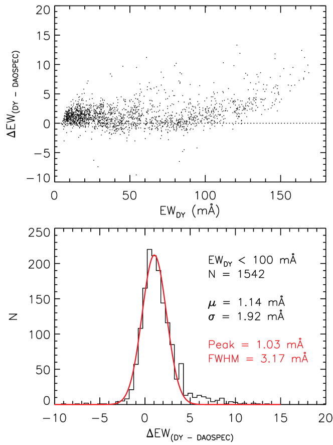
Figure 1: Comparison of EWs measured using IRAF (DY) and DAOSPEC. The upper panel shows all lines (N = 1,795). The lower panel shows the distribution of the EW differences for the 1,542 lines with EW_DY $<$ 100 mÅ (i.e., measured using IRAF). We superimpose the Gaussian fit to the distribution and write the relevant parameters associated with the fit as well as the mean and dispersion.

Table 2: Line List for the RGB Tip Stars

Wavelength	Species	L.E.P	$\log gf$	mg0	mg1	mg2	mg3	mg4	Source
Å		eV		mÅ	mÅ	mÅ	mÅ	mÅ
(1)	(2)	(3)	(4)	(5)	(6)	(7)	(8)	(9)	(10)
6154.23	11.0	2.10	$-$1.56	48.2	32.2	23.9	18.5	20.3	A
6160.75	11.0	2.10	$-$1.26	74.7	53.1	42.1	34.2	37.7	A
5645.61	14.0	4.93	$-$2.14	16.0	16.3	15.8	15.6	15.9	A
5665.56	14.0	4.92	$-$2.04	20.3	20.4	20.4	19.4	19.4	B
5684.49	14.0	4.95	$-$1.65	35.0	36.1	34.2	34.1	33.3	B

This table is published in its entirety in the electronic edition of the MNRAS. A portion is shown here for guidance regarding its form and content.

Table 3: Line List for the RGB Bump Stars.

Wavelength	Species	L.E.P	$\log gf$	0	1	2	3	4	Source
Å		eV		mÅ	mÅ	mÅ	mÅ	mÅ
(1)	(2)	(3)	(4)	(5)	(6)	(7)	(8)	(9)	(10)
5682.65	11.0	2.10	$-$0.71	52.1	18.6	56.1	15.3	50.2	A
5688.22	11.0	2.10	$-$0.40	77.0	31.9	75.5	27.3	73.8	A
5684.49	14.0	4.95	$-$1.65	24.4	22.9	22.5	20.8	23.6	B
5708.40	14.0	4.95	$-$1.47	38.3	28.7	33.9	28.4	30.4	B
5948.55	14.0	5.08	$-$1.23	43.5	36.9	39.4	31.8	37.5	A

This table is published in its entirety in the electronic edition of the MNRAS. A portion is shown here for guidance regarding its form and content.

2.3 Establishing Parameters for Reference Stars

In order to conduct the line-by-line strictly differential analysis, we needed to adopt a reference star. The reference star parameters were determined in the following manner. Note that since we did not know which reference stars would be adopted, the procedure was applied to all stars. Following our previous analyses of these spectra, effective temperatures, $T_{\rm eff}$, were derived from the Grundahl et al. (1999) $uvby$ photometry using the Alonso et al. (1999) $T_{\rm eff}$:colour:[Fe/H] relations. Surface gravities, $\log g$, were estimated using $T_{\rm eff}$ and the stellar luminosity. The latter value was determined by assuming a mass of 0.84 M_⊙, a reddening $E(B-V)$ = 0.04 (Harris, 1996) and bolometric corrections taken from a 14 Gyr isochrone with [Fe/H] = $-$1.54 from VandenBerg et al. (2000).

The model atmospheres used in the analysis were the one-dimensional, plane-parallel, local thermodynamic equilibrium (LTE), $\alpha$-enhanced, [$\alpha$/Fe] = +0.4, NEWODF grid of ATLAS9 models by Castelli & Kurucz (2003). We used linear interpolation software (written by Dr Carlos Allende Prieto and tested in Allende Prieto et al. 2004) to produce a particular model. (See Mészáros & Allende Prieto 2013 for a discussion of interpolation of model atmospheres.) Using the 2011 version of the stellar line analysis program MOOG (Sneden, 1973; Sobeck et al., 2011), we computed the abundance for a given line. The microturbulent velocity, $\xi_{t}$, was set, in the usual way, by forcing the abundances from Fe i lines to have zero slope against the reduced equivalent width, EW_r = $\log(W_{\lambda}/\lambda)$. The metallicity was inferred from Fe i lines. We iterated this process until the inferred metallicity matched the value adopted to generate the model atmosphere (this process usually converged within three iterations). (We exclude the RGB bump star NGC 6752-7 (B2438) due to its discrepant iron abundance, most likely resulting from a photometric blend which affected the $T_{\rm eff}$ and $\log g$ values.)

2.4 Line-by-line Strictly Differential Stellar Parameters

Following Meléndez et al. (2012), we determined the stellar parameters using a strictly differential line-by-line analysis between the program stars and a reference star. Given the difference in $T_{\rm eff}$ between the RGB tip and RGB bump samples, we treated each sample separately.

For the RGB tip stars, we selected NGC 6752-mg9 to be the reference star since it had a $T_{\rm eff}$ value close to the median for the RGB tip stars and the O/Na/Mg/Al abundances were also close to the median values. These decisions were motivated by the expectation that the errors in the derived stellar parameters, and therefore errors in the chemical abundances, would increase if there was a large difference in $T_{\rm eff}$ between the program star and the reference star. Thus, we selected a star with $T_{\rm eff}$ close to the median value to minimise the difference in $T_{\rm eff}$ between the program stars and the reference star. Similarly, we were concerned that large differences in the abundances of O/Na/Mg/Al between the program star and the reference star could increase the errors in the derived stellar parameters and chemical abundances. Again, selecting the reference star to have O/Na/Mg/Al abundances close to the median value minimises the abundance differences between the program stars and the reference star. Application of a similar approach to the RGB bump sample resulted in the selection of NGC 6752-11 as the reference star.

To determine the stellar parameters for a program star, we generated a model atmosphere with a particular combination of effective temperature ($T_{\rm eff}$), surface gravity ($\log g$), microturbulent velocity ($\xi_{t}$) and metallicity, [m/H]. The initial guesses for these parameters came from the values in Section 2.3. Using MOOG, we computed the abundances for Fe i and Fe ii lines. We then examined the line-by-line Fe abundance differences. Adopting the notation from Meléndez et al. (2012), the abundance difference (program star $-$ reference star) for a line is

$$\delta A_{i}=A_{i}^{\rm program~{}star}-A_{i}^{\rm reference~{}star}.$$ (1)

We examined the abundance differences for Fe i as a function of lower excitation potential. We forced excitation equilibrium by imposing the following constraint

$$\frac{\partial(\delta A_{i}^{\rm FeI})}{\partial(\chi_{\rm exc})}=0.$$ (2)

Next, we considered the abundance differences for Fe i as a function of reduced equivalent width, EW_r, and imposed the following constraint

$$\frac{\partial(\delta A_{i}^{\rm FeI})}{\partial({\rm EW}_{r})}=0.$$ (3)

For any species, Fe i in this example, we then defined the average abundance difference as

$$\Delta^{\rm FeI}=\langle\delta A_{i}^{\rm FeI}\rangle=\frac{1}{N}\sum\limits_{i=1}^{N}\delta A_{i}^{\rm FeI}$$ (4)

Similarly, we defined the average Fe ii abundance as $\Delta^{\rm FeII}$ = $\langle\delta A_{i}^{\rm FeII}\rangle$, and the relative ionization equilibrium as

$$\Delta^{\rm FeI-FeII}=\Delta^{\rm FeI}-\Delta^{\rm FeII}=\langle\delta A_{i}^{\rm FeI}\rangle-\langle\delta A_{i}^{\rm FeII}\rangle=0.$$ (5)

Unlike Meléndez et al. (2012), we did not take into account the relative ionization equilibria for Cr and Ti, nor did we consider non-LTE effects for any species. We note that while departures from LTE are expected for Fe i for metal-poor giants (Lind et al., 2012), the relative non-LTE effects across our range of stellar parameters are vanishingly small.

The final stellar parameters for a program star were obtained when equations (2), (3) and (5) were simultaneously satisfied and the derived metallicity was identical to that used in generating the model atmosphere. Regarding the latter criterion, we provide the following example. The metallicity of the reference star NGC 6752-mg9 was [Fe/H] = $-$1.66 when adopting the Asplund et al. (2009) solar abundances and the photometric stellar parameters described in Section 2.3 (see Table 1). For star NGC 6752-mg8, the average abundance difference for Fe i, and also Fe ii given equation (5), was $\langle\delta A_{i}^{\rm FeI}\rangle$ = +0.01 dex. Thus, the stellar parameters can only be regarded as final if equations (2), (3) and (5) are satisfied and the model atmosphere is generated assuming a global metallicity of [m/H] = [Fe/H]_NGC6752-mg9 + $\langle\delta A_{i}^{\rm FeI}\rangle$ = $-$1.65.

While equations (2), (3) and (5) are primarily sensitive to $T_{\rm eff}$, $\xi_{t}$ and $\log g$, respectively, in practice, all three equations are affected by small changes in any stellar parameter. Derivation of these strictly differential stellar parameters required multiple iterations (up to 20) where each iteration selected a single value for [m/H] and five values for each parameter, $T_{\rm eff}$, $\log g$ and $\xi_{t}$, in steps of 5 K, 0.05 dex and 0.05 km s^-1, respectively, i.e., 125 models per iteration. We then examined the output from the 125 models to see whether equations (2), (3) and (5) were simultaneously satisfied and whether the derived metallicity matched that of the model atmosphere. If not, the best model was identified and we repeated the process. If so, we conducted a final iteration in which we selected a single value for [m/H] and tested 11 values for each parameter, $T_{\rm eff}$, $\log g$ and $\xi_{t}$, in steps of 1 K, 0.01 dex and 0.01 km s^-1, respectively, i.e., 1,331 models in the final iteration using a smaller step size for each parameter, and the best model was selected. As noted, this process was performed separately for the RGB tip sample and for the RGB bump sample. The strictly differential stellar parameters obtained using this pair of reference stars (RGB tip = NGC 6752-mg9, RGB bump = NGC 6752-11) are presented in Table 4. (We exclude the RGB tip star NGC 6752-mg1 because the stellar parameters did not converge. Specifically, the best solution required a value for $\log g$ beyond the boundary of the Castelli & Kurucz (2003) grid of model atmospheres.) Figures 2 and 3 provide examples of $\delta A_{i}$, for Fe i and Fe ii, versus lower excitation potential and reduced EW for the strictly differential stellar parameters for a representative RGB tip star and a representative RGB bump star, respectively. That is, these figures show the results when equations (2), (3) and (5) are simultaneously satisfied and the derived metallicity is the same as that used to generate the model atmosphere.

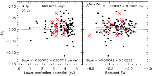
Figure 2: Abundance differences, $\delta A_{i}$, for the RGB tip star NGC6752-mg8 (reference star NGC 6752-mg9) versus lower excitation potential (left) and reduced EW (right). Values for Fe i and Fe ii are shown as black squares and red crosses, respectively. The blue dashed line in each panel is the linear least squares fit to the data and we write the slope and associated uncertainty in each panel. In the right panel, we also write $\Delta^{\rm FeI-FeII}=\langle\delta A_{i}^{\rm FeI}\rangle-\langle\delta A_{i}^{\rm FeII}\rangle$.

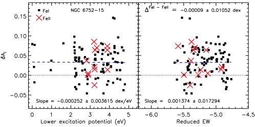
Figure 3: Same as Figure 2 but for the RGB bump star NGC 6752-15 (reference star NGC 6752-11).

Table 4: Strictly Differential Stellar Parameters, and Uncertainties, When Adopting the First Set of Reference Stars (RGB Tip = NGC 6752-mg9, RGB Bump = NGC 6752-11).

Name	$T_{\rm eff}$	$\sigma$	$\log g$	$\sigma$	$\xi_{t}$	$\sigma$	[Fe/H]
	(K)	(K)	(cm s-2)	(cm s-2)	(km s-1)	(km s-1)
(1)	(2)	(3)	(4)	(5)	(6)	(7)	(8)
NGC6752-mg0	3919	20	0.16	0.01	2.24	0.05	$-$1.69
NGC6752-mg2	3938	22	0.23	0.01	2.13	0.05	$-$1.67
NGC6752-mg3	4066	19	0.53	0.01	1.93	0.04	$-$1.65
NGC6752-mg4	4081	18	0.54	0.01	1.90	0.04	$-$1.65
NGC6752-mg5	4100	17	0.56	0.01	1.93	0.04	$-$1.66
NGC6752-mg6	4151	19	0.65	0.01	1.88	0.04	$-$1.63
NGC6752-mg8	4284	14	0.93	0.01	1.73	0.04	$-$1.65
NGC6752-mg10	4291	12	0.92	0.01	1.70	0.03	$-$1.66
NGC6752-mg12	4315	13	0.96	0.01	1.76	0.04	$-$1.66
NGC6752-mg15	4339	13	1.01	0.01	1.76	0.04	$-$1.66
NGC6752-mg18	4380	15	1.07	0.01	1.71	0.04	$-$1.66
NGC6752-mg21	4437	13	1.16	0.01	1.69	0.05	$-$1.65
NGC6752-mg22	4444	14	1.19	0.01	1.71	0.04	$-$1.64
NGC6752-mg24	4505	17	1.30	0.01	1.72	0.07	$-$1.68
NGC6752-mg25	4471	15	1.24	0.01	1.74	0.07	$-$1.69
NGC6752-0	4706	12	1.85	0.01	1.44	0.02	$-$1.65
NGC6752-1	4719	11	1.94	0.01	1.37	0.02	$-$1.65
NGC6752-2	4739	12	1.95	0.01	1.35	0.02	$-$1.66
NGC6752-3	4749	13	2.00	0.01	1.34	0.02	$-$1.73
NGC6752-4	4794	13	2.08	0.01	1.37	0.02	$-$1.66
NGC6752-6	4795	11	2.10	0.01	1.32	0.02	$-$1.64
NGC6752-8	4930	15	2.29	0.01	1.31	0.03	$-$1.67
NGC6752-9	4795	21	2.09	0.01	1.40	0.04	$-$1.73
NGC6752-10	4811	10	2.11	0.01	1.35	0.02	$-$1.67
NGC6752-12	4822	13	2.15	0.01	1.34	0.02	$-$1.68
NGC6752-15	4830	12	2.23	0.01	1.34	0.02	$-$1.65
NGC6752-16	4875	15	2.24	0.01	1.31	0.03	$-$1.66
NGC6752-19	4892	12	2.32	0.01	1.31	0.02	$-$1.71
NGC6752-20	4899	12	2.32	0.01	1.30	0.02	$-$1.65
NGC6752-21	4884	14	2.32	0.01	1.30	0.03	$-$1.69
NGC6752-23	4912	12	2.33	0.01	1.25	0.02	$-$1.67
NGC6752-24	4911	17	2.39	0.01	1.14	0.03	$-$1.74
NGC6752-29	4923	13	2.40	0.01	1.30	0.02	$-$1.71
NGC6752-30	4919	12	2.47	0.01	1.24	0.02	$-$1.66

In Figures 4 and 5 we compare the “reference star” stellar parameters (described in Sec 2.3) and the “strictly differential” stellar parameters (described above) for the RGB tip and RGB bump samples, respectively, using the reference stars noted above. For the RGB tip sample, the average difference between the “reference star” and “strictly differential” values for $T_{\rm eff}$, $\log g$, $\xi_{t}$ and [Fe/H] are very small; 7.53 K $\pm$ 5.09 K, $-$0.015 dex (cgs) $\pm$ 0.015 dex (cgs), 0.031 km s^-1 $\pm$ 0.004 km s^-1 and $-$0.002 dex $\pm$ 0.004 dex, respectively. Comparably small differences in stellar parameters are obtained for the RGB bump sample. Therefore, an essential point we make here is that the strictly differential stellar parameters do not involve any substantial change for any parameter, relative to the “reference star” stellar parameters. For $T_{\rm eff}$, the changes are within the uncertainties of the photometry.

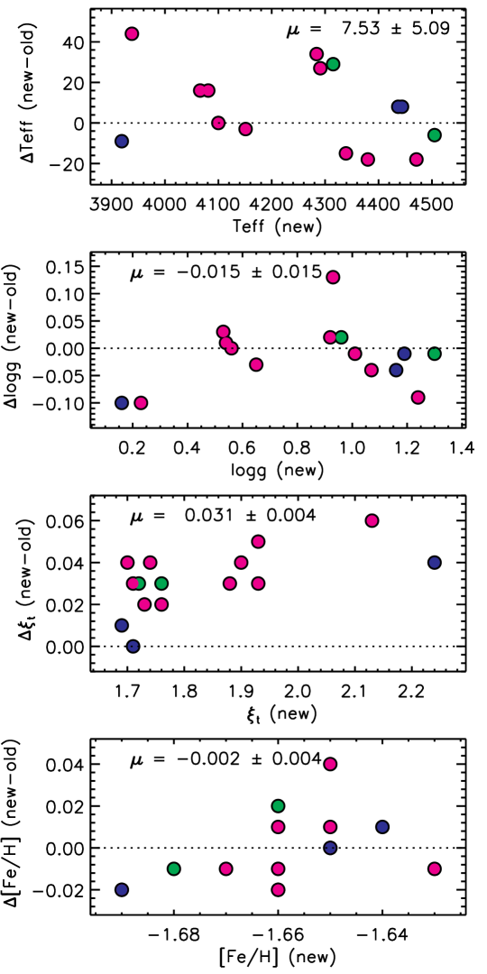
Figure 4: Differences in $T_{\rm eff}$, $\log g$, $\xi_{t}$ and [Fe/H] between the “reference star” (old) and the “strictly differential” (new) stellar parameters for the RGB tip sample (reference star is NGC 6752-mg9). The mean difference is written in each panel. The green, magenta and blue colours represent populations $a$, $b$ and $c$ from Milone et al. (2013) (see Section 2.1 for details).

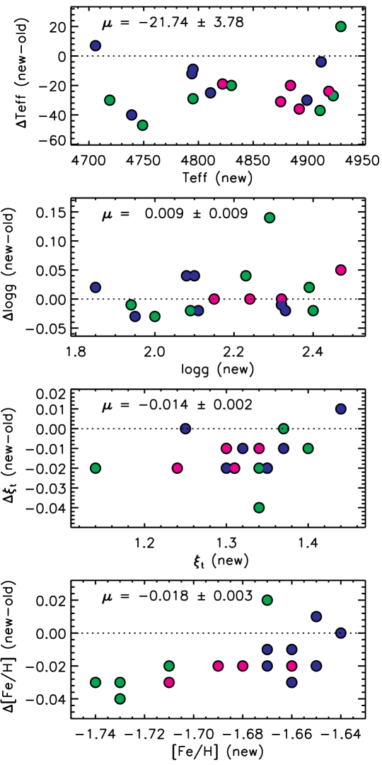
Figure 5: Same as Figure 4 but for the RGB bump sample (reference star is NGC 6752-11).

2.5 Chemical Abundances

Having obtained the strictly differential stellar parameters, we computed the abundances for the following species in every program star; Na, Si, Ca, Ti i, Ti ii, Cr i, Cr ii, Ni, Y, La, Nd and Eu. For the elements La and Eu, we used spectrum synthesis and $\chi^{2}$ analysis of the 5380Å and 6645Å lines, respectively, rather than an EW analysis since these lines are affected by hyperfine splitting (HFS) and/or isotope shifts. We treated these lines appropriately using the data from Kurucz & Bell (1995) and for Eu, we adopted the Lodders (2003) solar isotope ratios. The $\log gf$ values for the La and Eu lines were taken from Lawler et al. (2001a) and Lawler et al. (2001b), respectively.

We used equation (1) to obtain the abundance difference (between the program star and the reference star) for any line. For a particular species, X, the average abundance difference is $\langle\delta A_{i}^{\rm X}\rangle$ which we write as $\Delta^{\rm X}$, i.e., as defined in equation (4) above. In Tables 5 and 6, we present the abundance differences for each element in all program stars. In order to put these abundance differences onto an absolute scale, in these tables we also provide the A(X) abundances for the reference stars when using the stellar parameters in Table 1. The new [X/Fe] values are in very good agreement with our previously published values (Grundahl et al., 2002; Yong et al., 2003, 2005), although we have not attempted to reconcile the two sets of abundances.

Table 5: Differential Abundances (Fe, Na, Si, Ca and Ti) When Adopting the First Set of Reference Stars (RGB Tip = NGC 6752-mg9, RGB Bump = NGC 6752-11).

Star	$\Delta^{\rm Fe}$	$\sigma$	$\Delta^{\rm Na}$	$\sigma$	$\Delta^{\rm Si}$	$\sigma$	$\Delta^{\rm Ca}$	$\sigma$	$\Delta^{\rm TiI}$	$\sigma$	$\Delta^{\rm TiII}$	$\sigma$
(1)	(2)	(3)	(4)	(5)	(6)	(7)	(8)	(9)	(10)	(11)	(12)	(13)
NGC6752-mg0	$-$0.029	0.010	0.387	0.016	0.038	0.015	$-$0.023	0.033	0.021	0.020	$-$0.024	0.035
NGC6752-mg2	$-$0.011	0.011	$-$0.014	0.008	0.039	0.010	$-$0.021	0.049	0.050	0.024	0.036	0.039
NGC6752-mg3	0.007	0.015	$-$0.027	0.005	0.007	0.009	$-$0.003	0.045	0.020	0.017	0.043	0.041
NGC6752-mg4	0.010	0.014	0.041	0.010	0.030	0.010	0.008	0.038	0.023	0.012	0.043	0.045
NGC6752-mg5	0.005	0.008	0.052	0.008	0.015	0.008	0.001	0.015	0.006	0.012	0.038	0.035
NGC6752-mg6	0.032	0.009	$-$0.123	0.002	0.042	0.009	0.049	0.040	0.052	0.011	0.095	0.065
NGC6752-mg8	0.007	0.010	0.036	0.015	$-$0.001	0.017	0.004	0.024	0.008	0.023	0.029	0.019
NGC6752-mg10	0.007	0.010	0.013	0.004	$-$0.004	0.007	$-$0.005	0.017	$-$0.023	0.010	0.027	0.033
NGC6752-mg12	0.002	0.010	$-$0.342	0.004	$-$0.021	0.007	$-$0.017	0.016	0.006	0.007	$-$0.007	0.030
NGC6752-mg15	$-$0.001	0.009	0.044	0.009	$-$0.008	0.010	$-$0.008	0.011	$-$0.009	0.007	0.009	0.023
NGC6752-mg18	$-$0.002	0.010	$-$0.094	0.004	$-$0.006	0.009	$-$0.016	0.017	$-$0.018	0.007	0.044	0.033
NGC6752-mg21	0.018	0.009	0.282	0.009	0.043	0.009	0.032	0.013	$-$0.012	0.009	0.057	0.031
NGC6752-mg22	0.014	0.009	0.323	0.008	0.030	0.010	0.017	0.011	$-$0.012	0.010	0.012	0.031
NGC6752-mg24	$-$0.023	0.016	$-$0.345	0.035	$-$0.049	0.009	$-$0.040	0.012	$-$0.034	0.009	0.047	0.059
NGC6752-mg25	$-$0.027	0.010	$-$0.139	0.025	$-$0.008	0.010	$-$0.026	0.023	$-$0.045	0.009	$-$0.023	0.039
NGC6752-0	0.030	0.010	0.335	0.033	0.096	0.019	0.050	0.010	0.023	0.011	0.052	0.012
NGC6752-1	0.025	0.009	$-$0.366	0.020	$-$0.008	0.013	0.031	0.010	0.003	0.011	0.034	0.012
NGC6752-2	0.020	0.008	0.384	0.015	0.055	0.012	0.038	0.008	$-$0.001	0.008	0.031	0.014
NGC6752-3	$-$0.049	0.012	$-$0.444	0.016	$-$0.044	0.007	$-$0.044	0.009	$-$0.052	0.013	$-$0.036	0.017
NGC6752-4	0.017	0.015	0.352	0.021	0.026	0.021	0.065	0.011	0.007	0.013	0.034	0.017
NGC6752-6	0.036	0.014	0.262	0.017	0.032	0.008	0.060	0.011	0.027	0.013	0.042	0.014
NGC6752-8	0.010	0.014	$-$0.323	0.012	$-$0.045	0.017	0.027	0.010	0.030	0.012	0.018	0.013
NGC6752-9	$-$0.048	0.025	$-$0.396	0.056	$-$0.049	0.011	$-$0.038	0.013	$-$0.062	0.016	$-$0.045	0.018
NGC6752-10	0.013	0.011	0.357	0.020	0.016	0.012	0.039	0.014	0.007	0.019	0.032	0.014
NGC6752-12	0.000	0.013	$-$0.065	0.009	$-$0.012	0.016	0.003	0.010	$-$0.023	0.013	0.027	0.016
NGC6752-15	0.033	0.012	$-$0.355	0.075	$-$0.002	0.012	0.022	0.011	$-$0.006	0.015	0.042	0.015
NGC6752-16	0.021	0.016	0.091	0.014	$-$0.005	0.018	0.008	0.011	0.001	0.015	0.007	0.016
NGC6752-19	$-$0.029	0.012	$-$0.190	0.008	$-$0.048	0.010	$-$0.029	0.008	$-$0.046	0.011	$-$0.024	0.012
NGC6752-20	0.029	0.012	0.454	0.015	0.031	0.015	0.051	0.009	0.020	0.013	0.037	0.012
NGC6752-21	$-$0.007	0.013	$-$0.063	0.003	$-$0.019	0.018	0.010	0.011	$-$0.010	0.014	0.011	0.013
NGC6752-23	0.016	0.012	0.272	0.019	0.032	0.012	0.033	0.009	$-$0.002	0.013	0.024	0.015
NGC6752-24	$-$0.058	0.016	$-$0.408	0.010	$-$0.107	0.020	$-$0.048	0.015	$-$0.078	0.011	$-$0.081	0.018
NGC6752-29	$-$0.026	0.012	$-$0.421	0.032	$-$0.101	0.020	$-$0.025	0.009	$-$0.064	0.021	$-$0.043	0.012
NGC6752-30	0.025	0.011	$-$0.161	0.010	$-$0.007	0.013	0.056	0.012	0.003	0.015	0.051	0.014

In order to place the above values onto an absolute scale, the absolute abundances we obtain for the reference stars are given below. We caution, however, that the absolute scale has not been critically evaluated (see Section 2.5 for more details).
NGC6752-mg9: A(Fe) = 5.85, A(Na) = 4.86, A(Si) = 6.23, A(Ca) = 4.99, A(Ti i) = 3.54, A(Ti ii) = 3.59.
NGC6752-11: A(Fe) = 5.84, A(Na) = 4.84, A(Si) = 6.24, A(Ca) = 4.97, A(Ti i) = 3.50, A(Ti ii) = 3.72.

Table 6: Differential Abundances (Cr, Ni, Y, La, Nd and Eu) When Adopting the First Set of Reference Stars (RGB Tip = NGC 6752-mg9, RGB Bump = NGC 6752-11).

Star	$\Delta^{\rm CrI}$	$\sigma$	$\Delta^{\rm CrII}$	$\sigma$	$\Delta^{\rm Ni}$	$\sigma$	$\Delta^{\rm Y}$	$\sigma$	$\Delta^{\rm La}$	$\sigma$	$\Delta^{\rm Nd}$	$\sigma$	$\Delta^{\rm Eu}$	$\sigma$
(1)	(2)	(3)	(4)	(5)	(6)	(7)	(8)	(9)	(10)	(11)	(12)	(13)	(14)	(15)
NGC6752-mg0	0.013	0.059	0.018	0.077	$-$0.030	0.023	0.022	0.037	0.028	0.013	$-$0.011	0.042	$-$0.002	0.012
NGC6752-mg2	0.053	0.087	0.068	0.074	$-$0.000	0.021	0.087	0.045	0.081	0.017	0.051	0.058	$-$0.012	0.013
NGC6752-mg3	0.042	0.046	0.042	0.035	0.005	0.023	0.074	0.036	0.106	0.016	0.046	0.061	0.063	0.013
NGC6752-mg4	0.050	0.046	0.055	0.033	0.013	0.019	0.075	0.024	0.073	0.015	0.058	0.042	0.056	0.014
NGC6752-mg5	0.034	0.037	0.023	0.029	$-$0.001	0.011	0.006	0.035	0.140	0.016	0.029	0.026	0.027	0.014
NGC6752-mg6	0.028	0.042	0.044	0.024	0.038	0.023	0.098	0.028	0.109	0.017	0.067	0.053	0.060	0.014
NGC6752-mg8	$-$0.029	0.035	$-$0.095	0.085	0.007	0.014	0.015	0.013	0.087	0.016	0.026	0.016	0.053	0.016
NGC6752-mg10	$-$0.009	0.022	$-$0.055	0.074	$-$0.001	0.012	0.079	0.020	0.020	0.017	0.019	0.025	$-$0.032	0.016
NGC6752-mg12	$-$0.005	0.013	$-$0.014	0.006	0.003	0.008	$-$0.006	0.020	$-$0.036	0.016	0.000	0.021	0.013	0.016
NGC6752-mg15	$-$0.027	0.011	$-$0.019	0.014	$-$0.006	0.007	$-$0.001	0.004	0.042	0.016	0.015	0.013	$-$0.013	0.014
NGC6752-mg18	$-$0.026	0.016	$-$0.032	0.014	$-$0.007	0.010	0.014	0.026	0.005	0.018	$-$0.011	0.028	0.007	0.017
NGC6752-mg21	$-$0.003	0.023	$-$0.021	0.012	$-$0.002	0.008	0.068	0.023	0.059	0.017	0.010	0.022	$-$0.037	0.017
NGC6752-mg22	$-$0.017	0.042	0.007	0.039	0.009	0.009	0.047	0.018	0.049	0.017	0.013	0.016	0.008	0.018
NGC6752-mg24	$-$0.033	0.013	$-$0.060	0.013	$-$0.024	0.008	$-$0.062	0.015	$-$0.005	0.016	$-$0.032	0.018	0.018	0.018
NGC6752-mg25	$-$0.023	0.021	$-$0.046	0.014	$-$0.043	0.010	$-$0.038	0.018	0.108	0.015	$-$0.051	0.026	0.003	0.018
NGC6752-0	0.058	0.012	0.112	0.053	0.020	0.009	0.044	0.018	0.018	0.012	0.018	0.015	0.123	0.024
NGC6752-1	0.037	0.014	0.077	0.060	0.010	0.014	0.026	0.027	$-$0.060	0.012	$-$0.009	0.025	$-$0.068	0.026
NGC6752-2	0.009	0.012	0.038	0.005	$-$0.003	0.008	$-$0.017	0.023	0.032	0.011	$-$0.009	0.029	0.180	0.023
NGC6752-3	$-$0.053	0.023	$-$0.053	0.029	$-$0.057	0.013	$-$0.143	0.009	$-$0.039	0.012	$-$0.110	0.025	0.089	0.025
NGC6752-4	0.014	0.023	0.062	0.046	0.003	0.012	0.018	0.022	0.009	0.010	$-$0.014	0.027	0.328	0.025
NGC6752-6	0.038	0.027	0.068	0.052	0.004	0.012	0.005	0.025	0.027	0.013	0.041	0.035	0.208	0.025
NGC6752-8	0.019	0.016	0.061	0.055	$-$0.004	0.008	$-$0.026	0.026	0.064	0.010	0.033	0.014	0.179	0.029
NGC6752-9	$-$0.039	0.026	0.028	0.044	$-$0.054	0.016	$-$0.089	0.012	$-$0.014	0.011	$-$0.064	0.023	0.149	0.025
NGC6752-10	0.029	0.022	0.016	0.022	$-$0.016	0.014	0.016	0.013	0.076	0.012	$-$0.013	0.025	0.185	0.029
NGC6752-12	0.004	0.021	0.075	0.065	$-$0.016	0.010	$-$0.097	0.021	$-$0.006	0.011	$-$0.020	0.032	0.008	0.028
NGC6752-15	0.024	0.021	0.070	0.021	0.005	0.013	$-$0.046	0.026	$-$0.005	0.011	$-$0.010	0.025	$-$0.082	0.034
NGC6752-16	0.016	0.019	0.012	0.024	0.007	0.013	$-$0.048	0.015	0.031	0.013	0.045	0.031	$-$0.001	0.039
NGC6752-19	$-$0.036	0.021	0.016	0.048	$-$0.052	0.010	$-$0.107	0.013	0.018	0.011	$-$0.049	0.024	0.004	0.042
NGC6752-20	0.024	0.018	0.038	0.019	0.007	0.007	0.012	0.014	0.054	0.012	0.011	0.026	0.057	0.042
NGC6752-21	$-$0.014	0.018	0.052	0.025	$-$0.032	0.009	$-$0.013	0.015	0.087	0.011	$-$0.023	0.019	$-$0.032	0.039
NGC6752-23	0.006	0.025	0.102	0.036	$-$0.026	0.010	0.016	0.010	$-$0.028	0.011	$-$0.004	0.011	$-$0.033	0.040
NGC6752-24	$-$0.056	0.019	$-$0.031	0.020	$-$0.089	0.010	$-$0.135	0.018	$-$0.050	0.012	$-$0.075	0.016	0.141	0.050
NGC6752-29	$-$0.036	0.020	0.051	0.042	$-$0.056	0.011	$-$0.082	0.022	$-$0.094	0.012	$-$0.054	0.021	0.062	0.033
NGC6752-30	0.029	0.016	0.048	0.037	$-$0.007	0.010	0.000	0.032	0.047	0.011	0.025	0.017	0.235	0.031

In order to place the above values onto an absolute scale, the absolute abundances we obtain for the reference stars are given below. We caution, however, that the absolute scale has not been critically evaluated (see Section 2.5 for more details).
NGC6752-mg9: A(Cr i) = 3.99, A(Cr ii) = 4.10, A(Ni) = 4.56, A(Y) = 0.67, A(La) = $-$0.39, A(Nd) = 0.06, A(Eu) = $-$0.75.
NGC6752-11: A(Cr i) = 3.84, A(Cr ii) = 4.12, A(Ni) = 4.54, A(Y) = 0.66, A(La) = $-$0.29, A(Nd) = 0.06, A(Eu) = $-$0.80.

For Na, the range in abundance is 0.90 dex, in good agreement with our previously published values. We did not attempt to re-measure the abundances of other the light elements, O, Mg and Al, as multiple lines could not be measured in all stars. Additionally, given the well established correlations between the abundances of these elements, we believe that Na provides a reliable picture of the light element abundance variations in this cluster. The interested reader can find our abundances for N, O, Mg and Al in Grundahl et al. (2002) and Yong et al. (2003, 2008). (C measurements in the RGB bump sample are ongoing and will be presented in a future work.)

As mentioned, Meléndez et al. (2012) considered the relative ionization equilibria for Ti and Cr when establishing the strictly differential stellar parameters. Having measured the Ti and Cr abundances from neutral and ionised lines, we are now in a position to examine $\Delta^{\rm TiI-TiII}=\langle\delta A_{i}^{\rm TiI}\rangle-\langle\delta A_{i}^{\rm TiII}\rangle$ and $\Delta^{\rm CrI-CrII}=\langle\delta A_{i}^{\rm CrI}\rangle-\langle\delta A_{i}^{\rm CrII}\rangle$. In Figure 6, we plot $\Delta^{\rm TiI-TiII}$ and $\Delta^{\rm CrI-CrII}$ versus $\log g$ for both samples of stars. In this figure, it is clear that ionization equilibrium is not obtained for Ti or Cr and that there are trends between $\Delta^{\rm TiI-TiII}$ vs. $\log g$ and $\Delta^{\rm CrI-CrII}$ vs. $\log g$. Nevertheless, we are satisfied with our approach which used only Fe lines to establish the differential stellar parameters. We expect that inclusion of Ti and Cr ionization equilibrium would have resulted in very small adjustments to the stellar parameters and to the differential chemical abundances. Finally, as it will be shown later, Ti and Cr have considerably higher uncertainties such that it may be better to rely only upon Fe for ionization balance.

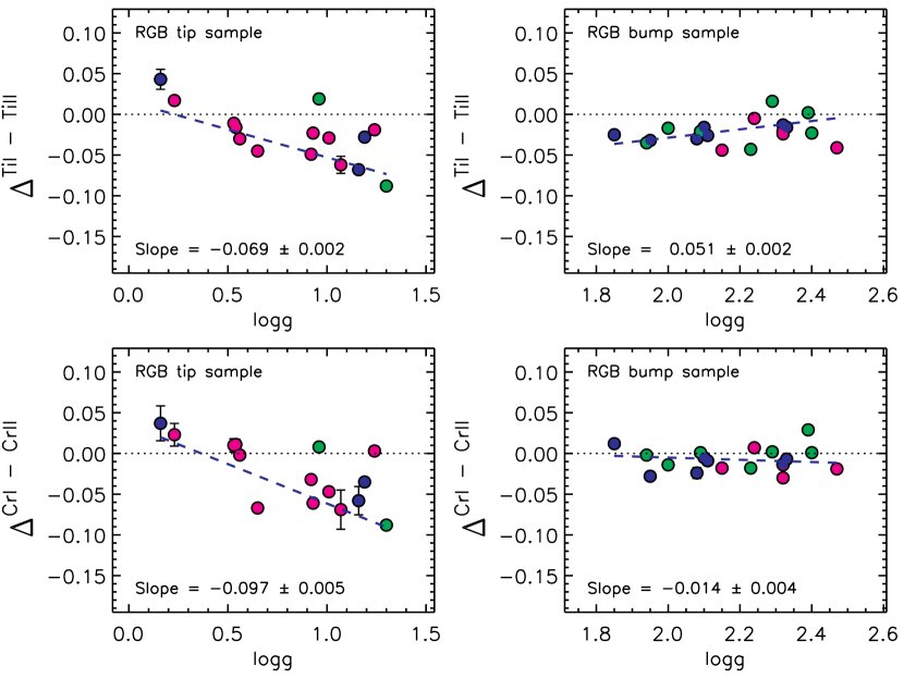
Figure 6: $\Delta^{\rm TiI-TiII}$ (upper panels) and $\Delta^{\rm CrI-CrII}$ (lower panels) for the RGB tip star sample (left panels) and the RGB bump star sample (right panels). (These results are obtained when using the reference stars RGB tip = NGC 6752-mg9 and RGB bump = NGC 6752-11.) The colours are the same as in Figure 4.

2.6 Error Analysis

To determine the errors in the stellar parameters, we adopted the following approach. For $T_{\rm eff}$, we determined the formal uncertainty in the slope between $\delta A_{i}^{\rm FeI}$ and the lower excitation potential. We then adjusted $T_{\rm eff}$ until the formal slope matched the error. The difference between the new $T_{\rm eff}$ and the original value is $\sigma$$T_{\rm eff}$. For the RGB tip and RGB bump stars, the average values of $\sigma$$T_{\rm eff}$ were 7.53 K and 21.74 K, respectively. For $\log g$, we added the standard error of the mean for $\Delta^{\rm FeI}$ and $\Delta^{\rm FeII}$ in quadrature and then adjusted $\log g$ until the quantity $\Delta^{\rm FeI-FeII}$, from equation (5) above, was equal to this value. The difference between the new $\log g$ and the original value is $\sigma$$\log g$. For the RGB tip and RGB bump stars, the average values of $\sigma$$\log g$ were 0.015 dex and 0.009 dex, respectively. For $\xi_{t}$, we measured the formal uncertainty in the slope between $\delta A_{i}^{\rm FeI}$ and the reduced equivalent width. We adjusted $\xi_{t}$ until the formal slope was equal to this value. The difference between the new and old values is $\sigma$$\xi_{t}$. Average values for $\sigma$$\xi_{t}$ for the RGB tip and RGB bump samples were 0.031 km s^-1 and 0.018 km s^-1, respectively.

Uncertainties in the element abundance measurements were obtained following the formalism given in Johnson (2002), which we repeat here for convenience, and we note that this approach is very similar to that of McWilliam et al. (1995) and Barklem et al. (2005).

$$\sigma^{2}_{\rm{log}\epsilon}=\sigma^{2}_{\rm rand}+\left({\partial\rm{log}\epsilon\over\partial T}\right)^{2}\sigma^{2}_{T}+\left({\partial\rm{log}\epsilon\over\partial\rm logg}\right)^{2}\sigma^{2}_{\rm logg}+$$

$$\left({\partial\rm{log}\epsilon\over\partial\xi}\right)^{2}\sigma^{2}_{\xi}+2\biggl{[}\left({\partial\rm{log}\epsilon\over\partial T}\right)\left({\partial\rm{log}\epsilon\over\partial\rm logg}\right)\sigma_{T\rm logg}+$$

$$\left({\partial\rm{log}\epsilon\over\partial\xi}\right)\left({\partial\rm{log}\epsilon\over\partial\rm logg}\right)\sigma_{\rm logg\xi}+\left({\partial\rm{log}\epsilon\over\partial\xi}\right)\left({\partial\rm{log}\epsilon\over T}\right)\sigma_{\xi T}\biggr{]}$$ (6)

The covariance terms, $\sigma_{T\rm logg}$, $\sigma_{\rm logg\xi}$ and $\sigma_{\xi T}$, were computed using the approach of Johnson (2002). These abundance uncertainties are included in Tables 5, 6, 8 and 9. For La and Eu, the abundances were obtained from a single line. For these lines, we adopt the 1$\sigma$ fitting error from the $\chi^{2}$ analysis in place of the random error term, $\sigma_{\rm rand}$ (standard error of the mean). We note that these formal uncertainties, which take into account all covariance error terms, are below 0.02 dex for many elements in many stars, reaching values as low as $\sim$0.01 dex for a number of elements including Si, Ti i, Ni and Fe.

Note that in Figure 6, we regard $\Delta^{\rm TiI-TiII}$ as an abundance ratio between Ti i and Ti ii, and thus, we compute the error terms according to the relevant equations in Johnson (2002) which we again repeat here for convenience.

$$\sigma^{2}(A/B)=\sigma^{2}(A)+\sigma^{2}(B)-2\sigma_{A,B}$$ (7)

The covariance between two abundances is given by

$$\sigma_{A,B}=\left({\partial\rm{log}\epsilon_{A}\over\partial T}\right)\left({\partial\rm{log}\epsilon_{B}\over\partial T}\right)\sigma^{2}_{T}+\hskip 57.81621pt$$

$$\left({\partial\rm{log}\epsilon_{A}\over\partial\rm logg}\right)\left({\partial\rm{log}\epsilon_{B}\over\partial\rm logg}\right)\sigma^{2}_{\rm logg}+\left({\partial\rm{log}\epsilon_{A}\over\partial\xi}\right)\left({\partial\rm{log}\epsilon_{B}\over\partial\xi}\right)\sigma^{2}_{\xi}$$

$$+\biggl{[}\left({\partial\rm{log}\epsilon_{A}\over\partial T}\right)\left({\partial\rm{log}\epsilon_{B}\over\partial\rm logg}\right)+\left({\partial\rm{log}\epsilon_{A}\over\partial\rm logg}\right)\left({\partial\rm{log}\epsilon_{B}\over\partial T}\right)\biggr{]}\sigma_{T\rm logg}$$

$$+\biggl{[}\left({\partial\rm{log}\epsilon_{A}\over\partial\xi}\right)\left({\partial\rm{log}\epsilon_{B}\over\partial\rm logg}\right)+\left({\partial\rm{log}\epsilon_{A}\over\partial\rm logg}\right)\left({\partial\rm{log}\epsilon_{B}\over\partial\xi}\right)\biggr{]}\sigma_{\xi\rm logg}$$ (8)

3 RESULTS AND DISCUSSION

3.1 Trends vs. $T_{\rm eff}$

In Figures 7, 8 and 9, we plot $\Delta^{\rm Fe}$, $\Delta^{\rm CrII}$ and $\Delta^{\rm Ni}$ versus $T_{\rm eff}$, respectively. In these figures, the RGB tip sample and the RGB bump sample are in the upper and lower panels, respectively. In each panel, we show the mean and the abundance dispersion for $\Delta^{\rm X}$ ($\sigma_{\rm A}$ in these figures). We also determine the linear least squares fit to the data and write the slope, uncertainty and abundance dispersion about the fit ($\sigma_{\rm B}$ in these figures). For the subset of RGB tip stars within 100 K and 200 K of the reference star, we compute and write the mean abundance and abundance dispersions ($\sigma_{\rm A}$ and $\sigma_{\rm B}$). Similarly, for the subset of RGB bump stars within 50 K and 100 K of the reference star, we write the same quantities. Finally, we also write the average abundance error, $<\sigma\Delta^{\rm X}>$, for a particular element for the RGB tip and RGB bump samples.

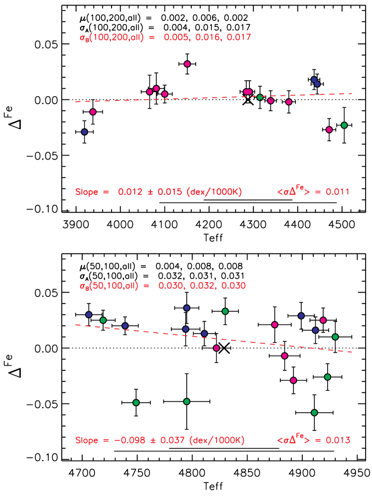
Figure 7: $\Delta^{\rm Fe}$ vs. $T_{\rm eff}$ for the RGB tip star sample (upper panel) and the RGB bump star sample (lower panel). In both panels, we show the location of the “reference star” as a black cross. We write the mean abundance and standard deviation ($\sigma_{\rm A}$) for stars within 100K and 200K of the reference star as well as for the full sample. The red dashed line is the linear least squares fit to the data. The slope, uncertainty and dispersion ($\sigma_{\rm B}$) about the linear fit are written. We also write the average abundance error, $<\sigma\Delta^{\rm Fe}>$, for each sample. (These results are obtained when using the reference stars RGB tip = NGC 6752-mg9 and RGB bump = NGC 6752-11.) The colours are the same as in Figure 4

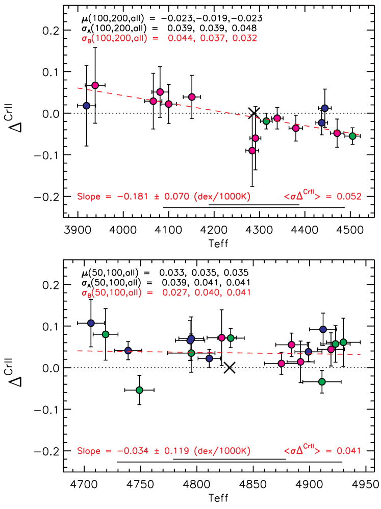
Figure 8: Same as Figure 7 but for $\Delta^{\rm CrII}$ vs. $T_{\rm eff}$.

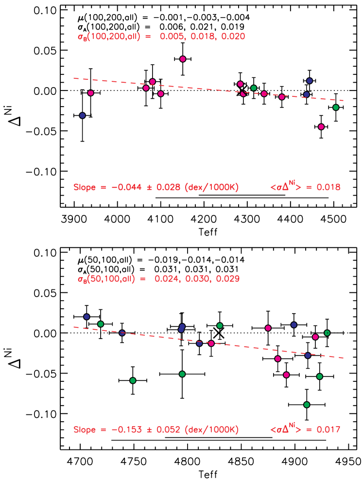
Figure 9: Same as Figure 7 but for $\Delta^{\rm Ni}$ vs. $T_{\rm eff}$.

Fe and Ni (Figures 7 and 9) are examples where the average abundance errors are very small, $\sim$0.01 dex. Cr ii (Figure 8) is the element that shows the highest average abundance error, $\sim$0.04 dex. Rather than showing similar figures for every element, in Figure 10 we plot ($i$) the average abundance error ($<\sigma\Delta^{\rm X}>$), ($ii$) the abundance dispersion ($\sigma_{\rm A}$) and ($iii$) the abundance dispersion about the linear fit to $\Delta^{\rm X}$ versus $T_{\rm eff}$ ($\sigma_{\rm B}$), for all elements in the RGB tip sample (upper) and the RGB bump sample (lower). The main point to take from this figure is that we have achieved very high precision chemical abundance measurements from our strictly differential analysis for this sample of giant stars in the globular cluster NGC 6752. For the RGB tip sample, the lowest average abundance error is for Fe ($<\sigma\Delta^{\rm Fe}>$ = 0.011 dex) and the highest value is for CrII ($<\sigma\Delta^{\rm CrII}>$ = 0.052 dex). For the RGB bump sample the lowest average abundance errors are for Fe and La ($<\sigma\Delta^{\rm Fe,La}>$ = 0.013 dex) while the highest value is for CrII ($<\sigma\Delta^{\rm CrII}>$ = 0.041 dex). Another aspect to note in Figure 10 is that the measured dispersions ($\sigma_{\rm A}$ and $\sigma_{\rm B}$) for many elements appear to be considerably larger than the average abundance error. We interpret such a result as evidence for a genuine abundance dispersion in this cluster, although another possible explanation is that we have systematically underestimated the errors.

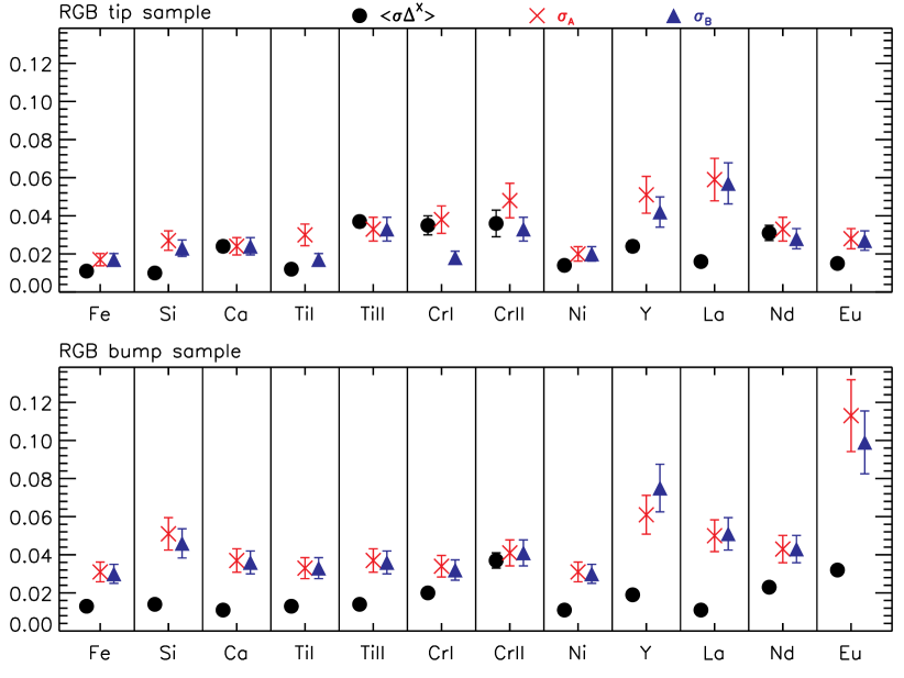
Figure 10: Average abundance errors ($<\sigma\Delta^{X}>$, filled black circles), abundance dispersions ($\sigma_{\rm A}$, red crosses) and abundance dispersions about the linear fits as seen in Figures 7 to 9 ($\sigma_{\rm B}$, blue triangles) for all species in the RGB tip sample (upper panel) and RGB bump sample (lower panel). (These results are obtained when using the reference stars RGB tip = NGC 6752-mg9 and RGB bump = NGC 6752-11.)

3.2 $\Delta^{\rm X}$ vs. $\Delta^{\rm Na}$

In Figures 11 and 12, we plot $\Delta^{\rm Fe}$ vs. $\Delta^{\rm Na}$ and $\Delta^{\rm Si}$ vs. $\Delta^{\rm Na}$, respectively. In both figures, the RGB tip sample and the RGB bump sample are found in the upper and lower panels, respectively. (Here one readily sees that the populations $a$ (green), $b$ (magenta) and $c$ (blue) identified by Milone et al. (2013) from colour-magnitude diagrams have distinct Na abundances.) We measure the linear least squares fit to the data and in each panel we write ($i$) the slope and uncertainty, ($ii$) the abundance dispersion ($\sigma_{\rm A}$), ($iii$) the abundance dispersion about the linear fit to $\Delta^{\rm X}$ versus $\Delta^{\rm Na}$ ($\sigma_{\rm B}$) and (iv) the average abundance error ($<\sigma\Delta^{\rm X}>$). Consideration of the slope and uncertainty of the linear fits reveals that while the amplitude may be small, there are statistically significant correlations between $\Delta^{\rm Fe}$ and $\Delta^{\rm Na}$ for the RGB bump sample and between $\Delta^{\rm Si}$ and $\Delta^{\rm Na}$ for the RGB tip and RGB bump samples. The results for Si confirm and expand on the correlations found between Si and Al (Yong et al., 2005) and between Si and N (Yong et al., 2008).

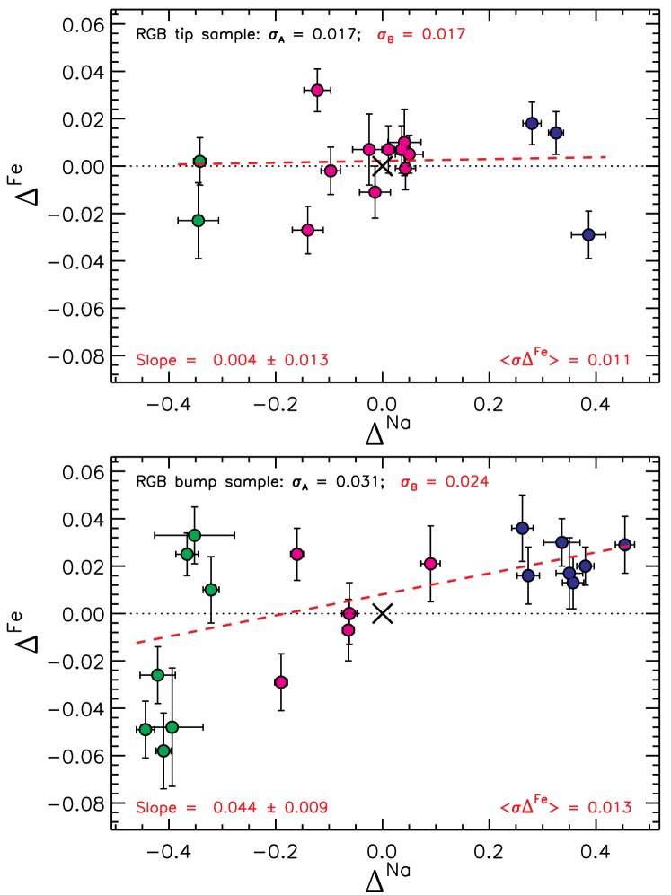
Figure 11: $\Delta^{\rm Fe}$ vs. $\Delta^{\rm Na}$ for the RGB tip star sample (upper) and the RGB bump star sample (lower). The red dashed line is the linear least squares fit to the data (slope and error are written). We write the dispersion in the $y$-direction ($\sigma_{\rm A}$), the dispersion about the linear fit ($\sigma_{\rm B}$) and the average abundance error, $<\sigma\Delta^{\rm Fe}>$, for each sample. (These results are obtained when using the reference stars RGB tip = NGC 6752-mg9 and RGB bump = NGC 6752-11.) The colours are the same as in Figure 4.

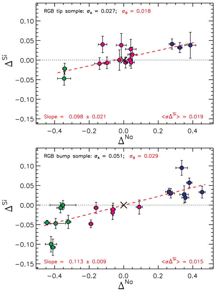
Figure 12: Same as Figure 11 but for $\Delta^{\rm Si}$ vs. $\Delta^{\rm Na}$.

In Figure 13, we plot the slope of the linear fit to $\Delta^{\rm X}$ vs. $\Delta^{\rm Na}$ for all elements in the RGB tip sample (upper) and the RGB bump sample (lower). With the exception of La and Eu (for the RGB tip sample), all the gradients are positive. For La and Eu in the RGB tip sample, the negative gradients are not statistically significant, $<$1$\sigma$. Assuming an equal likelihood of obtaining a positive or negative gradient, the probability of obtaining 22 positive values in a sample of 24 is $\sim$10^-5. Based on the slope and uncertainty, we obtain the significance of the correlations; eight of the 24 elements exhibit correlations that are significant at the 5$\sigma$ level or higher. Therefore, the first main conclusion we draw is that there are an unusually large number of elements that show positive correlations for $\Delta^{\rm X}$ vs. $\Delta^{\rm Na}$, and that an unusually large fraction of these correlations are of high statistical significance. We interpret this result as further evidence for a genuine abundance dispersion in this cluster. On this occasion, it is highly unlikely that such correlations could arise from underestimating the errors. NLTE corrections for Na, using improved atomic data, have been published by Lind et al. (2011a). The corrections are negative and strongly dependent on line strength; for a given $T_{\rm eff}$:$\log g$:[Fe/H], stronger lines have larger amplitude (negative) NLTE corrections. Had we included these corrections, the $\Delta^{\rm X}$ vs. $\Delta^{\rm Na~{}(NLTE)}$ gradients would be even steeper.

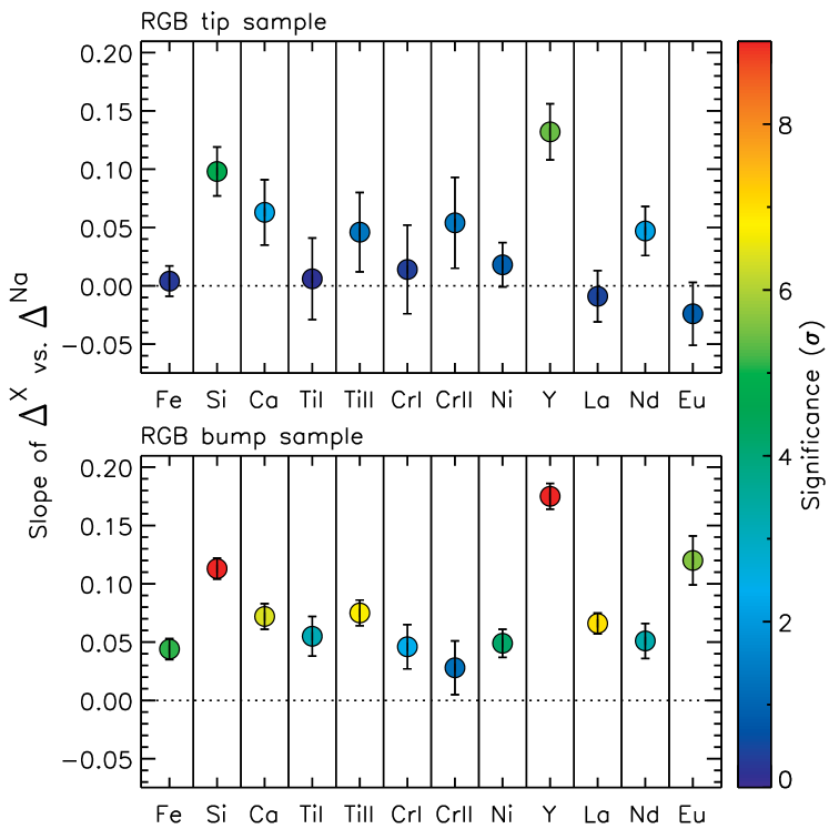
Figure 13: Slope of the fit to $\Delta^{\rm X}$ vs. $\Delta^{\rm Na}$, for X = Si to Eu, for the RGB tip sample (upper) and the RGB bump sample (lower). The colours represent the significance of the slope, i.e., the magnitude of the gradient divided by the uncertainty. (These results are obtained when using the reference stars RGB tip = NGC 6752-mg9 and RGB bump = NGC 6752-11.)

We also note that the gradients are, on average, of larger amplitude and of higher statistical significance for the RGB bump sample compared to the RGB tip sample. Other than spanning a different range in stellar parameters, one notable difference between the two samples is that the RGB bump sample exhibits a larger range in $\Delta^{\rm Na}$ than does the RGB tip sample. In particular, the numbers of RGB tip and RGB bump stars with $|\Delta^{\rm Na}|$ $\geq$ 0.20 dex are five and 14, respectively. (Equivalently, the numbers of stars in the Milone et al. (2013) $b$ and $c$ populations are considerably larger in the RGB bump sample compared to the RGB tip sample.) Thus, we speculate that the RGB bump stars are the more reliable sample (based on the sample size and abundance distribution) from which to infer the presence of any trend between $\Delta^{\rm X}$ vs. $\Delta^{\rm Na}$.

We conducted the following test in order to check whether differences in gradients for $\Delta^{\rm X}$ vs. $\Delta^{\rm Na}$ between the RGB tip and RGB bump samples can be attributed to differences in the Na distributions between the two samples. We start by assuming that the RGB bump sample provides the “correct” slope. For a given element, we consider the gradient and uncertainty for $\Delta^{\rm X}$ vs. $\Delta^{\rm Na}$ and draw a random number from a normal distribution (centered at zero) whose width corresponds to the uncertainty. We add that random number to the gradient to obtain a “new RGB bump gradient” for $\Delta^{\rm X}$ vs. $\Delta^{\rm Na}$. For each RGB tip star, we infer the corresponding $\Delta^{\rm X}$ using this “new RGB bump gradient”. We then draw another random number from a normal distribution (centered at zero) of width corresponding to the measurement uncertainty, $\sigma\Delta^{\rm X}$, and add that number to the $\Delta^{\rm X}$ value inferred. For a given element, we measure the gradient and uncertainty for this new set of $\Delta^{\rm X}$ values. We repeated the process for 1,000,000 realisations. Our expectation is that these Monte Carlo simulations predict the gradient for $\Delta^{\rm X}$ vs. $\Delta^{\rm Na}$ that would be obtained when combining ($i$) the RGB bump sample gradient with ($ii$) the RGB tip sample Na distribution, and this approach accounts for the uncertainties in the RGB bump sample gradients and measurement errors appropriate for the RGB tip sample. For all elements except Fe (61123) and Eu (543), the gradients measured from the RGB tip sample are consistent with those from the simulations. We thus conclude that for most, but not all, elements the differences in the $\Delta^{\rm X}$ vs. $\Delta^{\rm Na}$ gradients for the two samples can be attributed to the differences in the Na distribution.

3.3 $\Delta^{\rm X}$ vs. $\Delta^{\rm Y}$

We now consider $\Delta^{\rm X}$ vs. $\Delta^{\rm Y}$, for every possible combination of elements. In Figures 14 and 15 we plot $\Delta^{\rm Ca}$ vs. $\Delta^{\rm Si}$ and $\Delta^{\rm Nd}$ vs. $\Delta^{\rm Ni}$, respectively. Once again we plot the linear least squares fit to the data and write the slope and uncertainty. Consideration of those quantities reveals that these pairs of elements show a statistically significant correlation, although the amplitudes of the abundance variations are small. In these figures, we write the abundance dispersions and average abundance errors in the $x$-direction and the $y$-direction. As seen in Figure 10, the abundance dispersions are almost always equal to, and in some cases substantially larger than, the average measurement uncertainty.

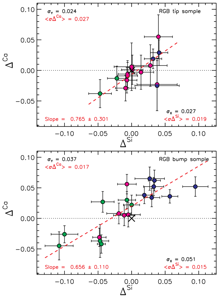
Figure 14: $\Delta^{\rm Ca}$ vs. $\Delta^{\rm Si}$ for the RGB tip sample (upper) and the RGB bump sample (lower). The red dashed line is the linear least squares fit to the data (slope and error are written). We write the abundance dispersions in the $x-$direction ($\sigma_{\rm X}$) and $y$-direction ($\sigma_{\rm Y}$) and the average abundance errors, $<\sigma\Delta^{\rm Ca,Si}>$. (These results are obtained when using the reference stars RGB tip = NGC 6752-mg9 and RGB bump = NGC 6752-11.) The colours are the same as in Figure 4.

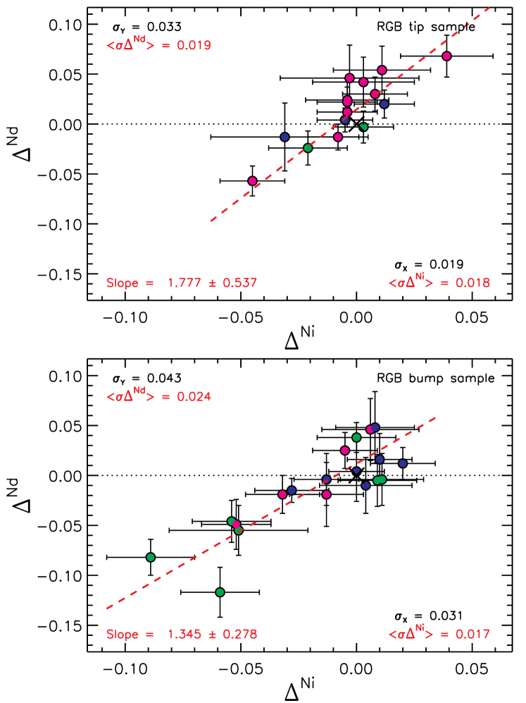
Figure 15: Same as Figure 14 but for $\Delta^{\rm Nd}$ vs. $\Delta^{\rm Ni}$.

In Figure 16, we show the linear fit to $\Delta^{\rm X}$ vs. $\Delta^{\rm Y}$ for all combinations of elements for the RGB tip sample. The significance for a pair of elements, which is based on the slope and the uncertainty, is shown in this figure. The gradients are always positive, with the exception of the following pair of elements, Si and Eu (consideration of the uncertainty suggests that the gradients are not significant). That is, 65 out of 66 pairs of elements exhibit a positive correlation. The average gradient is 2.14 $\pm$ 0.29 ($\sigma$ = 2.37).

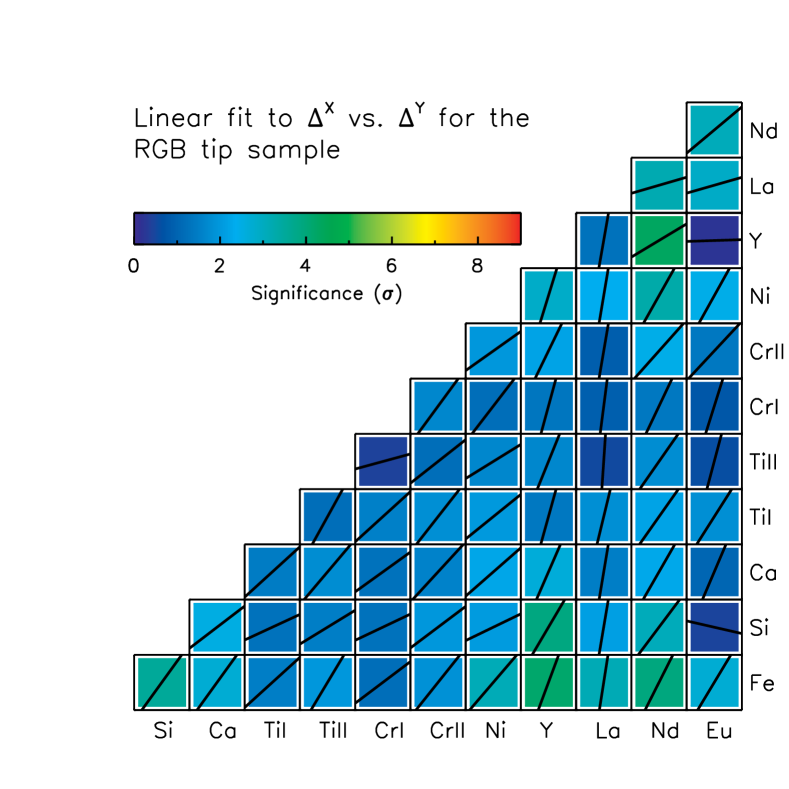
Figure 16: Linear fit to $\Delta^{\rm X}$ vs. $\Delta^{\rm Y}$, for all combination of elements, for the RGB tip sample. The dimensions of the x-axis and y-axis are unity, such that a slope of gradient 1.0 would be represented by a straight line from the lower left corner to the upper right corner and a slope of gradient 0.0 would be a horizontal line. The significance of the gradients are indicated by the colour bar. (These results are obtained when using the reference stars RGB tip = NGC 6752-mg9 and RGB bump = NGC 6752-11.)

Figure 17 is the same as Figure 16, but for the RGB bump sample. The gradients are always positive with an average value of 2.52 $\pm$ 0.40 ($\sigma$ = 3.29). Interestingly, the gradients are, in general, of considerably higher statistical significance than in the RGB tip sample. The average significance of the correlations is 2.0$\sigma$ for the RGB tip sample and 4.5$\sigma$ for the RGB bump sample. For the RGB bump sample, 25 pairs of elements (out of a total of 66) exhibit correlations that are significant at the 5$\sigma$ level or higher. Thus, the second main conclusion we draw is that there are an unusually large number of elements that show positive correlations for $\Delta^{\rm X}$ vs. $\Delta^{\rm Y}$ and that many of these pairs of elements exhibit correlations that are of high statistical significance. Again, we speculate that the higher statistical significance for the correlations between pairs of elements in the RGB bump sample, compared to the RGB tip sample, is due to the sample size and abundance distribution (i.e., the RGB bump sample includes many more stars at the extremes of the $\Delta^{\rm Na}$, and therefore $\Delta^{\rm X}$, distributions). Monte Carlo simulations indicate that the gradients for the RGB bump and RGB tip samples are consistent when taking into account the different distributions in $\Delta^{\rm X}$ between the two samples. We interpret the significant correlations bewteen $\Delta^{\rm X}$ and $\Delta^{\rm Y}$ as further indication of a genuine abundance dispersion in this globular cluster.

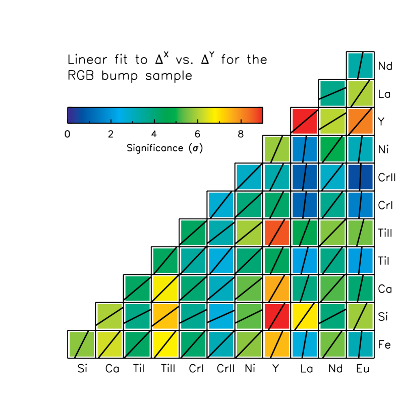
Figure 17: Same as Figure 16 but for the RGB bump sample.

3.4 Removing Trends With $T_{\rm eff}$

Inspection of Figures 7, 8 and 9 suggests that there are statistically significant trends between $\Delta^{\rm X}$ and $T_{\rm eff}$. We tentatively attribute those abundance trends with $T_{\rm eff}$ to differential non-LTE effects and/or 3D effects (e.g., Asplund 2005). In this subsection, we explore whether or not our results change if we remove the abundance trends with $T_{\rm eff}$. That is, do the abundance trends between ($i$) $\Delta^{\rm X}$ vs. $\Delta^{\rm Na}$ and ($ii$) $\Delta^{\rm X}$ vs. $\Delta^{\rm Y}$ persist, or disappear, if we remove the abundance trends with $T_{\rm eff}$?

We remove those abundance trends with $T_{\rm eff}$ in the following manner. We define a new quantity, $\Delta^{\rm X}_{\rm T}$, as the difference between $\Delta^{\rm X}$ and the value of the linear fit to the data at the $T_{\rm eff}$ of the program star. In Figure 18, we plot the slope of $\Delta^{\rm X}_{\rm T}$ vs. $\Delta^{\rm Na}_{\rm T}$. This figure is similar to Figure 13, but we have removed the abundance trends with $T_{\rm eff}$. With the exception of Y in the RGB bump sample, our results are unchanged at the $<$1.0$\sigma$ level. For Y, the slope and error changed from 0.174 $\pm$ 0.011 to 0.131 $\pm$ 0.010, a difference of 3$\sigma$; in both cases the correlation is of high statistical significance.

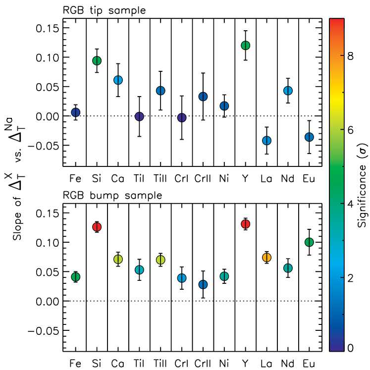
Figure 18: Same as Figure 13 but for $\Delta^{\rm X}_{\rm T}$ vs. $\Delta^{\rm Na}_{\rm T}$, i.e., the abundance trends with $T_{\rm eff}$ have been removed as described in Section 3.4. (These results are obtained when using the reference stars RGB tip = NGC 6752-mg9 and RGB bump = NGC 6752-11.)

Next, we examine the trends between $\Delta^{\rm X}_{\rm T}$ vs. $\Delta^{\rm Y}_{\rm T}$ (see Figures 19 and 20). These figures are the same as Figures 16 and 17 but we have removed the abundance trends with $T_{\rm eff}$. On comparing the RGB tip samples (Figures 16 vs. 19) and the RGB bump samples (Figures 17 vs. 20), the results are unchanged, at the $<$2$\sigma$ level, for all pairs of elements. Therefore, we find positive correlations of high statistical significance between pairs of elements regardless of whether or not we remove any abundance trends with $T_{\rm eff}$. Such a result increases our confidence that the abundance trends we identify are real and not an artefact of systematic errors in the analysis.

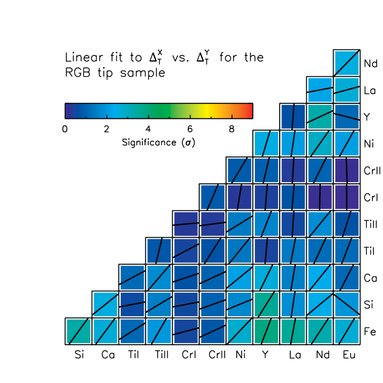
Figure 19: Same as Figure 16 but for $\Delta^{\rm X}_{\rm T}$ vs. $\Delta^{\rm Y}_{\rm T}$ in the RGB tip sample, i.e., the abundance trends with $T_{\rm eff}$ have been removed as described in Section 3.4. (These results are obtained when using the reference stars RGB tip = NGC 6752-mg9 and RGB bump = NGC 6752-11.)

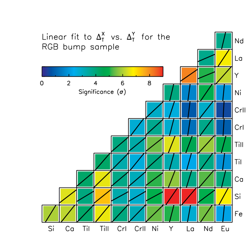
Figure 20: Same as Figure 19 but for the RGB bump sample.

3.5 Confirmation of Results When Using a Different Reference Star

An important consideration is whether or not the results change for a different choice of reference stars. In this subsection, we repeat the entire analysis but using a new pair of reference stars. For the RGB tip sample and RGB bump sample, we use NGC 6752-mg6 and NGC 6752-1 as the reference stars, respectively. These stars were arbitrarily chosen to have higher S/N (and therefore lower $T_{\rm eff}$) than the previous pair of reference stars.

Starting with the reference star parameters as described in Section 2.3, we obtained for each star in each sample, strictly differential stellar parameters using the line-by-line analysis described in Section 2.4. The new strictly differential stellar parameters are presented in Table 7. As before, the strictly differential stellar parameters are very close to the “reference star” stellar parameters.

Table 7: Strictly Differential Stellar Parameters, and Uncertainties, When Adopting the Second Set of Reference Stars (RGB Tip = NGC 6752-mg6, RGB Bump = NGC 6752-1).

Name	$T_{\rm eff}$	$\sigma$	$\log g$	$\sigma$	$\xi_{t}$	$\sigma$	[Fe/H]
	(K)	(K)	(cm s-2)	(cm s-2)	(km s-1)	(km s-1)
(1)	(2)	(3)	(4)	(5)	(6)	(7)	(8)
NGC6752-mg0	3922	20	0.19	0.01	2.24	0.04	$-$1.68
NGC6752-mg2	3940	16	0.25	0.01	2.11	0.04	$-$1.66
NGC6752-mg3	4070	14	0.55	0.01	1.92	0.03	$-$1.64
NGC6752-mg4	4087	14	0.57	0.01	1.90	0.03	$-$1.64
NGC6752-mg5	4105	16	0.59	0.01	1.93	0.04	$-$1.64
NGC6752-mg8	4288	17	0.98	0.01	1.71	0.04	$-$1.64
NGC6752-mg9	4292	20	0.96	0.01	1.73	0.05	$-$1.65
NGC6752-mg10	4295	14	0.96	0.01	1.69	0.04	$-$1.64
NGC6752-mg12	4315	17	1.00	0.01	1.73	0.05	$-$1.65
NGC6752-mg15	4347	17	1.04	0.01	1.77	0.05	$-$1.65
NGC6752-mg18	4387	13	1.10	0.01	1.70	0.04	$-$1.65
NGC6752-mg21	4443	16	1.19	0.01	1.69	0.06	$-$1.63
NGC6752-mg22	4451	18	1.23	0.01	1.71	0.07	$-$1.64
NGC6752-mg24	4511	16	1.33	0.01	1.70	0.06	$-$1.67
NGC6752-mg25	4479	15	1.28	0.01	1.72	0.06	$-$1.67
NGC6752-0	4737	11	1.86	0.01	1.44	0.02	$-$1.62
NGC6752-2	4770	10	1.95	0.01	1.36	0.02	$-$1.63
NGC6752-3	4781	11	1.98	0.01	1.36	0.02	$-$1.70
NGC6752-4	4827	12	2.07	0.01	1.39	0.02	$-$1.63
NGC6752-6	4830	13	2.10	0.01	1.34	0.02	$-$1.61
NGC6752-8	4966	16	2.29	0.01	1.33	0.03	$-$1.64
NGC6752-9	4829	18	2.08	0.01	1.42	0.03	$-$1.69
NGC6752-10	4846	12	2.10	0.01	1.38	0.02	$-$1.63
NGC6752-11	4866	6	2.13	0.01	1.37	0.02	$-$1.64
NGC6752-12	4855	13	2.14	0.01	1.35	0.02	$-$1.64
NGC6752-15	4866	15	2.23	0.01	1.37	0.02	$-$1.61
NGC6752-16	4911	15	2.24	0.01	1.33	0.03	$-$1.62
NGC6752-19	4928	12	2.32	0.01	1.33	0.02	$-$1.67
NGC6752-20	4935	13	2.33	0.01	1.32	0.02	$-$1.62
NGC6752-21	4921	14	2.32	0.01	1.32	0.03	$-$1.65
NGC6752-23	4945	12	2.32	0.01	1.26	0.02	$-$1.63
NGC6752-24	4945	14	2.39	0.01	1.15	0.03	$-$1.70
NGC6752-29	4959	12	2.40	0.01	1.32	0.02	$-$1.67
NGC6752-30	4954	13	2.47	0.01	1.25	0.02	$-$1.62

With these revised stellar parameters, we computed chemical abundances and conducted a full error analysis following the procedures outlined in Sections 2.5 and 2.6, respectively. In Tables 8 and 9 we present the abundance differences for each element in all program stars when using this new pair of reference stars. (We did not, however, recompute abundances based on spectrum synthesis analysis for La and Eu, and thus those elements will not be considered in this subsection). Again, we achieve high precision chemical abundance measurements and the measured dispersions ($\sigma_{\rm A}$, $\sigma_{\rm B}$) are, in general, larger than the average abundance error (particularly for the RGB bump sample).

Table 8: Differential Abundances (Fe, Na, Si, Ca and Ti) When Adopting the Second Set of Reference Stars (RGB Tip = NGC 6752-mg6, RGB Bump = NGC 6752-1).

Star	$\Delta^{\rm Fe}$	$\sigma$	$\Delta^{\rm Na}$	$\sigma$	$\Delta^{\rm Si}$	$\sigma$	$\Delta^{\rm Ca}$	$\sigma$	$\Delta^{\rm TiI}$	$\sigma$	$\Delta^{\rm TiII}$	$\sigma$
(1)	(2)	(3)	(4)	(5)	(6)	(7)	(8)	(9)	(10)	(11)	(12)	(13)
NGC6752-mg0	$-$0.065	0.009	0.387	0.030	0.043	0.032	$-$0.022	0.040	0.023	0.050	$-$0.013	0.049
NGC6752-mg2	$-$0.047	0.011	$-$0.014	0.017	0.044	0.019	$-$0.017	0.028	0.054	0.035	0.050	0.038
NGC6752-mg3	$-$0.027	0.014	$-$0.026	0.026	0.012	0.025	0.001	0.031	0.024	0.044	0.056	0.046
NGC6752-mg4	$-$0.024	0.010	0.043	0.024	0.037	0.020	0.012	0.025	0.029	0.034	0.058	0.037
NGC6752-mg5	$-$0.029	0.008	0.052	0.021	0.023	0.020	0.002	0.030	0.010	0.039	0.054	0.046
NGC6752-mg8	$-$0.036	0.016	0.038	0.002	0.007	0.006	0.008	0.011	0.015	0.010	0.052	0.066
NGC6752-mg9	$-$0.036	0.016	0.002	0.018	0.006	0.019	$-$0.001	0.025	0.005	0.027	0.013	0.023
NGC6752-mg10	$-$0.028	0.011	0.015	0.014	0.003	0.016	$-$0.002	0.022	$-$0.018	0.024	0.043	0.017
NGC6752-mg12	$-$0.038	0.013	$-$0.347	0.024	$-$0.020	0.017	$-$0.020	0.028	0.004	0.043	0.004	0.026
NGC6752-mg15	$-$0.036	0.013	0.048	0.024	$-$0.002	0.018	$-$0.005	0.031	$-$0.002	0.040	0.022	0.033
NGC6752-mg18	$-$0.036	0.009	$-$0.093	0.017	$-$0.000	0.014	$-$0.011	0.020	$-$0.012	0.027	0.061	0.032
NGC6752-mg21	$-$0.018	0.011	0.283	0.019	0.048	0.015	0.034	0.025	$-$0.007	0.031	0.072	0.033
NGC6752-mg22	$-$0.021	0.013	0.326	0.015	0.035	0.016	0.020	0.022	$-$0.005	0.033	0.025	0.033
NGC6752-mg24	$-$0.056	0.015	$-$0.341	0.038	$-$0.043	0.016	$-$0.033	0.023	$-$0.026	0.027	0.066	0.063
NGC6752-mg25	$-$0.059	0.009	$-$0.135	0.026	$-$0.002	0.014	$-$0.022	0.019	$-$0.037	0.024	$-$0.001	0.038
NGC6752-0	0.006	0.009	0.699	0.051	0.105	0.024	0.021	0.014	0.020	0.021	0.019	0.016
NGC6752-2	$-$0.004	0.012	0.750	0.016	0.065	0.020	0.010	0.016	$-$0.005	0.020	$-$0.000	0.012
NGC6752-3	$-$0.071	0.012	$-$0.075	0.010	$-$0.032	0.018	$-$0.069	0.015	$-$0.054	0.020	$-$0.070	0.011
NGC6752-4	$-$0.002	0.015	0.726	0.044	0.041	0.015	0.043	0.018	0.008	0.027	0.002	0.012
NGC6752-6	0.019	0.016	0.636	0.014	0.048	0.014	0.039	0.019	0.030	0.027	0.015	0.013
NGC6752-8	$-$0.012	0.015	0.045	0.014	$-$0.032	0.014	$-$0.002	0.015	0.026	0.024	$-$0.019	0.017
NGC6752-9	$-$0.065	0.022	$-$0.024	0.038	$-$0.034	0.017	$-$0.060	0.024	$-$0.061	0.037	$-$0.074	0.012
NGC6752-10	$-$0.006	0.014	0.730	0.014	0.032	0.014	0.015	0.017	0.007	0.025	$-$0.002	0.013
NGC6752-11	$-$0.019	0.006	0.373	0.021	0.016	0.013	$-$0.024	0.011	0.001	0.015	$-$0.030	0.012
NGC6752-12	$-$0.018	0.014	0.306	0.016	0.003	0.017	$-$0.020	0.016	$-$0.022	0.026	$-$0.001	0.016
NGC6752-15	0.013	0.015	0.018	0.056	0.013	0.019	$-$0.003	0.019	$-$0.005	0.027	0.010	0.013
NGC6752-16	0.001	0.014	0.461	0.035	0.009	0.024	$-$0.017	0.017	0.001	0.025	$-$0.023	0.016
NGC6752-19	$-$0.050	0.013	0.179	0.014	$-$0.034	0.022	$-$0.056	0.014	$-$0.048	0.020	$-$0.055	0.013
NGC6752-20	0.009	0.012	0.822	0.036	0.045	0.018	0.024	0.016	0.019	0.023	0.006	0.013
NGC6752-21	$-$0.027	0.013	0.308	0.023	$-$0.005	0.019	$-$0.015	0.017	$-$0.009	0.022	$-$0.021	0.012
NGC6752-23	$-$0.006	0.012	0.641	0.009	0.045	0.018	0.005	0.015	$-$0.006	0.023	$-$0.012	0.017
NGC6752-24	$-$0.079	0.012	$-$0.041	0.013	$-$0.094	0.014	$-$0.076	0.018	$-$0.082	0.022	$-$0.110	0.013
NGC6752-29	$-$0.048	0.012	$-$0.052	0.013	$-$0.088	0.018	$-$0.054	0.014	$-$0.066	0.029	$-$0.077	0.011
NGC6752-30	0.004	0.012	0.207	0.013	0.005	0.013	0.030	0.016	0.001	0.024	0.020	0.015

Table 9: Differential Abundances (Cr, Ni, Y and Nd) When Adopting the Second Set of Reference Stars (RGB Tip = NGC 6752-mg6, RGB Bump = NGC 6752-1).

Star	$\Delta^{\rm CrI}$	$\sigma$	$\Delta^{\rm CrII}$	$\sigma$	$\Delta^{\rm Ni}$	$\sigma$	$\Delta^{\rm Y}$	$\sigma$	$\Delta^{\rm Nd}$	$\sigma$
(1)	(2)	(3)	(4)	(5)	(6)	(7)	(8)	(9)	(10)	(11)
NGC6752-mg0	0.011	0.067	0.028	0.093	$-$0.023	0.030	0.034	0.038	0.003	0.033
NGC6752-mg2	0.053	0.090	0.076	0.077	0.007	0.027	0.101	0.049	0.067	0.030
NGC6752-mg3	0.044	0.055	0.053	0.059	0.013	0.018	0.092	0.025	0.062	0.021
NGC6752-mg4	0.053	0.052	0.068	0.049	0.021	0.018	0.090	0.023	0.075	0.021
NGC6752-mg5	0.034	0.045	0.038	0.049	0.008	0.018	0.025	0.039	0.049	0.020
NGC6752-mg8	$-$0.025	0.044	$-$0.079	0.024	0.018	0.012	0.039	0.031	0.052	0.014
NGC6752-mg9	0.002	0.036	0.014	0.086	0.008	0.017	0.019	0.016	0.020	0.019
NGC6752-mg10	$-$0.006	0.028	$-$0.040	0.076	0.008	0.015	0.100	0.024	0.042	0.016
NGC6752-mg12	$-$0.008	0.032	$-$0.010	0.034	0.006	0.017	0.005	0.017	0.019	0.019
NGC6752-mg15	$-$0.024	0.032	$-$0.006	0.036	0.002	0.017	0.014	0.016	0.032	0.018
NGC6752-mg18	$-$0.022	0.025	$-$0.021	0.030	0.002	0.012	0.032	0.018	0.009	0.012
NGC6752-mg21	$-$0.000	0.031	$-$0.009	0.038	0.005	0.014	0.085	0.021	0.029	0.014
NGC6752-mg22	$-$0.014	0.048	0.019	0.053	0.016	0.016	0.062	0.029	0.030	0.016
NGC6752-mg24	$-$0.028	0.022	$-$0.047	0.019	$-$0.015	0.016	$-$0.045	0.015	$-$0.012	0.016
NGC6752-mg25	$-$0.019	0.027	$-$0.033	0.029	$-$0.033	0.013	$-$0.016	0.026	$-$0.026	0.014
NGC6752-0	0.021	0.021	0.034	0.021	0.012	0.016	0.020	0.012	0.030	0.021
NGC6752-2	$-$0.028	0.025	$-$0.038	0.063	$-$0.012	0.016	$-$0.041	0.044	0.002	0.012
NGC6752-3	$-$0.088	0.023	$-$0.127	0.085	$-$0.064	0.021	$-$0.171	0.030	$-$0.104	0.015
NGC6752-4	$-$0.018	0.029	$-$0.011	0.018	$-$0.001	0.020	$-$0.008	0.045	$-$0.004	0.017
NGC6752-6	0.008	0.039	$-$0.001	0.014	0.002	0.020	$-$0.016	0.031	0.056	0.028
NGC6752-8	$-$0.019	0.029	$-$0.016	0.024	$-$0.008	0.021	$-$0.051	0.011	0.043	0.027
NGC6752-9	$-$0.071	0.040	$-$0.042	0.023	$-$0.056	0.030	$-$0.109	0.017	$-$0.051	0.011
NGC6752-10	$-$0.007	0.029	$-$0.057	0.078	$-$0.019	0.018	$-$0.008	0.022	$-$0.001	0.015
NGC6752-11	$-$0.034	0.015	$-$0.072	0.061	$-$0.002	0.015	$-$0.019	0.028	0.015	0.025
NGC6752-12	$-$0.027	0.030	0.002	0.013	$-$0.020	0.020	$-$0.118	0.036	$-$0.008	0.010
NGC6752-15	$-$0.012	0.033	$-$0.000	0.049	0.002	0.020	$-$0.066	0.009	0.005	0.017
NGC6752-16	$-$0.020	0.026	$-$0.060	0.066	0.004	0.024	$-$0.068	0.031	0.060	0.034
NGC6752-19	$-$0.073	0.026	$-$0.056	0.018	$-$0.055	0.015	$-$0.127	0.028	$-$0.034	0.012
NGC6752-20	$-$0.013	0.028	$-$0.034	0.073	0.003	0.020	$-$0.008	0.019	0.026	0.012
NGC6752-21	$-$0.049	0.024	$-$0.021	0.057	$-$0.035	0.019	$-$0.033	0.014	$-$0.007	0.015
NGC6752-23	$-$0.031	0.033	0.025	0.031	$-$0.033	0.018	$-$0.010	0.029	0.005	0.026
NGC6752-24	$-$0.093	0.023	$-$0.103	0.077	$-$0.095	0.023	$-$0.156	0.015	$-$0.061	0.024
NGC6752-29	$-$0.075	0.024	$-$0.023	0.021	$-$0.061	0.019	$-$0.104	0.007	$-$0.041	0.025
NGC6752-30	$-$0.006	0.026	$-$0.026	0.026	$-$0.012	0.017	$-$0.022	0.043	0.038	0.016

We examine the abundance trends $\Delta^{\rm X}$ versus $\Delta^{\rm Na}$ and $\Delta^{\rm X}_{\rm T}$ versus $\Delta^{\rm Na}_{\rm T}$ in Figures 21 and 22, respectively. As in Sections 3.2 and 3.4, we find that the abundance trends with Na are always positive and that a large number of elements exhibit statistically significant correlations, albeit of small amplitude. These results remain even after removing the abundance trends as a function of $T_{\rm eff}$.

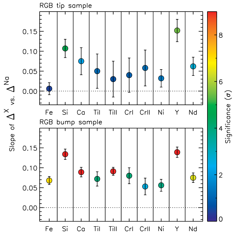
Figure 21: Slope of the fit to $\Delta^{\rm X}$ vs. $\Delta^{\rm Na}$, for X = Si to Eu, for the RGB tip sample (upper) and the RGB bump sample (lower). The colours represent the significance of the slope. (This shows the same results as Figure 13 but for a different pair of reference stars, RGB tip = NGC 6752-mg6 and RGB bump = NGC 6752-1.)

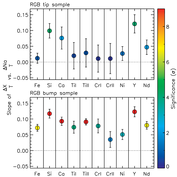
Figure 22: Same as Figure 21 but for $\Delta^{\rm X}_{\rm T}$ vs. $\Delta^{\rm Na}_{\rm T}$, i.e., the abundance trends with $T_{\rm eff}$ have been removed as described in Section 3.4. (These results are obtained when using the reference stars RGB tip = NGC 6752-mg6 and RGB bump = NGC 6752-1.)

Finally, we consider the abundance trends $\Delta^{\rm X}$ versus $\Delta^{\rm Y}$. Our results are essentially identical to those in Sections 3.3 and 3.4, namely, that for many pairs of elements, there are positive correlations of high statistical significance for $\Delta^{\rm X}$ versus $\Delta^{\rm Y}$. Again, these results remain even after removing the abundance trends with $T_{\rm eff}$.

The essential point to take from this subsection is that our results are not sensitive to the choice of reference star, at least for the two cases we investigated.

3.6 Consequences for Globular Cluster Chemical Evolution

We begin with a summary of our analysis and results.

1. From a strictly differential line-by-line analysis of a sample of RGB tip stars and RGB bump stars in the globular cluster NGC 6752, we have obtained revised stellar parameters which we refer to as “strictly differential” stellar parameters.

2. Using those “strictly differential” stellar parameters, we have computed differential chemical abundances, $\Delta^{\rm X}$ (for X = Fe, Na, Si, Ca, Ti, Cr, Ni, Y, La, Nd and Eu), and conducted a detailed error analysis.

3. We have achieved very high precision measurements; for a given element, our average relative abundance errors range from 0.01 dex to 0.05 dex.

4. When plotting our abundance ratios against Na, e.g., $\Delta^{\rm X}$ versus $\Delta^{\rm Na}$, an unusually large number of elements show positive correlations, often of high statistical significance, although the amplitudes of the abundance variations in $\Delta^{\rm X}$ are small.

5. When plotting the abundance ratios for any pair of elements, $\Delta^{\rm X}$ versus $\Delta^{\rm Y}$, the majority exhibit positive correlations, often of high statistical significance.

6. Points (iv) and (v) persist even after ($a$) removing abundance trends with $T_{\rm eff}$ and/or ($b$) conducting a re-analysis using a different pair of reference stars, thereby increasing our confidence in these results.

We now explore the consequences for globular cluster chemical evolution.

At face value, our results would suggest that the globular cluster NGC 6752 is not chemically homogeneous at the $\sim$0.03 dex level for the elements studied here. Chemical inhomogeneity at this level can only be revealed when the measurement uncertainties are $<$0.03 dex, as in this study. By extension, we speculate that other globular clusters with no obvious dispersion in Fe-peak elements but large Na variations (e.g., 47 Tuc, NGC 6397) may also display similar behavior to NGC 6752 if subjected to a strictly differential chemical abundance analysis of comparably high-quality spectra to that of this study.

The abundance variations and positive correlations between $\Delta^{\rm X}$ versus $\Delta^{\rm Na}$ and between $\Delta^{\rm X}$ versus $\Delta^{\rm Y}$ could be due to a number of possibilities. Here we discuss four potential scenarios, which are not mutually exclusive: (1) systematic errors in the stellar parameters; (2) star-to-star CNO abundance variations; (3) star-to-star helium abundance variations; (4) inhomogeneous chemical evolution in the early stages of globular cluster formation.

3.6.1 Systematic errors in the stellar parameters

In the first scenario, we assume that the abundance variations are due to systematic errors in the stellar parameters. As noted in Section 3.1, the abundance dispersions often exceed the average abundance error. Attributing the abundance variations to systematic errors in the stellar parameters would require a substantial underestimate of the stellar parameter uncertainties. Such an explanation may be plausible. However, the abundance variations are highly correlated and are seen for all elements which cover a variety of ionization potentials and ionization states. There is no single change in $T_{\rm eff}$, $\log g$ or $\xi_{t}$ that would remove the abundance correlations for all elements in any given star. Thus, we regard this hypothesis to be unlikely.

3.6.2 Star-to-star CNO abundance variations

In the second scenario, we assume that the abundance variations and correlations are due to neglect of the appropriate C, N and O abundances in the model atmospheres. The structure of the model atmosphere depends upon the adopted C, N and O abundances (Gustafsson et al., 1975). Drake et al. (1993) studied the effect of CNO abundances on the atmospheric structure in giant stars with metallicities similar to that of NGC 6752. For the outer layers of the atmosphere, the “CN-weak” models (i.e., appropriate for Na-poor objects) were cooler than the “CN-strong” models (i.e., appropriate for Na-rich objects) and the maximum difference was $\sim$ 150K. The differences in abundances derived using the “CN-strong” models minus those from the “CN-weak” models for the $T_{\rm eff}$ = 4400K, $\log g$ = 1.3 and [Fe/H] = $-$1.5 case are almost all positive and range from $\sim$ 0.00 dex to $\sim$ 0.10 dex. While the magnitudes of the predicted abundance differences are similar to those of this study, these differences have the incorrect sign. That is, if we had analysed the most Na-rich stars using the “CN-strong” models, according to the Drake et al. (1993) predictions the inferred abundances would be higher and the slope of the correlations between $\Delta^{\rm X}$ and $\Delta^{\rm Na}$ would be even steeper. We note, however, that the vast majority of our lines are weak ($\log(W_{\lambda}/\lambda)$ $\leq$ $-$5.0) such that the predicted abundance differences are essentially zero and thus application of “CN-strong” models with appropriate CNO abundances to the Na-rich stars would not change the trends we find.

In the Drake et al. (1993) models, the C+N+O abundance sum was constant to within 0.12 dex between the “CN-weak” and “CN-strong” models. This assumption of almost constant C+N+O abundance is appropriate for NGC 6752 on two grounds. First, the presence of a substantial C+N+O abundance variation would manifest as a spread in the luminosity of subgiant branch stars (Rood & Crocker, 1985) and such a feature has not been detected in this cluster (Milone et al., 2013). Second, within their measurement uncertainties, Carretta et al. (2005) found no evidence for a dispersion in the C+N+O abundance sum in NGC 6752 and preliminary work we are conducting also indicates a nearly constant C+N+O abundance sum.

3.6.3 Star-to-star helium abundance variations

In the third scenario, we assume that the abundance variations and correlations are due to star-to-star He abundance variations. A detailed analysis of the highest quality colour-magnitude diagrams available shows that NGC 6752 harbours an internal He spread of up to $\Delta Y$ $\sim$ 0.03 (Milone et al., 2013). The most Na-rich objects are assumed to be more He-rich relative to the Na-poor objects. Spectroscopic analysis by Villanova et al. (2009) showed that He measurements are possible in the cooler blue horizontal branch stars of NGC 6752; they found a uniform He content, a result not unexpected given the O-Na abundances of their targets.

He abundance variations would affect our analysis in two distinct ways. First, the structure of the model atmosphere depends upon the adopted He abundance (Strömgren et al., 1982). Second, for a fixed mass fraction of metals ($Z$), a change in the helium mass fraction ($Y$) will directly affect the hydrogen mass fraction ($X$) such that the metal-to-hydrogen ratio, $Z$/$X$ will change with helium mass fraction since $X+Y+Z=1$. We now consider both cases.

Regarding the effect of He on the structure of a model atmosphere, Strömgren et al. (1982) demonstrated that for F type dwarfs, changes in the He/H ratio “affect the mean molecular weight of the gas and have an impact on the gas pressure” and that “a helium-enriched atmosphere is similar to a helium-normal atmosphere with a higher surface gravity, in terms of temperature structure and electron pressure structure” (Lind et al., 2011b). Equation 12 in Strömgren et al. (1982) quantifies the change in $\log g$ due to a change in He/H ratio; Lind et al. (2011b) showed that metal-poor giants behave similarly. From this equation, a change in He abundance from $Y$ = 0.25 to $Y$ = 0.28 would result in a shift in $\log g$ of 0.012. Inclusion of He abundance variations in the model atmospheres would naively be expected to result in different stellar parameters than those derived in this work, for both a regular analysis (as used to define the reference star stellar parameters) and a strictly differential analysis. Using a revised set of stellar parameters would, of course, result in an updated set of chemical abundances (and line-by-line chemical abundance differences).

We might therefore expect to find a correlation between the Na abundance (which is assumed to trace the He abundance) and the stellar parameters (or difference between the strictly differential stellar parameters and the reference star stellar parameters). In Figure 23, we plot $\Delta^{\rm Na}$ against $\Delta$$\log g$ (“reference star” values minus “strictly differential analysis” values). There are no significant correlations for either the RGB tip sample or the RGB bump sample. In light of the statistically significant correlation between Si and Na, we also include in Figure 23 panels showing $\Delta^{\rm Si}$ against $\Delta$$\log g$. Again, there are no significant correlations. (Similar plots using $\Delta$$T_{\rm eff}$ rather than $\Delta$$\log g$ also reveal no significant correlations.) Given the magnitude of the change in $\log g$ resulting from the difference in helium abundance, it is not surprising that we do not detect any significant trend between $\Delta^{\rm Na}$ and $\Delta$$\log g$. Indeed, Lind et al. (2011b) find that changes in helium of $\Delta Y$ = 0.03, as is the case for NGC 6752, would be expected to result in negligible changes in $T_{\rm eff}$ and $\log g$.

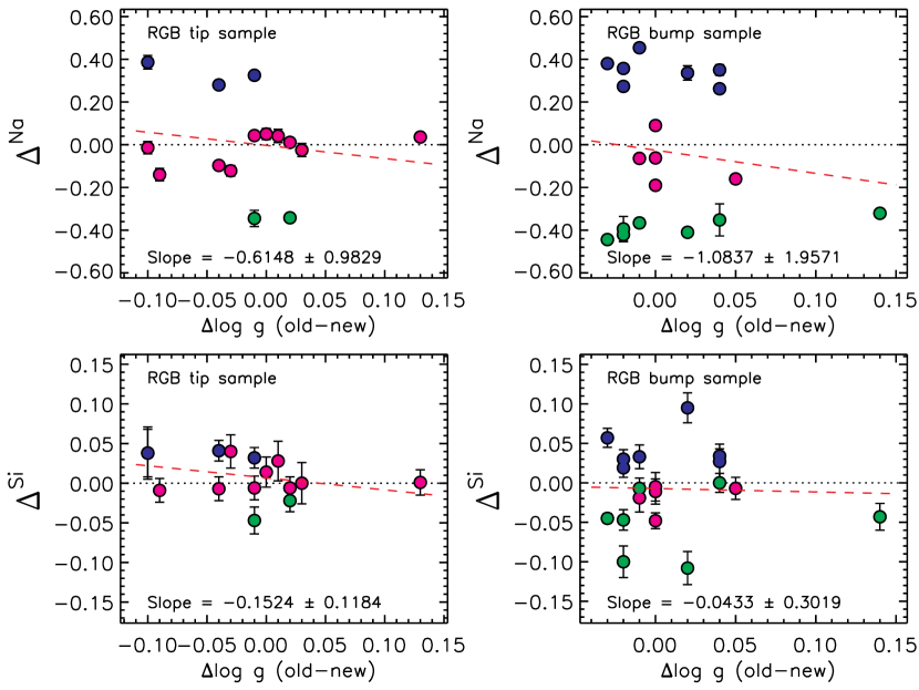
Figure 23: $\Delta^{\rm Na}$ (upper) and $\Delta^{\rm Si}$ (lower) vs. $\Delta$$\log g$ (old = “reference star” values, new = “strictly differential” values) for the RGB tip sample (left) and the RGB bump sample (right). The red dashed line is the linear fit to the data. (These results are obtained when using the reference stars RGB tip = NGC 6752-mg9 and RGB bump = NGC 6752-11.) As in Figure 4, the green, magenta and blue colours represent populations $a$, $b$, and $c$, respectively, from Milone et al. (2013) (see Section 2.1 for details).

On the other hand, for a fixed mass fraction of metals ($Z$), a change in the helium mass fraction ($Y$) will change the hydrogen mass fraction ($X$) and the metal-to-hydrogen ratio, $Z$/$X$, since $X+Y+Z=1$, as we have already noted. If stars in a globular cluster have a constant mass fraction of metals, a He-rich star will appear to be more metal-rich than a He-normal star. The positive correlations we find between $\Delta^{\rm X}$ and $\Delta^{\rm Na}$ are consistent with a He abundance variation since a Na-rich star is expected to be He-rich relative to a Na-poor star.

Bragaglia et al. (2010) examined a large sample of RGB stars in globular clusters and argued that in addition to differences in metallicity, He-rich stars will have subtly different temperatures and RGB bump luminosites. They found evidence for all three effects in their sample. For their primordial (P) and extreme (E) populations, they found [Fe/H]_E $-$ [Fe/H]_P = 0.027 $\pm$ 0.010. The Milone et al. (2013) populations $a$ and $c$ may be regarded as being equivalent to the Carretta et al. (2009b) P and E populations, respectively, and for the RGB bump sample we find $<\Delta^{\rm Fe}_{c}>$ $-$ $<\Delta^{\rm Fe}_{a}>$ = 0.039 $\pm$ 0.015, a value comparable to that of Bragaglia et al. (2010). If we consider all elements, the mean value $<\Delta^{\rm X}_{c}>$ $-$ $<\Delta^{\rm X}_{a}>$ is 0.052 $\pm$ 0.005 ($\sigma$ = 0.019); the smallest difference is for Cr ii (0.031 $\pm$ 0.023) and the largest difference is for Si (0.092 $\pm$ 0.018).

For a fixed value of $Z$, a change in helium abundance from $Y$=0.25 to $Y$=0.28 would produce a change in [X/H] of +0.018 dex. By combining our measurement errors with the expected 0.018 dex abundance variation due to He, we can predict the abundance variations in [X/H]. If we compare these values for each element to the observed variations, we find that the abundance dispersions are, on average, 60% $\pm$ 20% larger than those expected from a change in helium abundance of $\Delta Y$ = 0.03 combined with the measurement uncertainties. Therefore, we tentatively conclude that while the observed abundance variations are qualitatively consistent with a He variation, the magnitudes of the observed variations are unlikely to be explained solely by a He change of $\Delta Y$ = 0.03. To attribute the observed abundance variations entirely to He would require $\Delta Y$ $\simeq$ 0.065, although inclusion of 3D and/or NLTE effects could produce changes in the derived differential abundances. Given the constraints on $\Delta Y$ from photometry (Milone et al., 2013), some process in addition to the He variation may be required to explain the abundance variations that we find.

Before we consider another possibility, we briefly examine the data using ATLAS12 model atmospheres (Castelli, 2005; Kurucz, 2005; Sbordone, 2005). We constructed model atmospheres with $T_{\rm eff}$ = 4800K, $\log g$ = 2.0, $\xi_{t}$ = 2.00 but with two different helium abundances $Y$ = 0.25 and $Y$ = 0.28. We also ensured that the two models had the same mass fraction of metals, $Z$, and thus they have slightly different metallicities $\Delta$[m/H] $\simeq$ 0.015. Using these two model atmospheres, we computed abundances for all elements in three RGB bump stars (9, 10 and 11). These three stars have very similar stellar parameters to the ATLAS12 models but they span a substantial range in Na abundance. For a given element in a given star, we measured the abundance difference when using the $Y$ = 0.28 vs. $Y$ = 0.25 models. The differences are very small and essentially identical for all three stars; the average abundance difference ($Y$ = 0.28 minus $Y$ = 0.25) is 0.001 dex $\pm$ 0.001 dex ($\sigma$ = 0.005 dex). That is, we obtain identical $Z$/$X$ ratios even though the two models have different compositions. Such a result is expected given that the line strength depends only on the ratio of the line opacity to continuous opacity (H- for the program stars), i.e., the $Z$/$X$ ratio.

3.6.4 Inhomogeneous chemical evolution

In the fourth scenario, we assume that the abundance variations are due to chemical inhomogeneities in the pre- or proto-cluster environment. We concentrate on the high statistical significance of the correlations between ($i$) Si and Na, ($ii$) Y and Na and ($iii$) Ca and Na seen in Figures 13, 18, 21 and 22. Such correlations potentially provide great new insight into the origin of the Na abundance variations in NGC 6752, and perhaps in all globular clusters.

The correlation between Si and Na could be attributed to leakage from the Mg-Al chain into ²⁸Si via ²⁷Al(p,$\gamma$)²⁸Si during hydrogen burning at high temperature (Ventura et al., 2011). As noted already, similar conclusions were drawn based on the correlations between Si and Al (Yong et al., 2005) and Si and N (Yong et al., 2008). To our knowledge, such correlations could arise from both the asymptotic giant branch stars (AGB) and the fast rotating massive stars (FRMS) scenarios.

The correlation between Y and Na would suggest that the nucleosynthetic site that produced Na also operated neutron-capture nucleosynthesis. To further explore this issue, we derived chemical abundances for a larger suite of elements expected to participate in neutron-capture reactions (Zn, Y, Zr, Ba, La, Ce, Pr, Nd, Sm, Eu, and Dy). We used only a subset of 10 RGB tip stars with favorable stellar parameters (4250 $\leq T_{\rm eff}\leq$ 4520 K; stars mg8 to mg25) and followed the same procedure described in Sections 2.5 and 2.6, using spectrum synthesis for all lines. (The reference star was NGC 6752-mg9.) For elements with only one measured line (Zn, Zr, Ba, Eu, and Dy), we adopted 0.02 dex as the “fitting error” and used this value as $\sigma_{\rm rand}$ in the error analysis. For comparison, in our analysis of the 5380Å La line in Section 2.5, the average fitting error for the same 10 stars (mg8 to mg25) was 0.016 dex ($\sigma$ = 0.001 dex), and the minimum and maximum values were 0.015 and 0.017 dex, respectively. For the 6645Å Eu line, the average fitting error and minimum and maximum values were 0.017 dex ($\sigma$ = 0.001), 0.014 dex, and 0.018 dex, respectively. Therefore, we regard our choice of 0.02 dex as a somewhat conservative estimate of the fitting error. The line list and abundance differences are presented in Tables 10 and 11. With the exception of Sm, the average errors are comparable to, or smaller than, the measured abundance dispersions. As before, we take this as evidence for a genuine abundance dispersion, of small amplitude, for these elements.

Table 10: Line List for the Neutron-Capture Elements.

Wavelength	Species	L.E.P	$\log gf$	Source
Å		eV
(1)	(2)	(3)	(4)	(5)
4810.53	30.0	4.08	$-$0.15	12
4883.68	39.1	1.08	0.19	1
4900.12	39.1	1.03	0.03	1
4982.13	39.1	1.03	$-$1.32	1
5087.42	39.1	1.08	$-$0.16	1
5119.11	39.1	0.99	$-$1.33	1
5205.72	39.1	1.03	$-$0.28	1
5289.82	39.1	1.03	$-$1.68	1
5402.77	39.1	1.84	$-$0.31	1
5473.38	39.1	1.74	$-$0.78	1
5544.61	39.1	1.74	$-$0.83	1
5728.89	39.1	1.84	$-$1.15	1
5112.27	40.1	1.66	$-$0.85	10
6496.90	56.1	0.60	$-$0.41	11
5114.56	57.1	0.24	$-$1.03	5
5122.99	57.1	0.32	$-$0.91	5
5290.82	57.1	0.00	$-$1.65	4
5301.97	57.1	0.40	$-$0.94	5
5303.53	57.1	0.32	$-$1.35	5
5482.27	57.1	0.00	$-$2.23	5
6262.29	57.1	0.40	$-$1.22	5
6390.48	57.1	0.32	$-$1.41	5
5274.23	58.1	1.04	0.13	8
5330.56	58.1	0.87	$-$0.40	8
6043.37	58.1	1.20	$-$0.48	8
5259.73	59.1	0.63	0.11	3
5322.77	59.1	0.48	$-$0.12	9
4797.15	60.1	0.56	$-$0.69	2
4825.48	60.1	0.18	$-$0.42	2
4914.38	60.1	0.38	$-$0.70	2
4959.12	60.1	0.06	$-$0.80	2
4987.16	60.1	0.74	$-$0.79	2
5063.72	60.1	0.98	$-$0.62	2
5092.79	60.1	0.38	$-$0.61	2
5130.59	60.1	1.30	0.45	2
5132.33	60.1	0.56	$-$0.71	2
5234.19	60.1	0.55	$-$0.51	2
5249.58	60.1	0.98	0.20	2
5293.16	60.1	0.82	0.10	2
5306.46	60.1	0.86	$-$0.97	2
5311.45	60.1	0.98	$-$0.42	2
5319.81	60.1	0.55	$-$0.14	2
5356.97	60.1	1.26	$-$0.28	2
5485.70	60.1	1.26	$-$0.12	2
4815.81	62.1	0.18	$-$0.82	7
4844.21	62.1	0.28	$-$0.89	7
4854.37	62.1	0.38	$-$1.25	7
4913.26	62.1	0.66	$-$0.93	7
6645.10	63.1	1.38	0.12	6
5169.69	66.1	0.10	$-$1.95	13

Table 11: Differential Abundances For Neutron-Capture Elements (Zn, Y, Zr, Ba, La and Ce) in a Subset of RGB Tip Stars (Reference Star = NGC 6752-mg9).

Star	$\Delta^{\rm Zn}$	$\sigma$	$\Delta^{\rm Y}$	$\sigma$	$\Delta^{\rm Zr}$	$\sigma$	$\Delta^{\rm Ba}$	$\sigma$	$\Delta^{\rm La}$	$\sigma$	$\Delta^{\rm Ce}$	$\sigma$
NGC6752-mg8	$-$0.080	0.025	0.020	0.017	0.040	0.021	$-$0.130	0.035	0.025	0.016	0.007	0.024
NGC6752-mg10	$-$0.080	0.025	0.075	0.016	0.070	0.024	0.010	0.039	0.022	0.016	0.017	0.030
NGC6752-mg12	$-$0.060	0.029	$-$0.042	0.020	0.020	0.023	$-$0.030	0.036	$-$0.008	0.026	0.043	0.033
NGC6752-mg15	$-$0.050	0.033	$-$0.014	0.023	0.000	0.024	$-$0.090	0.045	0.003	0.011	0.037	0.035
NGC6752-mg18	$-$0.050	0.033	0.021	0.023	0.020	0.024	$-$0.070	0.044	0.029	0.017	0.047	0.033
NGC6752-mg21	0.010	0.031	0.060	0.020	0.040	0.024	$-$0.020	0.043	0.045	0.019	0.007	0.038
NGC6752-mg22	$-$0.020	0.026	0.045	0.019	0.080	0.021	$-$0.020	0.062	0.039	0.013	0.077	0.020
NGC6752-mg24	$-$0.050	0.037	$-$0.082	0.031	$-$0.020	0.025	$-$0.150	0.065	$-$0.004	0.012	$-$0.053	0.030
NGC6752-mg25	$-$0.130	0.025	$-$0.016	0.024	0.040	0.020	$-$0.150	0.038	$-$0.025	0.010	$-$0.010	0.025

In order to place the above values onto an absolute scale, the absolute abundances we obtain for the reference stars are given below. We caution, however, that the absolute scale has not been critically evaluated (see Section 2.5 for more details).
NGC6752-mg9: A(Zn) = 3.02, A(Y) = 0.49, A(Zr) = 1.34, A(Ba) = 1.02, A(La) = $-$0.33, A(Ce) = 0.00,

Table 12: Differential Abundances For Neutron-Capture Elements (Pr, Nd, Sm, Eu and Dy) in a Subset of RGB Tip Stars (Reference Star = NGC 6752-mg9).

Star	$\Delta^{\rm Pr}$	$\sigma$	$\Delta^{\rm Nd}$	$\sigma$	$\Delta^{\rm Sm}$	$\sigma$	$\Delta^{\rm Eu}$	$\sigma$	$\Delta^{\rm Dy}$	$\sigma$
NGC6752-mg8	0.010	0.011	0.038	0.016	$-$0.037	0.029	0.070	0.021	0.040	0.021
NGC6752-mg10	0.005	0.021	0.029	0.016	$-$0.048	0.029	0.080	0.023	0.110	0.021
NGC6752-mg12	0.010	0.040	0.025	0.012	$-$0.022	0.016	0.030	0.022	0.040	0.021
NGC6752-mg15	$-$0.040	0.016	0.034	0.011	$-$0.010	0.027	0.040	0.025	0.130	0.021
NGC6752-mg18	$-$0.005	0.025	0.019	0.017	$-$0.030	0.025	0.020	0.024	0.070	0.021
NGC6752-mg21	0.005	0.035	0.057	0.014	0.005	0.047	0.050	0.024	0.100	0.021
NGC6752-mg22	0.005	0.022	0.036	0.017	0.010	0.024	0.030	0.021	0.140	0.022
NGC6752-mg24	$-$0.030	0.010	$-$0.012	0.017	$-$0.030	0.026	0.000	0.027	0.090	0.021
NGC6752-mg25	$-$0.045	0.031	$-$0.008	0.017	$-$0.065	0.045	0.000	0.021	0.020	0.021

In order to place the above values onto an absolute scale, the absolute abundances we obtain for the reference stars are given below. We caution, however, that the absolute scale has not been critically evaluated (see Section 2.5 for more details).
NGC6752-mg9: A(Pr) = $-$0.75, A(Nd) = $-$0.02, A(Sm) = $-$0.38, A(Eu) = $-$0.69, A(Dy) = $-$0.25

For these new measurements, we fit the slope to $\Delta^{\rm X}$ vs. $\Delta^{\rm Na}$ as in Section 3.2. We find that the slope is positive for all elements. If we remove the abundance trends with $T_{\rm eff}$ as described in Section 3.4, these results remain unchanged. For Y, La, Nd, and Eu, the results from this new analysis are in agreement with the previous results (at the $<$3$\sigma$ level). In Figure 24, we plot the slope of the fit to $\Delta^{\rm X}$ vs. $\Delta^{\rm Na}$ against the percentage attributed to the $s$-process in the solar system, adopting the solar $s$-process percentages calculated by Bisterzo et al. (2011). In this figure, we also show the slopes when fitting $\Delta^{\rm X}_{\rm T}$ vs. $\Delta^{\rm Na}_{\rm T}$, i.e., after removing the abundance trends with $T_{\rm eff}$. In both cases, the slopes are not of high statistical significance, $<$2$\sigma$ level. If we exclude Y, a possible outlier, the slopes are of even lower statistical significance, $<$1$\sigma$. (The neighboring elements Y and Zr are both members of the first $s$-process peak, so we would not expect their nucleosynthesis histories to be substantially different.) The absence of a significant trend in Figure 24 suggests that the abundance variations are not the result of preferentially introducing more $s$-process material than $r$-process material.

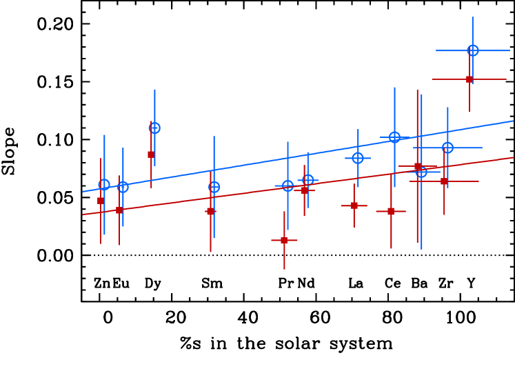
Figure 24: Slope of the fit to $\Delta^{\rm X}$ vs. $\Delta^{\rm Na}$ vs. percentage attributed to the $s$-process in solar system material (using the Bisterzo et al. 2011 values). The red squares are from the “regular” analysis while the blue open circles are fits to the data when abundance trends with $T_{\rm eff}$ have been removed, i.e., slopes of the fits to $\Delta^{\rm X}_{\rm T}$ vs. $\Delta^{\rm Na}_{\rm T}$. Small horizontal offsets ($\pm$ 0.5%) have been applied to aid visibility. Neither slope is significant at the 2$\sigma$ level.

The correlation between Ca and Na requires massive stars to have played a role in the pre- or proto-cluster environment since the synthesis of Ca is believed to occur primarily during O-burning and Si-burning in those objects (Clayton, 2003). That said, the abundances for all elements are positively correlated with the Na abundance, and for any pair of elements heavier than Si, the abundances are positively correlated. Furthermore, the ratios for any pair of elements (e.g., $\Delta^{\rm Ni}$ $-$ $\Delta^{\rm Ca}$ using our terminology) are constant at the 0.036 dex $\pm$ 0.001 dex ($\sigma$ = 0.012) level for the RGB tip sample (excluding Eu, which has considerably larger measurement errors) and essentially identical results are found for the RGB bump sample. Thus, the origin of such correlations demands a source (or sources) capable of synthesis of Na, $\alpha$, Fe-peak and neutron-capture elements and this diverse suite of elements must be synthesized in essentially equal amounts. No individual star can achieve such nucleosynthesis, and therefore, a variety of sources is required.

The underlying assumption in this work, and in other studies, is that the star-to-star light element abundance variations in mono-metallic globular clusters are produced by some source (AGB, FRMS and/or massive binaries) within the duration of star formation in the globular cluster. Such an assumption appears reasonable, although unresolved issues related to nucleosynthesis and enrichment timescales remain (e.g., Fenner et al. 2004; Decressin et al. 2007; Prantzos et al. 2007; Pumo et al. 2008; de Mink et al. 2009; D’Ercole et al. 2012). Regarding the heavy elements, one might also assume that the star-to-star abundance variations and correlations with Na are produced by some source within the duration of star formation in this globular cluster, provided the heavy elements are produced in the same ratios as those already found in the first generation stars. Another possibility is that the heavy element abundance variations and correlations with Na arise because the ejecta from the source that produced Na was diluted into gas with slightly higher [X/H] ratios that entered the cluster while the later generations of stars formed. In this scenario, production of the light elements, including Na, is completely decoupled from production of all elements heavier than Si. Unfortunately, there are no obvious observational tests to distinguish between these two scenarios. We thus regard the “production during cluster formation” and “dilution with pristine material” scenarios as equally valid possibilities for the abundance variations.

The penultimate issue we raise concerns whether the distribution of the heavy element abundances is discrete or continuous. As noted in Section 2.1, Milone et al. (2013) have identified three stellar populations in NGC 6752 based on HST and ground-based Strömgren photometry. The three populations can be found at all evolutionary stages (main sequence, subgiant branch and red giant branch). Additionally, each population exhibits distinct chemical abundance patterns for the light elements (e.g., N, O, Na, Mg and Al). In Figure 11, populations $a$ (green), $b$ (magenta) and $c$ (blue) have distinct $\Delta^{\rm Na}$ abundances. In Figures 14 and 15 (and other figures), we use the same colour scheme to denote the three populations. In general, population $c$ (blue) exhibits a larger (i.e., more positive) value for $\Delta^{\rm X}$ than population $a$ (green), while population $b$ (magenta) lies between populations $a$ and $c$. Such a result is expected given ($i$) the Na abundances of each population and ($ii$) the correlation between $\Delta^{\rm X}$ and $\Delta^{\rm Na}$. Although we have achieved very high precision relative abundance measurements, it is not clear whether the abundance distributions seen in Figures 14 and 15 are consistent with three discrete values in the $\Delta^{\rm X}$ vs. $\Delta^{\rm Y}$ plane, corresponding to the Milone et al. (2013) populations $a$, $b$ and $c$. (That said, it is not obvious whether the Milone et al. 2013 data show three discrete photometric sequences.) Additional studies may be necessary to clarify whether the heavy element abundance distribution is discrete or continuous in this globular cluster.

Finally, we mentioned in the introduction that Sneden (2005) examined the [Ni/Fe] ratio in the context of cluster abundance accuracy limits. There was an apparent limit in $\sigma$[Ni/Fe] at the $\sim$0.06 dex level. For the RGB tip and RGB bump samples, we find $\sigma$($\Delta^{\rm Ni}$ $-$ $\Delta^{\rm Fe}$) = 0.009 and 0.010, respectively, thereby highlighting the great improvement in abundance precision that can be obtained when conducting a strictly differential analysis of high quality spectra.

4 SUMMARY

We have obtained very high precision chemical abundance measurements, $\Delta^{\rm X}$, through a strictly differential analysis of high quality UVES spectra of giant stars in the globular cluster NGC 6752. The measurement uncertainties and average uncertainties for a given element, $<\sigma\Delta^{\rm X}>$, are as low as $\sim$0.01 dex. The observed abundance dispersions, and abundance dispersions about various linear fits (e.g., $\Delta^{\rm X}$ vs. $T_{\rm eff}$ or $\Delta^{\rm X}$ vs. $\Delta^{\rm Y}$), are often considerably larger than the average abundance uncertainty. We find positive correlations between any given element and Na, i.e., $\Delta^{\rm X}$ vs. $\Delta^{\rm Na}$, and indeed for any combination of elements, e.g., $\Delta^{\rm X}$ vs. $\Delta^{\rm Y}$. These correlations are often of high statistical significance ($>$ 5$\sigma$), although we note that the amplitudes of the abundance variations are small. These results are unchanged even after removing abundance trends with $T_{\rm eff}$ and/or when using a different pair of reference stars. Indeed, the likelihood of these results being due to random error is exceedingly small. Therefore, we argue that there is a genuine abundance dispersion in this cluster, at the $\sim$0.03 dex level.

In order to explain these results, we consider four possibilities. The abundance variations and correlations may reflect ($i$) systematic errors in the stellar parameters, ($ii$) star-to-star CNO abundance variations, ($iii$) star-to-star He abundance variations and/or ($iv$) inhomogeneous chemical evolution. In the context of point ($i$), the stellar parameter uncertainties would require substantial increases; our results are seen for all elements (covering a range of ionization potentials and ionization states) and no single change in $T_{\rm eff}$, $\log g$ or $\xi_{t}$ would remove the abundance correlations for all elements. Regarding point ($ii$), predictions by Drake et al. (1993) suggest that for weak lines such as those in this study, using model atmospheres with appropriate CNO abundances will not change our results. Regarding point ($iii$), for a fixed mass fraction of metals ($Z$), an increase in helium abundance ($Y$) would result in a lower hydrogen abundance ($X$) and therefore a higher metal-to-hydrogen ratio, $Z$/$X$. Since Na and He abundances are expected to be correlated, the positive correlations we find between $\Delta^{\rm X}$ vs. $\Delta^{\rm Na}$ are consistent with a He abundance variation (for constant $Z$). Given the current constraints on $\Delta Y$ from photometry (Milone et al., 2013), it is likely that the abundance variations cannot be attributed solely to He. Nevertheless, He abundance variations probably play an important role in producing the abundance variations that we find. Concerning point ($iv$), the correlation between Si and Na could arise from leakage from the Mg-Al chain into Si in either AGB or FRMS. For the neutron-capture elements, there is no significant trend between the slope of the fit to $\Delta^{\rm X}$ vs. $\Delta^{\rm Na}$ when plotted against percentage attributed to the $s$-process in solar system material. Thus, their abundance variations are probably not related to $s$-process production by whatever source produced the light element variations. That all elements are correlated requires a nucleosynthetic source(s) capable of synthesizing Na, $\alpha$, Fe-peak and neutron-capture elements. Additionally, element-to-element ratios (e.g., $\Delta^{\rm Ni}$ $-$ $\Delta^{\rm Ca}$ using our terminology) are constant at the $\sim$0.03 dex level. No individual object can achieve the required nucleosynthesis. We cannot ascertain whether the heavy elements were produced ($a$) within the duration of star formation in this globular cluster or ($b$) by dilution of Na-rich material into gas with slightly higher [X/H] ratios that entered the cluster while the second (and later) generations of stars formed. In summary, our results may be explained by some combination of He abundance variations and inhomogeneous chemical evolution (i.e., metallicity variations). There may be other explanations for the observed abundance variations and correlations. Nevertheless, we encourage similar studies of other globular clusters with no obvious dispersion in Fe-peak elements.

References

- Allende Prieto et al. (2004) Allende Prieto, C., Barklem, P. S., Lambert, D. L., & Cunha, K. 2004, A&A, 420, 183
- Alonso et al. (1999) Alonso, A., Arribas, S., & Martínez-Roger, C. 1999, A&AS, 140, 261
- Alves-Brito et al. (2010) Alves-Brito, A., Meléndez, J., Asplund, M., Ramírez, I., & Yong, D. 2010, A&A, 513, A35
- Alves-Brito et al. (2012) Alves-Brito, A., Yong, D., Meléndez, J., Vásquez, S., & Karakas, A. I. 2012, A&A, 540, A3
- Asplund (2005) Asplund, M. 2005, ARA&A, 43, 481
- Asplund et al. (2009) Asplund, M., Grevesse, N., Sauval, A. J., & Scott, P. 2009, ARA&A, 47, 481
- Barklem et al. (2005) Barklem, P. S., Christlieb, N., Beers, T. C., Hill, V., Bessell, M. S., Holmberg, J., Marsteller, B., Rossi, S., Zickgraf, F., & Reimers, D. 2005, A&A, 439, 129
- Bekki (2011) Bekki, K. 2011, MNRAS, 412, 2241
- Biemont et al. (1991) Biemont, E., Baudoux, M., Kurucz, R. L., Ansbacher, W., & Pinnington, E. H. 1991, A&A, 249, 539
- Biémont et al. (2011) Biémont, É., Blagoev, K., Engström, L., Hartman, H., Lundberg, H., Malcheva, G., Nilsson, H., Whitehead, R. B., Palmeri, P., & Quinet, P. 2011, MNRAS, 414, 3350
- Bisterzo et al. (2011) Bisterzo, S., Gallino, R., Straniero, O., Cristallo, S., & Käppeler, F. 2011, MNRAS, 418, 284
- Blackwell et al. (1986) Blackwell, D. E., Booth, A. J., Haddock, D. J., Petford, A. D., & Leggett, S. K. 1986, MNRAS, 220, 549
- Blackwell et al. (1979a) Blackwell, D. E., Ibbetson, P. A., Petford, A. D., & Shallis, M. J. 1979a, MNRAS, 186, 633
- Blackwell et al. (1995) Blackwell, D. E., Lynas-Gray, A. E., & Smith, G. 1995, A&A, 296, 217
- Blackwell et al. (1979b) Blackwell, D. E., Petford, A. D., & Shallis, M. J. 1979b, MNRAS, 186, 657
- Blackwell et al. (1980) Blackwell, D. E., Petford, A. D., Shallis, M. J., & Simmons, G. J. 1980, MNRAS, 191, 445
- Bragaglia et al. (2010) Bragaglia, A., Carretta, E., Gratton, R., D’Orazi, V., Cassisi, S., & Lucatello, S. 2010, A&A, 519, A60
- Buonanno et al. (1986) Buonanno, R., Caloi, V., Castellani, V., Corsi, C., Fusi Pecci, F., & Gratton, R. 1986, A&AS, 66, 79
- Campbell et al. (2013) Campbell, S. W., D’Orazi, V., Yong, D., Constantino, T. N., Lattanzio, J. C., Stancliffe, R. J., Angelou, G. C., Wylie-de Boer, E. C., & Grundahl, F. 2013, Nature, 498, 198
- Cannon et al. (1998) Cannon, R. D., Croke, B. F. W., Bell, R. A., Hesser, J. E., & Stathakis, R. A. 1998, MNRAS, 298, 601
- Carretta et al. (2009a) Carretta, E., Bragaglia, A., Gratton, R., D’Orazi, V., & Lucatello, S. 2009a, A&A, 508, 695
- Carretta et al. (2010) Carretta, E., Bragaglia, A., Gratton, R. G., Lucatello, S., Bellazzini, M., Catanzaro, G., Leone, F., Momany, Y., Piotto, G., & D’Orazi, V. 2010, ApJ, 714, L7
- Carretta et al. (2009b) Carretta, E., Bragaglia, A., Gratton, R. G., Lucatello, S., Catanzaro, G., Leone, F., Bellazzini, M., Claudi, R., D’Orazi, V., Momany, Y., Ortolani, S., Pancino, E., Piotto, G., Recio-Blanco, A., & Sabbi, E. 2009b, A&A, 505, 117
- Carretta et al. (2005) Carretta, E., Gratton, R. G., Lucatello, S., Bragaglia, A., & Bonifacio, P. 2005, A&A, 433, 597
- Carretta et al. (2011) Carretta, E., Lucatello, S., Gratton, R. G., Bragaglia, A., & D’Orazi, V. 2011, A&A, 533, A69
- Castelli (2005) Castelli, F. 2005, Memorie della Societa Astronomica Italiana Supplementi, 8, 25
- Castelli & Kurucz (2003) Castelli, F. & Kurucz, R. L. 2003, in IAU Symp. 210, Modelling of Stellar Atmospheres, ed. N. Piskunov, W. W. Weiss, & D. F. Gray (San Francisco, CA: ASP), A20
- Clayton (2003) Clayton, D. 2003, Handbook of Isotopes in the Cosmos
- Cohen et al. (2011) Cohen, J. G., Huang, W., & Kirby, E. N. 2011, ApJ, 740, 60
- Cohen & Kirby (2012) Cohen, J. G. & Kirby, E. N. 2012, ApJ, 760, 86
- Cohen et al. (2010) Cohen, J. G., Kirby, E. N., Simon, J. D., & Geha, M. 2010, ApJ, 725, 288
- Conroy & Spergel (2011) Conroy, C. & Spergel, D. N. 2011, ApJ, 726, 36
- de Mink et al. (2009) de Mink, S. E., Pols, O. R., Langer, N., & Izzard, R. G. 2009, A&A, 507, L1
- Decressin et al. (2007) Decressin, T., Meynet, G., Charbonnel, C., Prantzos, N., & Ekström, S. 2007, A&A, 464, 1029
- Dekker et al. (2000) Dekker, H., D’Odorico, S., Kaufer, A., Delabre, B., & Kotzlowski, H. 2000, in Society of Photo-Optical Instrumentation Engineers (SPIE) Conference Series, Vol. 4008, Society of Photo-Optical Instrumentation Engineers (SPIE) Conference Series, ed. M. Iye & A. F. Moorwood, 534–545
- Den Hartog et al. (2003) Den Hartog, E. A., Lawler, J. E., Sneden, C., & Cowan, J. J. 2003, ApJS, 148, 543
- D’Ercole et al. (2012) D’Ercole, A., D’Antona, F., Carini, R., Vesperini, E., & Ventura, P. 2012, MNRAS, 423, 1521
- D’Ercole et al. (2008) D’Ercole, A., Vesperini, E., D’Antona, F., McMillan, S. L. W., & Recchi, S. 2008, MNRAS, 391, 825
- D’Orazi et al. (2013) D’Orazi, V., Campbell, S. W., Lugaro, M., Lattanzio, J. C., Pignatari, M., & Carretta, E. 2013, MNRAS in press (arXiv:1304.7009)
- D’Orazi et al. (2010) D’Orazi, V., Lucatello, S., Gratton, R., Bragaglia, A., Carretta, E., Shen, Z., & Zaggia, S. 2010, ApJ, 713, L1
- Drake et al. (1993) Drake, J. J., Plez, B., & Smith, V. V. 1993, ApJ, 412, 612
- Fenner et al. (2004) Fenner, Y., Campbell, S., Karakas, A. I., Lattanzio, J. C., & Gibson, B. K. 2004, MNRAS, 353, 789
- Fuhr & Wiese (2009) Fuhr, J. R. & Wiese, W. L. 2009, Atomic Transition Probabilities, published in the CRC Handbook of Chemistry and Physics, 90th Edition, ed. Lide, D. R., CRC Press, Inc., Boca Raton, FL, 10
- Gratton et al. (2004) Gratton, R., Sneden, C., & Carretta, E. 2004, ARA&A, 42, 385
- Gratton et al. (2001) Gratton, R. G., Bonifacio, P., Bragaglia, A., Carretta, E., Castellani, V., Centurion, M., Chieffi, A., Claudi, R., Clementini, G., D’Antona, F., Desidera, S., François, P., Grundahl, F., Lucatello, S., Molaro, P., Pasquini, L., Sneden, C., Spite, F., & Straniero, O. 2001, A&A, 369, 87
- Gratton et al. (2005) Gratton, R. G., Bragaglia, A., Carretta, E., de Angeli, F., Lucatello, S., Piotto, G., & Recio Blanco, A. 2005, A&A, 440, 901
- Gratton et al. (2012) Gratton, R. G., Carretta, E., & Bragaglia, A. 2012, A&A Rev., 20, 50
- Gratton et al. (2010) Gratton, R. G., Carretta, E., Bragaglia, A., Lucatello, S., & D’Orazi, V. 2010, A&A, 517, A81
- Gratton et al. (2003) Gratton, R. G., Carretta, E., Claudi, R., Lucatello, S., & Barbieri, M. 2003, A&A, 404, 187
- Grundahl et al. (2002) Grundahl, F., Briley, M., Nissen, P. E., & Feltzing, S. 2002, A&A, 385, L14
- Grundahl et al. (1999) Grundahl, F., Catelan, M., Landsman, W. B., Stetson, P. B., & Andersen, M. I. 1999, ApJ, 524, 242
- Gustafsson et al. (1975) Gustafsson, B., Bell, R. A., Eriksson, K., & Nordlund, A. 1975, A&A, 42, 407
- Gustafsson et al. (2008) Gustafsson, B., Edvardsson, B., Eriksson, K., Jørgensen, U. G., Nordlund, Å., & Plez, B. 2008, A&A, 486, 951
- Harris (1996) Harris, W. E. 1996, AJ, 112, 1487
- Ivans et al. (2001) Ivans, I. I., Kraft, R. P., Sneden, C., Smith, G. H., Rich, R. M., & Shetrone, M. 2001, AJ, 122, 1438
- Ivans et al. (2006) Ivans, I. I., Simmerer, J., Sneden, C., Lawler, J. E., Cowan, J. J., Gallino, R., & Bisterzo, S. 2006, ApJ, 645, 613
- Ivarsson et al. (2001) Ivarsson, S., Litzén, U., & Wahlgren, G. M. 2001, Phys. Scr, 64, 455
- Jefferys et al. (1988) Jefferys, W. H., Fitzpatrick, M. J., & McArthur, B. E. 1988, Celestial Mechanics, 41, 39
- Johnson & Pilachowski (2010) Johnson, C. I. & Pilachowski, C. A. 2010, ApJ, 722, 1373
- Johnson (2002) Johnson, J. A. 2002, ApJS, 139, 219
- Kraft (1994) Kraft, R. P. 1994, PASP, 106, 553
- Kurucz & Bell (1995) Kurucz, R. & Bell, B. 1995, Atomic Line Data (R.L. Kurucz and B. Bell) Kurucz CD-ROM No. 23. Cambridge, Mass.: Smithsonian Astrophysical Observatory, 1995., 23
- Kurucz (2005) Kurucz, R. L. 2005, Memorie della Societa Astronomica Italiana Supplementi, 8, 14
- Lawler et al. (2001a) Lawler, J. E., Bonvallet, G., & Sneden, C. 2001a, ApJ, 556, 452
- Lawler et al. (2006) Lawler, J. E., Den Hartog, E. A., Sneden, C., & Cowan, J. J. 2006, ApJS, 162, 227
- Lawler et al. (2009) Lawler, J. E., Sneden, C., Cowan, J. J., Ivans, I. I., & Den Hartog, E. A. 2009, ApJS, 182, 51
- Lawler et al. (2001b) Lawler, J. E., Wickliffe, M. E., den Hartog, E. A., & Sneden, C. 2001b, ApJ, 563, 1075
- Li et al. (2007) Li, R., Chatelain, R., Holt, R. A., Rehse, S. J., Rosner, S. D., & Scholl, T. J. 2007, Phys. Scr, 76, 577
- Lind et al. (2011a) Lind, K., Asplund, M., Barklem, P. S., & Belyaev, A. K. 2011a, A&A, 528, A103
- Lind et al. (2012) Lind, K., Bergemann, M., & Asplund, M. 2012, MNRAS, 427, 50
- Lind et al. (2011b) Lind, K., Charbonnel, C., Decressin, T., Primas, F., Grundahl, F., & Asplund, M. 2011b, A&A, 527, A148
- Ljung et al. (2006) Ljung, G., Nilsson, H., Asplund, M., & Johansson, S. 2006, A&A, 456, 1181
- Lodders (2003) Lodders, K. 2003, ApJ, 591, 1220
- Mackey & Broby Nielsen (2007) Mackey, A. D. & Broby Nielsen, P. 2007, MNRAS, 379, 151
- Marcolini et al. (2009) Marcolini, A., Gibson, B. K., Karakas, A. I., & Sánchez-Blázquez, P. 2009, MNRAS, 395, 719
- Marino et al. (2009) Marino, A. F., Milone, A. P., Piotto, G., Villanova, S., Bedin, L. R., Bellini, A., & Renzini, A. 2009, A&A, 505, 1099
- Marino et al. (2011) Marino, A. F., Sneden, C., Kraft, R. P., Wallerstein, G., Norris, J. E., da Costa, G., Milone, A. P., Ivans, I. I., Gonzalez, G., Fulbright, J. P., Hilker, M., Piotto, G., Zoccali, M., & Stetson, P. B. 2011, A&A, 532, A8
- McWilliam et al. (1995) McWilliam, A., Preston, G. W., Sneden, C., & Searle, L. 1995, AJ, 109, 2757
- Meléndez et al. (2009) Meléndez, J., Asplund, M., Gustafsson, B., & Yong, D. 2009, ApJ, 704, L66
- Meléndez et al. (2012) Meléndez, J., Bergemann, M., Cohen, J. G., Endl, M., Karakas, A. I., Ramírez, I., Cochran, W. D., Yong, D., MacQueen, P. J., Kobayashi, C., & Asplund, M. 2012, A&A, 543, A29
- Meléndez & Cohen (2009) Meléndez, J. & Cohen, J. G. 2009, ApJ, 699, 2017
- Mészáros & Allende Prieto (2013) Mészáros, S. & Allende Prieto, C. 2013, MNRAS
- Milone et al. (2009) Milone, A. P., Bedin, L. R., Piotto, G., & Anderson, J. 2009, A&A, 497, 755
- Milone et al. (2013) Milone, A. P., Marino, A. F., Piotto, G., Bedin, L. R., Anderson, J., Aparicio, A., Bellini, A., Cassisi, S., D’Antona, F., Grundahl, F., Monelli, M., & Yong, D. 2013, ApJ in press (arXiv:1301.7044)
- Milone et al. (2012) Milone, A. P., Piotto, G., Bedin, L. R., King, I. R., Anderson, J., Marino, A. F., Bellini, A., Gratton, R., Renzini, A., Stetson, P. B., Cassisi, S., Aparicio, A., Bragaglia, A., Carretta, E., D’Antona, F., Di Criscienzo, M., Lucatello, S., Monelli, M., & Pietrinferni, A. 2012, ApJ, 744, 58
- Mucciarelli et al. (2012) Mucciarelli, A., Bellazzini, M., Ibata, R., Merle, T., Chapman, S. C., Dalessandro, E., & Sollima, A. 2012, MNRAS, 426, 2889
- Nissen & Schuster (2010) Nissen, P. E. & Schuster, W. J. 2010, A&A, 511, L10
- Nissen & Schuster (2011) —. 2011, A&A, 530, A15
- Norris & Da Costa (1995) Norris, J. E. & Da Costa, G. S. 1995, ApJ, 447, 680
- Origlia et al. (2011) Origlia, L., Rich, R. M., Ferraro, F. R., Lanzoni, B., Bellazzini, M., Dalessandro, E., Mucciarelli, A., Valenti, E., & Beccari, G. 2011, ApJ, 726, L20
- Penny & Dickens (1986) Penny, A. J. & Dickens, R. J. 1986, MNRAS, 220, 845
- Piotto (2009) Piotto, G. 2009, in IAU Symposium, Vol. 258, IAU Symposium, ed. E. E. Mamajek, D. R. Soderblom, & R. F. G. Wyse, 233–244
- Piotto et al. (2005) Piotto, G., Villanova, S., Bedin, L. R., Gratton, R., Cassisi, S., Momany, Y., Recio-Blanco, A., Lucatello, S., Anderson, J., King, I. R., Pietrinferni, A., & Carraro, G. 2005, ApJ, 621, 777
- Popper (1947) Popper, D. M. 1947, ApJ, 105, 204
- Prantzos et al. (2007) Prantzos, N., Charbonnel, C., & Iliadis, C. 2007, A&A, 470, 179
- Prochaska et al. (2000) Prochaska, J. X., Naumov, S. O., Carney, B. W., McWilliam, A., & Wolfe, A. M. 2000, AJ, 120, 2513
- Pumo et al. (2008) Pumo, M. L., D’Antona, F., & Ventura, P. 2008, ApJ, 672, L25
- Ramírez et al. (2010) Ramírez, I., Asplund, M., Baumann, P., Meléndez, J., & Bensby, T. 2010, A&A, 521, A33
- Ramírez et al. (2012) Ramírez, I., Meléndez, J., & Chanamé, J. 2012, ApJ, 757, 164
- Ramírez & Cohen (2002) Ramírez, S. V. & Cohen, J. G. 2002, AJ, 123, 3277
- Ramírez & Cohen (2003) —. 2003, AJ, 125, 224
- Roederer & Lawler (2012) Roederer, I. U. & Lawler, J. E. 2012, ApJ, 750, 76
- Roederer et al. (2011) Roederer, I. U., Marino, A. F., & Sneden, C. 2011, ApJ, 742, 37
- Rood & Crocker (1985) Rood, R. T. & Crocker, D. A. 1985, in European Southern Observatory Conference and Workshop Proceedings, Vol. 21, European Southern Observatory Conference and Workshop Proceedings, ed. I. J. Danziger, F. Matteucci, & K. Kjar, 61–69
- Saviane et al. (2012) Saviane, I., Da Costa, G. S., Held, E. V., Sommariva, V., Gullieuszik, M., Barbuy, B., & Ortolani, S. 2012, A&A in press (arXiv:1202.1304)
- Sbordone (2005) Sbordone, L. 2005, Memorie della Societa Astronomica Italiana Supplementi, 8, 61
- Sbordone et al. (2011) Sbordone, L., Salaris, M., Weiss, A., & Cassisi, S. 2011, A&A, 534, A9
- Simmerer et al. (2013) Simmerer, J., Ivans, I. I., Filler, D., Francois, P., Charbonnel, C., Monier, R., & James, G. 2013, ApJ, 764, L7
- Smith (1987) Smith, G. H. 1987, PASP, 99, 67
- Sneden (1973) Sneden, C. 1973, ApJ, 184, 839
- Sneden (2005) Sneden, C. 2005, in IAU Symposium, Vol. 228, From Lithium to Uranium: Elemental Tracers of Early Cosmic Evolution, ed. V. Hill, P. François, & F. Primas, 337–344
- Sneden et al. (2000) Sneden, C., Johnson, J., Kraft, R. P., Smith, G. H., Cowan, J. J., & Bolte, M. S. 2000, ApJ, 536, L85
- Sneden et al. (1997) Sneden, C., Kraft, R. P., Shetrone, M. D., Smith, G. H., Langer, G. E., & Prosser, C. F. 1997, AJ, 114, 1964
- Sneden et al. (2009) Sneden, C., Lawler, J. E., Cowan, J. J., Ivans, I. I., & Den Hartog, E. A. 2009, ApJS, 182, 80
- Sobeck et al. (2011) Sobeck, J. S., Kraft, R. P., Sneden, C., Preston, G. W., Cowan, J. J., Smith, G. H., Thompson, I. B., Shectman, S. A., & Burley, G. S. 2011, AJ, 141, 175
- Stetson & Pancino (2008) Stetson, P. B. & Pancino, E. 2008, PASP, 120, 1332
- Strömgren et al. (1982) Strömgren, B., Gustafsson, B., & Olsen, E. H. 1982, PASP, 94, 5
- VandenBerg et al. (2000) VandenBerg, D. A., Swenson, F. J., Rogers, F. J., Iglesias, C. A., & Alexander, D. R. 2000, ApJ, 532, 430
- Ventura et al. (2011) Ventura, P., Carini, R., & D’Antona, F. 2011, MNRAS, 415, 3865
- Ventura & D’Antona (2005) Ventura, P. & D’Antona, F. 2005, ApJ, 635, L149
- Villanova & Geisler (2011) Villanova, S. & Geisler, D. 2011, A&A, 535, A31
- Villanova et al. (2010) Villanova, S., Geisler, D., & Piotto, G. 2010, ApJ, 722, L18
- Villanova et al. (2009) Villanova, S., Piotto, G., & Gratton, R. G. 2009, A&A, 499, 755
- Wickliffe et al. (2000) Wickliffe, M. E., Lawler, J. E., & Nave, G. 2000, J. Quant. Spec. Radiat. Transf., 66, 363
- Yong & Grundahl (2008) Yong, D. & Grundahl, F. 2008, ApJ, 672, L29
- Yong et al. (2008) Yong, D., Grundahl, F., Johnson, J. A., & Asplund, M. 2008, ApJ, 684, 1159
- Yong et al. (2003) Yong, D., Grundahl, F., Lambert, D. L., Nissen, P. E., & Shetrone, M. D. 2003, A&A, 402, 985
- Yong et al. (2005) Yong, D., Grundahl, F., Nissen, P. E., Jensen, H. R., & Lambert, D. L. 2005, A&A, 438, 875