Radiative corrections to the composite Higgs mass from a gluon partner

Abstract

In composite Higgs models light fermionic top partners often play an important role in obtaining a 126 GeV Higgs mass. The presence of these top partners implies that coloured vector mesons, or massive gluon partners, most likely exist. Since the coupling between the top partners and gluon partners can be large there are then sizeable two-loop contributions to the composite Higgs mass. We compute the radiative correction to the Higgs mass from a gluon partner in the minimal composite Higgs model and show that the Higgs mass is in fact reduced. This allows the top partner masses to be increased, easing the tension between having a light composite Higgs and heavy top partners.

1 Introduction

The recent discovery of the Higgs boson at the Large Hadron Collider (LHC) [1, 2, 3] confirms that the Higgs mechanism is responsible for spontaneously breaking electroweak symmetry in the Standard Model (SM). However, the question of whether the Higgs sector is natural or not remains to be answered. The two most appealing solutions for stabilising the weak scale are supersymmetry (see ref. [4] for a review) and compositeness [5, 6]. Both are now constrained by measurements of the Higgs mass and its couplings, which have led to consequences for the spectrum of exotic states predicted in these two scenarios. In supersymmetric models the radiative corrections from coloured states, such as the stop and gluino, have been extensively studied in the literature and shown to have an important effect on tuning in the Higgs sector. Combined with the lower limits on sparticle masses from the LHC, the conclusion is that supersymmetric models are now tuned to below the 5$\%$ level [7].

Exotic coloured states also exist in composite Higgs models and can similarly play an important role in determining the Higgs mass. In many of these models the SM Higgs doublet is identified with Nambu-Goldstone modes, arising from the spontaneous breaking of a global symmetry group $G$ to a subgroup $H$ due to some strong dynamics. However, the original global symmetry is also explicitly broken via mixing between operators in the strongly coupled sector and elementary fields in the SM sector, as the latter need not come in complete representations of $G$. Hence a Coleman-Weinberg type potential is generated, leading to dynamical electroweak symmetry breaking and a mass for the Higgs boson [8].

A key component in such models is the existence of composite, fermionic top partner resonances in the low energy spectrum. They are required to facilitate a strong coupling between the top quark and the composite Higgs (through substantial mixing between composite and elementary states in the top sector) and, often, to break electroweak symmetry in the first place. The scale of the Higgs mass is typically set by these top partner masses so, to provide a Higgs mass of around 126 GeV [9, 10, 11, 12, 13], the top partners cannot be too heavy. Including such coloured fermionic resonances generically implies that there will also be coloured vector meson resonances in the low energy spectrum. This follows because, even though a complete description of the underlying dynamics of the strong sector remains unknown, the constituents of the strong sector must be coloured in order to produce top partner bound states charged under $SU(3)$ colour. Consequently, the strong sector is also expected to produce coloured vector mesons that necessarily couple to any top partner bound state. We will refer to these states as gluon partners. Indeed, if the strong sector contains a fermionic operator ${\cal O}_{\psi}$, in the fundamental representation of $SU(3)$ so as to produce top partners, one can always write down a vector operator $\bar{{\cal O}_{\psi}}\gamma^{\mu}{{\cal O}}_{\psi}$ in the adjoint representation of $SU(3)$. Equivalently, in the five-dimensional (5D) version of these composite Higgs models [14, 15, 16, 17, 18] the gluon partners are simply the Kaluza-Klein gluons, which are required by 5D gauge invariance if the SM fermions are located in the bulk.

Thus far the contribution of gluon partners to the Higgs mass has been neglected. Since they only couple to the Higgs through the top partners, the size of the correction to the Higgs mass will be proportional to the gluon partner-top partner coupling, $\alpha_{G}$. This coupling can be estimated either through direct calculations in the 5D theory [19] or via holographic techniques [20]. In both instances the coupling is large, hence the contribution to the Higgs mass is expected to be sizeable.

In this paper we explicitly compute the leading order correction and do indeed find it to be important. Specifically, we calculate the one-loop correction to the two-point function of (Dirac) top partners coming from a massive gluon partner. This first result is model independent but, to quantify the effect on the Higgs mass, we apply it to the specific example of the MCHM₅. Interestingly, we find that the Higgs mass is decreased in this particular model, thereby easing some of the tension between the tuning in composite Higgs models and the non-observation of coloured top partners. For a gluon partner of mass 3 TeV, a spontaneous global symmetry breaking scale of about 750 GeV and with the Higgs mass fixed at 126 GeV, the top partners are about 10% heavier than in the uncorrected model.

The rest of this paper is organised as follows. In section 2 we consider gluon partners in a general composite Higgs model. The one-loop radiative correction from a gluon partner to the two-point function is first estimated in the large $N$ limit and then the exact calculation is performed with the final result expressed in integral form. The exact result is used in section 3 to compute the contribution to the composite Higgs mass in the MCHM₅. The concluding remarks are presented in section 4. In appendix A we use the holographic basis to estimate the size of the radiative correction, and in appendix B we list the Passarino-Veltman integral expressions utilised earlier in the paper.

2 Gluon partners and the composite Higgs mass

Many composite Higgs models consists of a strong sector that is responsible for producing a set of Nambu-Goldstone bosons, a combination of which is identified with the Higgs boson, $h$. The strong sector is joined by an elementary sector containing the SM fermions and gauge bosons, and the two sectors are assumed to mix only through bilinear couplings

$${\cal L}_{\rm mix}=\bar{q}_{L}{\cal O}_{R}+\bar{t}_{R}{\cal O}_{L}+A_{g}^{\mu}{\cal J}_{\mu}+\ldots$$ (2.1)

where the elementary fields $q_{L},t_{R}$ and $A_{g}$ are the left handed top quark doublet, right handed top and gluon respectively. We have only included the fermionic operators ${\cal O}_{L/R}$ and the strong sector $SU(3)$ colour current ${\cal J}$; the dots represent other bilinear couplings which will not be considered here, such as those for the light fermions.

Integrating out the strong sector results in an effective Lagrangian for the top-Higgs sector [14]

$${\cal L}_{\rm eff}={} \bar{t}_{L}\not{p}\left[\Pi_{L}^{0}(p^{2})+{\cal Y}_{L}(h/f)\Pi_{L}^{h}(p^{2})\right]t_{L}+\bar{t}_{R}\not{p}\left[\Pi_{R}^{0}(p^{2})+{\cal Y}_{R}(h/f)\Pi_{R}^{h}(p^{2})\right]t_{R}+{}$$

$$\left[\bar{t}_{L}{\cal Y}_{M}(h/f)M(p^{2})t_{R}+\mbox{h.c.}\right],$$ (2.2)

where $f$ is the Nambu-Goldstone boson decay constant. The functions $\Pi$ and $M$ are determined by two-point functions of the fermionic operators

$$\not{p}\Pi_{L/R}(p^{2}) \sim\langle{\cal O}_{L/R}(p)\bar{{\cal O}}_{L/R}(-p)\rangle, M(p^{2}) \sim\langle{\cal O}_{L}(p)\bar{{\cal O}}_{R}(-p)\rangle,$$ (2.3)

up to a factor of $+1$ in $\Pi^{0}$ coming from the usual SM kinetic term (i.e. $\Pi^{0}\sim 1+\langle{\cal O}\bar{{\cal O}}\rangle$). Assuming the strong sector is a large $N$ gauge theory and working to leading order in $1/N$, one can write these two-point functions as a sum over narrow, top partner resonances, $Q_{n}$, to find

$$\Pi_{L/R}(p^{2}) =\sum_{n=1}^{\infty}\frac{a_{n}|F^{L/R}_{n}|^{2}}{p^{2}-m_{Q_{n}}^{2}}, M(p^{2}) =\sum_{n=1}^{\infty}\frac{b_{n}F^{L}_{n}F^{R}_{n}{}^{*}m_{Q_{n}}}{p^{2}-m_{Q_{n}}^{2}},$$ (2.4)

for masses $m_{Q_{n}}$, constant form factors $F_{n}$ and where the coefficients $a_{n},b_{n}$ are derived from the group structure of any particular model. Their precise form and that of their prefactors, the functions ${\cal Y}(h/f)$ of the Higgs fields, are determined by the details of the global symmetry breaking pattern and the representations into which the top quarks are embedded. However, they can always be split into those components that are sensitive to the Higgs vacuum expectation value (VEV) and those that are not, hence ${\cal Y}_{L}(0)={\cal Y}_{R}(0)={\cal Y}_{M}(0)=0$.

Since the top quarks do not make up full representations of the global symmetry group in the strong sector, the symmetry is explicitly broken and a potential can be generated for the erstwhile Nambu-Goldstone bosons. At one loop the potential from the top sector is given by

$$V_{\rm eff}(h)=-2N_{c}\int\frac{\mathrm{d}^{4}p_{E}}{(2\pi)^{4}}\,\ln\left(-p_{E}^{2}\left[\Pi^{0}_{L}(p_{E}^{2})+{\cal Y}_{L}(h/f)\Pi_{L}^{h}(p_{E}^{2})\right]\left[\Pi^{0}_{R}(p_{E}^{2})+{\cal Y}_{R}(h/f)\Pi_{R}^{h}(p_{E}^{2})\right]\right.$$

$$\left.{}-\left|{\cal Y}_{M}(h/f)M(p_{E}^{2})\right|^{2}\right),$$ (2.5)

where $N_{c}=3$ is the QCD colour factor and the integral is performed over Euclidean momentum $p_{E}$. Expanding the logarithm and discarding the constant term gives an approximate form for the potential

$$V_{\rm eff}(h)\approx-6\int\frac{\mathrm{d}^{4}p_{E}}{(2\pi)^{4}}\,\left[\frac{{\cal Y}_{L}(h/f)\Pi_{L}^{h}(p_{E}^{2})}{\Pi^{0}_{L}(p_{E}^{2})}+\frac{{\cal Y}_{R}(h/f)\Pi_{R}^{h}(p_{E}^{2})}{\Pi^{0}_{R}(p_{E}^{2})}+\frac{\left|{\cal Y}_{M}(h/f)M(p_{E}^{2})\right|^{2}}{p_{E}^{2}\Pi_{L}^{0}(p_{E}^{2})\Pi_{R}^{0}(p_{E}^{2})}\right.$$

$$\left.{}-\left(\frac{{\cal Y}_{L}(h/f)\Pi_{L}^{h}(p_{E}^{2})}{2\Pi^{0}_{L}(p_{E}^{2})}\right)^{2}-\left(\frac{{\cal Y}_{R}(h/f)\Pi_{R}^{h}(p_{E}^{2})}{2\Pi^{0}_{R}(p_{E}^{2})}\right)^{2}\right],$$ (2.6)

which can be considered an expansion in ${\cal Y}(h/f)$ (corresponding to a small Higgs VEV) or an expansion in $\Pi^{h}_{L/R}$ and $M$ (corresponding to weak mixing between elementary and composite degrees of freedom).

2.1 Gluon partner contributions

The operators ${\cal O}_{L}$ and ${\cal O}_{R}$ in the strong sector, which are required to mix with the top quark, guarantee the existence of top partners in this framework. However, as argued in the introduction, they are typically accompanied by massive, coloured vector meson resonances, or gluon partners. These are associated with the strong sector current operator ${\cal J}$ as, at leading order in $1/N$, the two-point function $\langle{\cal J}{\cal J}\rangle$ can be written as a sum over narrow gluon resonances, $G_{n}$, much like the two-point functions $\Pi$ and $M$.

Because the Higgs is colour neutral, any correction to its mass from gluon partners must enter, at two-loop order, through the two-point functions of ${\cal O}_{L}$ and ${\cal O}_{R}$. This means the effect can be accounted for by calculating the gluon partner corrections to the functions $M$ and $\Pi$, defined in eq. (2.4) in the large $N$ limit. A naive large $N$ analysis suggests that the correction is not important because it depends on a ${\cal O}{\cal O}{\cal J}$ coupling in the strong sector, which scales like $1/\sqrt{N}$. However, this is only a scaling dependence and ignores the prefactor for the coupling, which we will now show is large. To estimate the importance of the correction more accurately we will use the AdS/CFT correspondence to estimate the strength of couplings in the strong sector, then use large $N$ results to estimate the amplitudes of the relevant diagrams.

In theories of warped extra dimensions one can relate the $N$ appearing in the large $N$ CFT expansion with the 5D gauge couplings using [20]

$$\frac{1}{\kappa_{i}N}=\frac{g_{5,i}^{2}k}{16\pi^{2}}=\frac{g_{i}^{2}}{16\pi^{2}}\ln\left(\frac{\Lambda_{\rm UV}}{\Lambda_{\rm IR}}\right),$$ (2.7)

where $k$ is the curvature scale of the 5D warped AdS space, $g_{5,i}$ a bulk gauge coupling, $g_{i}$ a four-dimensional (4D) gauge coupling and $\kappa_{i}$ a numerical factor distinguishing between different gauge groups. We have also made use of the relation between 5D and 4D gauge couplings $g_{5,i}^{2}k=g_{i}^{2}\ln{(\Lambda_{\rm UV}/\Lambda_{\rm IR})}$, which includes the logarithmic running between the UV and the IR scales. The expression (2.7) can be used to provide quantitative information about the strength of the couplings between resonances in the strong sector.

To estimate the coupling between the top partner and the gluon partner, we first use the $SU(3)$ gauge coupling to obtain the value for $\kappa_{3}N$. Using (2.7) one finds

$$\frac{1}{\kappa_{3}N}=\frac{g_{3}^{2}}{16\pi^{2}}\ln\left(\frac{\Lambda_{\rm UV}}{\Lambda_{\rm IR}}\right)\approx\frac{3}{4\pi},$$ (2.8)

where $\alpha_{3}\approx 0.1$ is the QCD gauge coupling strength and $\ln\left(\Lambda_{\rm UV}/\Lambda_{\rm IR}\right)\approx 30$. Thus the coupling between the fermionic and gluon resonances can be estimated as

$$\alpha_{G}\simeq\frac{4\pi}{\kappa_{3}N}\approx 3.$$ (2.9)

This compares well with the exact 5D calculation [19], where the overlap integral between the first Kaluza-Klein gluon and the first Kaluza-Klein top gives $\alpha_{G}\simeq 2.1$. Note that in the estimate (2.8) we have neglected SM loop and brane kinetic term contributions to the 4D coupling. These contributions are model dependent and can increase or decrease the coupling $\alpha_{G}$ [21, 22]. For example, if the SM loop contributions are not cancelled by UV brane kinetic terms then the value (2.9) of the coupling $\alpha_{G}$ is reduced by approximately 1/4. To avoid model dependency we will assume the value (2.9) for concreteness in the rest of this paper.

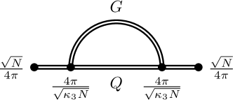
Figure 2.1: The tree-level (top) and one-loop contribution (bottom) to the two-point function of the fermionic operators in the large $N$ limit.

Now the coupling (2.9) can be used to estimate the size of the one-loop gluon partner contribution to the two-point functions relative to that of the tree-level contribution:

$$\frac{\mbox{one-loop}}{\mbox{tree}}=\frac{(N/16\pi^{2})\times(16\pi^{2}/\kappa_{3}N)\times(C_{2}(N_{c})/16\pi^{2})}{(N/16\pi^{2})}\approx\frac{1}{\pi}.$$ (2.10)

The expression on the left hand side is obtained using the large $N$ result $\langle\mathcal{O}_{L}\mathcal{O}_{R}\rangle\sim N/16\pi^{2}$ for the tree-level contribution in the denominator (the top diagram in figure 2.1). For the one-loop gluon partner contribution in the numerator (the bottom diagram in figure 2.1) there are two vertices coupling top partners to a gluon partner, each contributing a factor of $4\pi/\sqrt{\kappa_{3}N}$, an additional loop factor $1/16\pi^{2}$, as well as the quadratic Casimir $C_{2}(3)=4/3$ (coming from $t^{a}t^{a}=C_{2}(N_{c})\mbox{1 \kern-5.89996pt{\rm l}}$, where $t^{a}$ are the generators of $SU(3)$ in the fundamental representation). Finally, we substitute in the estimated value for $\kappa_{3}$ from eq. (2.8) to get a numerical value.

Despite being a higher order effect, we find that the contribution due to the gluon partners could be of order $30\%$. An alternative derivation, based on the mixing between the holographic and mass bases and yielding the same result, is presented in the appendix. Note that these estimates neglect a momentum dependent loop function, which will be explicitly computed in the next section.

2.2 Exact calculation

Figure 2.2: The one-loop contribution to the self energy of a fermion resonance $Q$ from a gluon partner $G$.

To fully quantify the effect of gluon partners on the Higgs mass we must calculate the contribution from figure 2.2 explicitly. This assumes that the gluon partners associated with the current ${\cal J}$ can be modelled as narrow resonances, like their fermionic brethren. Each top partner propagator is renormalised to

$$S^{-1}(p)=S^{-1}_{0}(p)+i\Sigma_{1}(p),$$ (2.11)

at one-loop order, where $S^{-1}_{0}(p)=-i(\not{p}-m_{Q})$ is the unrenormalised propagator and $\Sigma_{1}(p)$ is the one-loop renormalised self energy. Including appropriate counterterms for the wave function and mass renormalisation, this self energy is given by

$$\Sigma_{1}(p)=\Sigma(p)-(\not{p}-m_{Q})\delta Z_{2}-\delta m_{Q},$$ (2.12)

where

$$i\Sigma(p)=\frac{16\pi}{3}\alpha_{G}\int\frac{{\rm d}^{4}k}{(2\pi)^{4}}\,\gamma^{\mu}\frac{1}{\not{k}-m_{Q}}\gamma^{\nu}\frac{\eta_{\mu\nu}}{(k-p)^{2}-m_{G}^{2}},$$ (2.13)

is the integral expression obtained from the diagram in figure 2.2.

Renormalising the propagator in the on-shell scheme gives the two renormalisation conditions

$$\left.\Sigma_{1}(p)\right|_{\not{p}=m_{Q}} =0, \left.\frac{\partial\Sigma_{1}(p)}{\partial\not{p}}\right|_{\not{p}=m_{Q}} =0,$$ (2.14)

which are used to determine the two counter terms $\delta Z_{2}$ and $\delta m_{Q}$. By writing

$$\Sigma(p)=m_{Q}A(p^{2})+\not{p}B(p^{2}),$$ (2.15)

then solving the above equations and substituting into eqs. (2.11) and (2.12), we find the one-loop expression

$$iS^{-1}(p)=\left(1-\widehat{B}(p^{2})+\left.m_{Q}\frac{\partial}{\partial\not{p}}\left[\widehat{A}(p^{2})+\widehat{B}(p^{2})\right]\right|_{\not{p}=m_{Q}}\right)\left(\not{p}-m_{Q}\left[1+\widehat{A}(p^{2})+\widehat{B}(p^{2})\right]\right),$$ (2.16)

where we have further defined

$$\widehat{A}(p^{2}) =A(p^{2})-A(m_{Q}^{2}), \widehat{B}(p^{2}) =B(p^{2})-B(m_{Q}^{2}).$$ (2.17)

The first factor in (2.16) is absorbed into an overall rescaling of the top partner fields and is not important for our purposes. The second term can be expressed in the propagator as an effective correction to the top partner mass

$$\Delta m_{Q}(p^{2})=m_{Q}\left[\widehat{A}(p^{2})+\widehat{B}(p^{2})\right].$$ (2.18)

We now need to evaluate eq. (2.13) to determine the functions $\widehat{A}(p^{2})$ and $\widehat{B}(p^{2})$. The answer is succinctly expressed in terms of Passarino-Veltman integrals [23] (see the appendix)

$$i\Sigma(p) =\frac{2\alpha_{G}}{3\pi^{3}}\int{\rm d}^{4}k\,\frac{2m_{Q}-\not{k}}{[k^{2}-m_{Q}^{2}][(k-p)^{2}-m_{G}^{2}]}$$

$$=\frac{2i\alpha_{G}}{3\pi}\left[2m_{Q}B_{0}(p^{2},m_{Q}^{2},m_{G}^{2})+\not{p}B_{1}(p^{2},m_{Q}^{2},m_{G}^{2})\right],$$ (2.19)

and therefore

$$\widehat{A}(p^{2}) =\frac{4\alpha_{G}}{3\pi}\left[B_{0}(p^{2},m_{Q}^{2},m_{G}^{2})-B_{0}(m_{Q}^{2},m_{Q}^{2},m_{G}^{2})\right],$$ (2.20)

$$\widehat{B}(p^{2}) =\frac{2\alpha_{G}}{3\pi}\left[B_{1}(p^{2},m_{Q}^{2},m_{G}^{2})-B_{1}(m_{Q}^{2},m_{Q}^{2},m_{G}^{2})\right].$$ (2.21)

In an explicit integral form we find the final result

$$\Delta m_{Q}(p^{2})=\frac{2\alpha_{G}}{3\pi}m_{Q}\int_{0}^{1}\mathrm{d}x\,(x-2)\ln\left[\frac{(1-x)m_{Q}^{2}+xm_{G}^{2}-x(1-x)p^{2}}{(1-x)^{2}m_{Q}^{2}+xm_{G}^{2}}\right].$$ (2.22)

This one-loop result can be easily generalised to include contributions from multiple gluon partners by replacing the above expression (2.22) with a sum of identical terms, each using different values for $\alpha_{G}$ and $m_{G}$. However, we expect that the lightest gluon partner will always dominate because the loop integral can be seen to decrease as the gluon partner mass is increased, and the coupling is expected to behave similarly (this latter effect can be seen explicitly in the 5D calculation).

2.3 Electroweak and other contributions

In addition to the coloured contribution we can estimate the equivalent non-coloured contribution arising from the electroweak resonances. Using the relation (2.7) we obtain

$$\frac{1}{N}=\frac{g_{2}^{2}}{16\pi^{2}}\ln\left(\frac{\Lambda_{\rm UV}}{\Lambda_{\rm IR}}\right)\approx\frac{1}{4\pi},$$ (2.23)

where $\alpha_{2}\approx 1/30$ is the electroweak coupling strength and, for simplicity, we have set $\kappa_{2}=1$, corresponding to a redefinition of $N$. This enables us to estimate the coupling $\alpha_{\rho}$ of the top partner fermions with the electroweak vector mesons. Using eq. (2.23) we obtain $\alpha_{\rho}=4\pi/N=1$. This is a factor of three smaller than the gluon coupling (2.9). The ratio of the electroweak resonance correction relative to that of the gluon partner correction is then $[\alpha_{\rho}C_{2}(2)]/[\alpha_{G}C_{2}(3)]\simeq 3/16$, where we have further used the $SU(2)$ quadratic Casimir $C_{2}(2)=3/4$. Thus the correction coming from electroweak vector mesons is much less important than the gluon partner correction, and will henceforth be neglected.

Having gone beyond leading order in $1/N$ one may anticipate that other corrections to the Higgs potential, beyond the simple mass shift of eq. (2.22), should be considered. While such corrections do exist, and are at the same order in $1/N$, they will always be subdominant. The reason is that the correction calculated above is the only one proportional to the top partner-gluon partner coupling $\alpha_{G}$, in contrast to other corrections which go like $\sqrt{\alpha_{G}\alpha_{3}}$ or just $\alpha_{3}$. The couplings in the coloured sector satisfy $\alpha_{G}\gg\alpha_{3}$, as shown in the previous subsection, hence any other corrections coming from this sector can be neglected. The situation is even more acute in the non-coloured sector, as these corrections suffer a similar suppression from the reduced coupling strength, and do not even benefit from QCD multiplicity factors when evaluating loops. Another correction one might consider beyond leading order in $1/N$ is a wave function renormalisation of the Higgs. However, in this framework the Higgs always appears in the ratio $h/f$, meaning that any wave function renormalisation is simply absorbed in a rescaling of the symmetry breaking scale.

While the above arguments are robust in the models we are considering here, where the strong sector only communicates with elementary fields through bilinear couplings like those in eq. (2.1), they do not immediately apply in more general models. Then, there may be other corrections to the Higgs mass of similar importance. However, it should be noted that the effective Lagrangian (2) will no longer apply either. Such models are beyond the scope of this paper, but could result in interesting deviations from the usual behaviour found in composite Higgs models.

3 Effect on the minimal composite Higgs mass

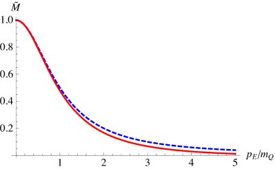
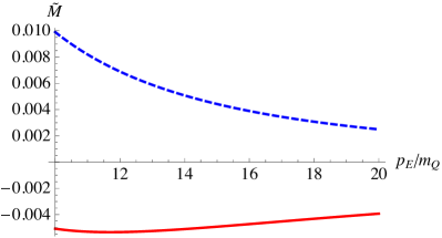
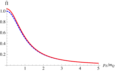
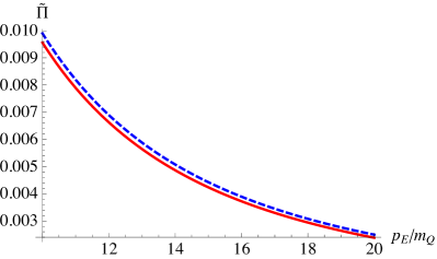
Figure 3.1: The effect of the gluon partner correction on the normalised form factors $\widetilde{M}(p_{E}^{2})\equiv v/(\sqrt{2}fm_{t})M(p_{E}^{2})$ (top) and $\widetilde{\Pi}(p_{E}^{2})\equiv(m_{Q}/M(0))\Pi(p_{E}^{2})$ (bottom). The functions are evaluated using eq. (3) for a single top and gluon partner resonance, fixing $a=b=1$ and $F_{L}=F_{R}$ for simplicity. The normalisation is chosen to respect the top mass constraint in eq. (3.6). The dashed lines show the uncorrected functions and the solid lines show the effect of gluon partner correction for $\alpha_{G}=3$ and $m_{G}=3$ TeV.

The leading order effect of gluon partners on the Higgs mass in the large $N$ limit is accounted for by shifting the mass parameters in eq. (2.4) using the expression in eq. (2.22). One then uses the renormalised functions

$$M(p^{2}) =\sum_{n=1}^{\infty}\frac{b_{n}F^{L}_{n}F^{R}_{n}{}^{*}(m_{Q_{n}}+\Delta m_{Q_{n}}(p^{2}))}{p^{2}-(m_{Q_{n}}+\Delta m_{Q_{n}}(p^{2}))^{2}},$$

$$\Pi(p^{2})_{L/R} =\sum_{n=1}^{\infty}\frac{a_{n}|F^{L/R}_{n}|^{2}}{p^{2}-(m_{Q_{n}}+\Delta m_{Q_{n}}(p^{2}))^{2}},$$ (3.1)

to calculate the Higgs potential in eq. (2). Leaving these functions as they are, i.e. not expanding in $\alpha_{G}$ again, ensures that the approximation remains good at high momentum, and corresponds to consistently resumming all contributions generated by the 1PI diagram in figure 2.2. This is easily seen to be the leading order effect. Note also that, since the correction shows up as a mass shift only, all of the group structure is preserved and we can simply apply existing results to calculate the Higgs mass with no need to worry about the theory becoming non-renormalisable. This may not have been the case if the renormalisation procedure had introduced momentum dependence into the $F$’s.

To get an idea how the form factors are changed, we evaluate eq. (3) with a single top partner, a single gluon partner, and with all unknown constants fixed using a normalisation respecting eq. (3.6). This results in form factors behaving as in figure 3.1. The corrected form factor $M(p_{E})$ (that provides the top quark Yukawa) is seen to decrease relative to the uncorrected form factor at low momentum, but it then crosses zero and continues to decrease to a magnitude bigger than the uncorrected function. This does not imply that the one-loop result has become unreliable, as the expansion parameter when renormalising the propagator goes like $\Delta m_{Q}/(\not{p}_{E}+m_{Q})$, which is still much less than one at large momentum. Meanwhile the corrected form factor $\Pi(p_{E})$ displays the opposite behaviour; it is seen to increase relative to the uncorrected form factor at low momentum, but it decays more quickly so ends up smaller than the uncorrected function at high momentum.

The way that these form factors appear in the Higgs potential (2) is model dependent so we cannot make a universal statement about how the gluon partner correction changes the Higgs mass. Even for a specific model it is not obvious what will happen. Only the magnitude of $M(p_{E})$ appears in eq. (2), so there is always some cancellation when performing the momentum integral and it is not immediately apparent whether the Higgs mass will be increased or decreased. A similar cancellation occurs when integrating $\Pi(p_{E})$, and the situation is further complicated by including more top parters, whereupon there can be cancellations in the expressions (3) even before integrating over momentum. Nonetheless, eqs. (2.22) and (3) are all that is needed to calculate the leading order gluon partner correction to the Higgs mass in any model of this form.

As a specific example we now consider the minimal composite Higgs model (MCHM). This is based on the symmetry breaking pattern $SO(5)\to SO(4)$ and supports numerous embeddings for the top quarks. If the left handed doublet and right handed singlet are both embedded into ${\bf 5}$’s (the MCHM₅) the Higgs mass is given by [10, 11]

$$m_{h}^{2}\approx\frac{8N_{c}v^{2}}{f^{4}}\int\frac{\mathrm{d}^{4}p_{E}}{(2\pi)^{4}}\,\left[\frac{\left|M(p_{E}^{2})\right|^{2}}{p_{E}^{2}\Pi_{L}^{0}(p_{E}^{2})\Pi_{R}^{0}(p_{E}^{2})}+\left(\frac{\Pi_{L}^{h}(p_{E}^{2})}{2\Pi^{0}_{L}(p_{E}^{2})}\right)^{2}+\left(\frac{\Pi_{R}^{h}(p_{E}^{2})}{\Pi^{0}_{R}(p_{E}^{2})}\right)^{2}\right],$$ (3.2)

where $N_{c}=3$ and $v=246$ GeV is the Higgs VEV. This expression simplifies when the mixing between elementary and composite degrees of freedom is small, such that $\Pi_{L/R}^{0}\approx 1$ (equivalently $|F|\ll m_{Q}$), to become

$$m_{h}^{2}\approx\frac{8N_{c}v^{2}}{f^{4}}\int\frac{\mathrm{d}^{4}p_{E}}{(2\pi)^{4}}\,\left[\frac{1}{p_{E}^{2}}\left|M(p_{E}^{2})\right|^{2}+\frac{1}{4}\Pi_{L}^{h}(p_{E}^{2})^{2}+\Pi_{R}^{h}(p_{E}^{2})^{2}\right].$$ (3.3)

Using Weinberg sum rules [25] refs. [10, 11] show that at least two top partners are required for the Higgs potential to be convergent in this model. For concreteness we will consider only two low mass states. Denoting their masses by $m_{Q_{1}}$ and $m_{Q_{4}}$ (corresponding to their $SO(4)$ representations) the uncorrected functions in eq. (2.4) then take the specific forms

$$\Pi^{h(0)}_{L/R}(p^{2}) =|F^{L/R}|^{2}\frac{m_{Q_{4}}^{2}-m_{Q_{1}}^{2}}{(p^{2}-m_{Q_{4}}^{2})(p^{2}-m_{Q_{1}}^{2})},$$

$$M^{(0)}(p^{2}) =|F^{L}F^{R}|\frac{m_{Q_{4}}m_{Q_{1}}(m_{Q_{4}}-m_{Q_{1}}e^{i\theta})}{(p^{2}-m_{Q_{4}}^{2})(p^{2}-m_{Q_{1}}^{2})}\left[1-\frac{p^{2}}{m_{Q_{4}}m_{Q_{1}}}\frac{m_{Q_{1}}-m_{Q_{4}}e^{i\theta}}{m_{Q_{4}}-m_{Q_{1}}e^{i\theta}}\right],$$ (3.4)

where $\theta$ is the phase difference between form factors, i.e. $F^{L}F^{R}{}^{*}=e^{i\theta}|F^{L}F^{R}|$ and the subscripts have been omitted from the $F^{L/R}$ (which have been set to be equal by a field redefinition).

Substituting into eq. (3.3) and integrating, one arrives at the uncorrected expression

$$[m_{h}^{2}]^{(0)}\approx\frac{N_{c}}{\pi^{2}}\frac{m_{t}^{2}}{f^{2}}\frac{m_{Q_{4}}^{2}m_{Q_{1}}^{2}}{m_{Q_{4}}^{2}-m_{Q_{1}}^{2}}\ln\left(\frac{m_{Q_{4}}^{2}}{m_{Q_{1}}^{2}}\right).$$ (3.5)

To eliminate both form factors and the phase $\theta$ from the above expression two relationships have been used, which will continue to be assumed throughout the rest of this paper. First one takes $\Delta F^{2}=|F^{L}|^{2}-2|F^{R}|^{2}=0$. This is helpful in arranging for electroweak symmetry breaking, as there is an additional, positive contribution to the quadratic term in the potential proportional to $\Delta F^{4}$. Then one uses the expression for the top mass

$$m_{t}^{2}\approx\frac{v^{2}}{2f^{2}}|M(0)|^{2},$$ (3.6)

which follows from reading off the Yukawa coupling from the effective Lagrangian (2) in the low energy limit $p^{2}\approx 0$.

If the renormalised expressions (3) are substituted into eq. (3.3) there is no simple analytic expression for the functions $\Pi$ and $M$. Nonetheless, we can still apply the two relationships used above to solve for the $F$’s, upon which the integrals can all be performed and the effect of the gluon partner quantified.

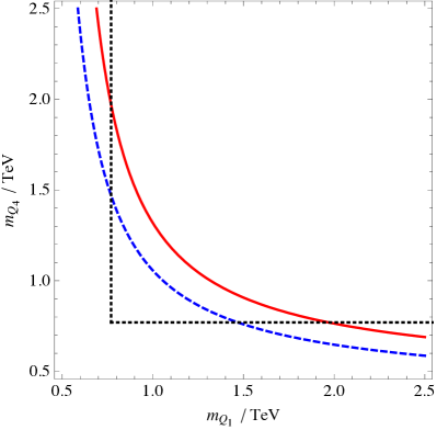
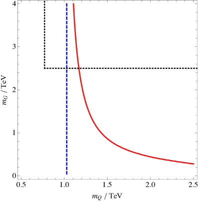
Figure 3.2: Contours of $m_{h}=126$ GeV for $\alpha_{G}=3$, $v^{2}=0.1f^{2}$ and $m_{t}=173$ GeV. Blue, dashed lines represent the result without massive gluons from ref. [11] and solid, red lines the result including gluon partners calculated here. Black dotted lines represent approximate experimental limits for the top partners and gluon partners of 770 GeV [27] and 2.5 TeV [26] respectively. Left: Two different mass top partners with a 3 TeV gluon partner. Right: Two equal mass top partners with variable gluon partner mass.

In figure 3.2 we show contours of $m_{h}=126$ GeV in the $(m_{Q_{1}},m_{Q_{4}})$ plane for two distinct top partner masses. Both the uncorrected result from ref. [11] (blue, dashed) and our result, that includes the gluon partner correction (red, solid), is shown. For distinct top partner masses the phase $\theta$ can no longer be completely absorbed because the top mass is evaluated at a fixed momentum but the gluon partner correction, which changes the phase dependence, varies with momentum. However, we have checked that the $\theta$ dependence is only mild, so we fix $\cos{\theta}=-1$ for definiteness. In addition, we include approximate experimental limits for the top partners (770 GeV [27]) and gluon partners (2.5 TeV [26]).

The main message of figure 3.2 is that the top partner masses that result in $m_{h}=126$ GeV are universally shifted to larger values. The shift is significant, as predicted by the discussion in section 2.1, and provides additional breathing space for the model with respect to collider searches.

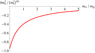
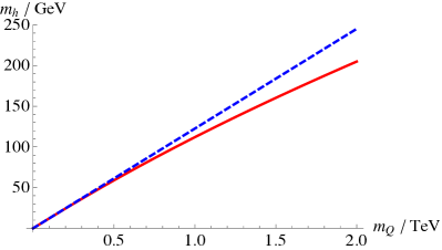
Figure 3.3: Left: The ratio of the correction $\delta m_{h}^{2}=([m_{h}^{2}]^{(1)}-[m_{h}^{2}]^{(0)})$ to the uncorrected Higgs mass squared as a function of $m_{G}/m_{Q}$ for two equal mass top partners. Right: The absolute Higgs mass as a function of $m_{Q}$ with $m_{G}=3$ TeV in the same scenario. The dashed line represents the result without massive gluons from ref. [11] and the solid line the result including gluon partners calculated here. In both plots $\alpha_{G}=3$, $v^{2}=0.1f^{2}$ and $m_{t}=173$ GeV.

It is also instructive to consider the special case in which the two resonances are degenerate in mass: $m_{Q_{4}}=m_{Q_{1}}\equiv m_{Q}$. This gives an uncorrected Higgs mass value of $[m_{h}^{2}]^{(0)}=N_{c}m_{t}^{2}m_{Q}^{2}/\pi^{2}f^{2}$. In figure 3.2 and 3.3 we show the effect of the gluon partner correction in this scenario. On the left of figure 3.3 is the size of the gluon partner correction relative to the uncorrected result. The correction is always negative (i.e. the Higgs mass is decreased) and decreases in magnitude as the ratio $m_{G}/m_{Q}$ is increased and the gluon partner decouples. On the right of figure 3.3 is the absolute Higgs mass as a function of $m_{Q}$ for $m_{G}=3$ TeV, explicitly showing the reduction of the Higgs mass relative to the uncorrected result. The change in the value of the top partner mass required for a 126 GeV Higgs can be found more precisely in this case; it is increased from 1 TeV to 1.1 TeV – a relative change of 10%.

4 Conclusion

Gluon partners are generically present in composite Higgs models that include top partners in their low energy spectrum. The gluon partners are expected to couple strongly to the top partners, and this expectation is quantitatively confirmed by arguments based on holography. They can therefore provide a significant correction to the composite Higgs mass. The leading order correction is parameterised by a momentum dependent top partner mass shift in the two-point functions of the strong sector, which we have explicitly calculated in this paper. The final effect on the Higgs mass is model dependent, but we find a decrease in the Higgs mass in the MCHM₅. This means that the mass of the top partners required to yield a 126 GeV Higgs is increased by about 10% (for a 3 TeV gluon partner and a spontaneous global symmetry breaking scale of about 750 GeV) easing constraints from direct collider searches for top partners.

Appendix A Holographic basis estimate

We can also use the mixing between the holographic and mass bases to estimate the size of the one-loop correction resulting from massive gluons. At next to leading order in $1/N$ there are gluon partner contributions to the two-point functions of ${\cal O}_{L}$ and ${\cal O}_{R}$. For simplicity, let us assume that the strong sector only produces one gluon partner, $G_{c}$, that mixes with the elementary gluon, $A_{e}$, so that the mass eigenstates can be written as

$$A_{g}^{\mu} =A^{\mu}_{e}\cos{\theta}+G_{c}^{\mu}\sin{\theta}, G^{\mu} =G_{c}^{\mu}\cos{\theta}-A^{\mu}_{e}\sin{\theta},$$ (A.1)

where $A_{g}$ is the (massless) physical gluon and $G$ is the massive gluon. There is then one diagram for each mass eigenstate propagating around the loop. Each diagram gets a factor of $\alpha_{G}$ from the $\bar{Q}\not{G}_{c}Q$ coupling in the strong sector, and a $\sin^{2}\theta$ or $\cos^{2}\theta$ from the $G_{c}$-$A_{e}$ mixing to give

$$\Sigma_{g} \sim\frac{N\alpha_{G}}{(4\pi)^{3}}\sin^{2}\theta\,C_{2}(N_{c}), \Sigma_{G} \sim\frac{N\alpha_{G}}{(4\pi)^{3}}\cos^{2}\theta\,C_{2}(N_{c}),$$ (A.2)

where $C_{2}(3)=4/3$ is the quadratic Casimir for the fundamental representation of $SU(3)$ and $\Sigma_{g,G}$ is multiplied by an order one loop function. The factor of $N$ comes from factors of $\sqrt{N}/(4\pi)$ on each external leg, themselves originating from vacuum creation amplitudes. Although $\alpha_{G}$ scales like $1/N$ it can still be large if this scaling comes with a large prefactor.

In the case at hand we know from gauge invariance that $\alpha_{G}\sin^{2}\theta=\alpha_{3}$. We also know from holographic arguments that $\sin^{2}\theta\approx 1/\pi kR\approx 1/30$ (see e.g. ref. [28] or ref. [19] for an explicit calculation). Hence $\alpha_{G}\approx 30\alpha_{3}$, clearly overcoming any $1/N$ suppression, and we find

$$\Sigma_{G}\sim\frac{10N\alpha_{3}}{16\pi^{3}}.$$ (A.3)

The ratio of the one-loop result with the tree-level result $\sim N/(16\pi^{2})$ gives a factor $1/\pi$ , which is the same as obtained in section 2.1.

Appendix B Passarino-Veltman integrals

Expressions for the Passarino-Veltman integrals used are

$$B_{0}(p^{2},m_{Q}^{2},m_{G}^{2}) =\frac{1}{i\pi^{2}}\int\mathrm{d}^{4}k\,\frac{1}{[k^{2}-m_{Q}^{2}][(k-p)^{2}-m_{G}^{2}]}$$

$$=\Delta_{\epsilon}-\int_{0}^{1}\mathrm{d}x\,\ln\left[\frac{xm_{G}^{2}+(1-x)m_{Q}^{2}-x(1-x)p^{2}}{\mu^{2}}\right],$$ (B.1)

$$B^{\mu}(p^{2},m_{Q}^{2},m_{G}^{2}) =\frac{1}{i\pi^{2}}\int\mathrm{d}^{4}k\,\frac{k^{\mu}}{[k^{2}-m_{Q}^{2}][(k-p)^{2}-m_{G}^{2}]}$$

$$=p^{\mu}B_{1}(p^{2},m_{Q}^{2},m_{G}^{2})$$

$$=p^{\mu}\left(-\frac{1}{2}\Delta_{\epsilon}+\int_{0}^{1}\mathrm{d}x\,x\ln\left[\frac{xm_{G}^{2}+(1-x)m_{Q}^{2}-x(1-x)p^{2}}{\mu^{2}}\right]\right),$$ (B.2)

where $\mu$ is the renormalisation scale.

References

- [1] CMS Collaboration, S. Chatrchyan et. al., Observation of a new boson at a mass of 125 GeV with the CMS experiment at the LHC, Phys.Lett. B716 (2012) 30–61 [1207.7235].
- [2] CMS Collaboration, S. Chatrchyan et. al., Observation of a new boson with mass near 125 GeV in collisions at and 8 TeV, 1303.4571.
- [3] ATLAS Collaboration, G. Aad et. al., Observation of a new particle in the search for the Standard Model Higgs boson with the ATLAS detector at the LHC, Phys.Lett. B716 (2012) 1–29 [1207.7214].
- [4] S. P. Martin, A supersymmetry primer, hep-ph/9709356.
- [5] D. B. Kaplan and H. Georgi, Breaking by Vacuum Misalignment, Phys.Lett. B136 (1984) 183.
- [6] H. Georgi and D. B. Kaplan, Composite Higgs and Custodial , Phys.Lett. B145 (1984) 216.
- [7] T. Gherghetta, B. von Harling, A. D. Medina and M. A. Schmidt, The Scale-Invariant NMSSM and the 126 GeV Higgs Boson, JHEP 1302 (2013) 032 [1212.5243].
- [8] R. Contino, Y. Nomura and A. Pomarol, Higgs as a holographic pseudo-Goldstone boson, Nucl.Phys. B671 (2003) 148–174 [hep-ph/0306259].
- [9] O. Matsedonskyi, G. Panico and A. Wulzer, Light Top Partners for a Light Composite Higgs, JHEP 1301 (2013) 164 [1204.6333].
- [10] D. Marzocca, M. Serone and J. Shu, General Composite Higgs Models, JHEP 1208 (2012) 013 [1205.0770].
- [11] A. Pomarol and F. Riva, The Composite Higgs and Light Resonance Connection, JHEP 1208 (2012) 135 [1205.6434].
- [12] G. Panico, M. Redi, A. Tesi and A. Wulzer, On the Tuning and the Mass of the Composite Higgs, JHEP 1303 (2013) 051 [1210.7114].
- [13] D. Pappadopulo, A. Thamm and R. Torre, A minimally tuned composite Higgs model from an extra dimension, JHEP 1307 (2013) 058 [1303.3062].
- [14] K. Agashe, R. Contino and A. Pomarol, The minimal composite Higgs model, Nucl.Phys. B719 (2005) 165–187 [hep-ph/0412089].
- [15] A. D. Medina, N. R. Shah and C. E. Wagner, Gauge-Higgs Unification and Radiative Electroweak Symmetry Breaking in Warped Extra Dimensions, Phys.Rev. D76 (2007) 095010 [0706.1281].
- [16] B. Gripaios, A. Pomarol, F. Riva and J. Serra, Beyond the Minimal Composite Higgs Model, JHEP 0904 (2009) 070 [0902.1483].
- [17] J. Mrazek, A. Pomarol, R. Rattazzi, M. Redi, J. Serra et. al., The Other Natural Two Higgs Doublet Model, Nucl.Phys. B853 (2011) 1–48 [1105.5403].
- [18] E. Bertuzzo, T. S. Ray, H. de Sandes and C. A. Savoy, On Composite Two Higgs Doublet Models, JHEP 1305 (2013) 153 [1206.2623].
- [19] M. Carena, A. D. Medina, B. Panes, N. R. Shah and C. E. Wagner, Collider phenomenology of gauge-Higgs unification scenarios in warped extra dimensions, Phys.Rev. D77 (2008) 076003 [0712.0095].
- [20] T. Gherghetta and A. Pomarol, A Distorted MSSM Higgs Sector from Low-Scale Strong Dynamics, JHEP 1112 (2011) 069 [1107.4697].
- [21] C. Csaki, A. Falkowski and A. Weiler, The Flavor of the Composite Pseudo-Goldstone Higgs, JHEP 0809 (2008) 008 [0804.1954].
- [22] K. Agashe, A. Azatov and L. Zhu, Flavor Violation Tests of Warped/Composite SM in the Two-Site Approach, Phys.Rev. D79 (2009) 056006 [0810.1016].
- [23] G. Passarino and M. Veltman, One Loop Corrections for Annihilation Into in the Weinberg Model, Nucl.Phys. B160 (1979) 151.
- [24] B. Bellazzini, C. Csaki, J. Hubisz, J. Serra and J. Terning, Composite Higgs Sketch, JHEP 1211 (2012) 003 [1205.4032].
- [25] S. Weinberg, Precise relations between the spectra of vector and axial vector mesons, Phys.Rev.Lett. 18 (1967) 507–509.
- [26] Search for resonances in semileptonic final state, Tech. Rep. CMS-PAS-B2G-12-006, CERN, Geneva, Apr, 2013.
- [27] Search for top partners in same-sign dilepton final state, Tech. Rep. CMS-PAS-B2G-12-012, CERN, Geneva, Mar, 2013.
- [28] T. Gherghetta, TASI Lectures on a Holographic View of Beyond the Standard Model Physics, 1008.2570.