Abstract

In currently most popular explicitly correlated electronic structure theories the dependence of the wave function on the interelectronic distance $r_{ij}$ is built via the correlation factor $f(r_{ij})$. While the short-distance behavior of this factor is well understood, little is known about the form of $f(r_{ij})$ at large $r_{ij}$. In this work we investigate the optimal form of $f(r_{12})$ on the example of the helium atom and helium-like ions and several well-motivated models of the wave function. Using the Rayleigh-Ritz variational principle we derive a differential equation for $f(r_{12})$ and solve it using numerical propagation or analytic asymptotic expansion techniques. We found that for every model under consideration, $f(r_{12})$ behaves at large $r_{ij}$ as $r_{12}^{\rho}\,e^{Br_{12}}$ and obtained simple analytic expressions for the system dependent values of $\rho$ and $B$. For the ground state of the helium-like ions the value of $B$ is positive, so that $f(r_{12})$ diverges as $r_{12}$ tends to infinity. The numerical propagation confirms this result. When the Hartree-Fock orbitals, multiplied by the correlation factor, are expanded in terms of Slater functions $r^{n}e^{-\beta r}$, $n=1\ldots N$, the numerical propagation reveals a minimum in $f(r_{12})$ with depth increasing with $N$. For the lowest triplet state $B$ is negative. Employing our analytical findings, we propose a new “range-separated” form of the correlation factor with the short- and long-range $r_{12}$ regimes approximated by appropriate asymptotic formulas connected by a switching function. Exemplary calculations show that this new form of $f(r_{12})$ performs somewhat better than the correlation factors used thus far in the standard R12 or F12 theories.

^ae-mail: lesiuk@tiger.chem.uw.edu.pl

I Introduction

It is well known that the slow convergence of the standard, orbital based methods of the electronic structure theory is due to the difficulties to model the exact wave function in the regions of the configurations space where electrons are close to each otherhattig12 ; kong12 . It was shown by Katokato57 and later elaborated by Pack and Byers-Brownpack66 , and Hoffman-Ostenhofs et al.furnais05 ; hoffmann92 that in the vicinity of points where the positions of two electrons coincide, the wave function behaves linearly in the interelectronic distance $r_{12}$. Such a behavior, referred often to as the cusp condition, cannot be modeled by a finite expansion in terms of orbital productsszalewicz10 . The solution to this problem is to include the interelectronic distance dependence directly into the wave function. This is the main idea of the so-called explicitly correlated methods of the electronic structure theoryhattig12 ; kong12 ; tenno12 . It should be noted however, that the explicit dependence on $r_{12}$ is advantageous even if the cusp condition is not fulfilled exactly as in the Gaussian geminalszalewicz10 ; bukowski03 or the ECGrychlewski03 ; bubin13 (explicitly correlated Gaussian) approaches. This is due to the fact that the correlation hole, i.e., the decrease of the wave function amplitude when the electrons approach each other, is much easier to model with basis functions depending explicitly on $r_{12}$ than with the orbital productsszalewicz10 .

The simplest way to make the wave function $r_{12}$ dependent is to multiply some or all orbital products in its conventional configuration-interaction-type expansion by a correlation factor $f(r_{12})$. In this way all $r_{12}$ dependence is contracted in one function of single variable. The idea of the correlation factor is very old one. It can be traced back to the late 1920’s work of Slaterslater28 and of Hylleraashylleraas29a ; hylleraas29b who showed great effectiveness of including the linear $r_{12}$ term in the helium wave function. More than two decades later Jastrowjastrow55 proposed to use the correlation factor to construct a compact form of correlated wave function for an N-particle quantum system. The wave function form proposed by Jastrow became popular in the electronic structure theory as the guide function in diffusion-equation Monte-Carlo calculationsluchow00 ; foulkes01 .

The concept of the correlation factor is now most widely used in the context of many-body perturbation theorykucharski86 (MBPT) and coupled clusterbartlett07 (CC) approach. It was first observed by Byron and Joachainbyron66 , and later by Pan and Kingpan70 ; pan72 , Szalewicz and co-workers,chalas77 ; szalewicz79 ; szalewicz82 ; szalewicz83b ; szalewicz84 , and Adamowicz and Sadlejadamowicz77 ; adamowicz78a ; adamowicz78b that the pair functions appearing in the energy expressions of the MBPT or CC theory can be very efficiently approximated when expanded in terms of explicitly correlated basis functions. In the investigations of Refs. pan70 –adamowicz78b the dependence on the $r_{12}$ coordinate was introduced through the Gaussian factors, $\exp{(-\gamma_{i}r^{2}_{12})}$, with different $\gamma_{i}$ for different basis functions (Gaussian geminals). Thus, the pair functions were not represented with a single, universal correlation factor. Massive optimizations of thousands of nonlinear parameters defining the Gaussian geminals ($\gamma_{i}$ and orbital exponents) made these calculations very time-consuming, limiting applications of this approach to very small systems like Be, Li^-, LiH, He₂, Ne, or H₂Obukowski99 ; przybytek09 ; patkowski07 ; wenzel86 ; bukowski95 .

An important advance in the field of explicitly correlated MBPT/CC theory came with the seminal 1985 work of Kutzelniggkutz85 and the subsequent development of the so-called R12 method by Kutzelnigg, Klopper and Nogaklopper87 ; kutz91 ; noga92 ; noga94 ; klopper03 . In this work a simple linear correlation factor $f(r_{12})=r_{12}$ was used to multiply products of occupied Hartree-Fock (HF) orbitals $\phi_{i}$, $i=1,\ldots n$. The resulting set of explicitly correlated basis functions $f(r_{12})\phi_{i}\phi_{j}$, supplemented by products of all virtual orbitals, was then used to expand the pair functions of the MBPT/CC theory. The necessity to calculate three and four-electron integrals, resulting from the Coulomb and exchange operators and the strong orthogonality projectors, is eliminated by suitable resolution of identity (RI) insertions. Kutzelnigg and Klopper introduced also some useful approximationsklopper87 ; kutz91 to the expression for the commutator of the Fock operator with $f(r_{12})$ which significantly simplified calculations. The practical implementation of the original R12 scheme was, however, not free from problems. Most importantly, in order to make the RI approximation accurate enough the one-electron basis set used in calculations had to be very large. This constraint was alleviated by Klopper and Samsonklopper02 who introduced auxiliary basis sets for the RI approximation which are saturated independently from the size of the basis set that is used in the preceding Hartree-Fock calculations. During the past two decades the R12 technology was progressively refined by the use of many tricks such as the density fittingmanby03 , numerical quadraturestenno04a , improvements in the RI approximationstenno03 ; valeev04a , or efficient parallel implementations.valeev00 ; valeev04b A generalizations to multi-reference configuration interaction problems (MRCI-R12) have been developed by Gdanitzgdanitz93 ; gdanitz98 . One should also mention the work of Taylor and co-workerspersson96 ; persson97 ; dahle01 who expanded the linear correlation factor $r_{12}$ as a combination of the Gaussian functions, and evaluated the necessary many-electron integrals analytically.

Despite this progress, the results of R12 calculations using small basis sets were l not fully satisfying. In particular, it was shown that the results of R12 calculations with a correlation-consistent polarized valence double-zeta (cc-pVDZ) basis set were of similar quality as ordinary orbital based calculations with a triple-zeta cc-pVTZ basis setklopper02 . This is a rather small gain when compared to the accuracy improvement in calculations with the quintuple-zeta basis sets when the R12 method gives almost saturated results. In 2005 May and co-workersmay05 reported a careful analysis of the errors in R12 theory at the second-order Møller-Plesset (MP2-R12) level. They concluded that the most significant source of these errors are defects inherent in the R12 Ansatz and that it is essential that $r_{12}$ is replaced by a more accurate correlation factor $f(r_{12})$. Actually, a generalization of the R12 theory, referred to as the F12 theory, allowing an arbitrary, nonlinear correlation factor $f(r_{12})$ was formulated by May and Manbymay04 already in 2004. In the same year Ten-notenno04b proposed the use of the exponential correlation factor $[1-\exp(-\gamma r_{12})]/\gamma$ (Slater-type geminal) and showed that it leads to much better results than the linear one. This launched rapid development of the F12 methods, which are now almost exclusively based on the application of the exponential correlation factor.kong12 ; tenno12 . This correlation factor turned out to be effective not only in the conventional single-reference MBPT/CC theory but was also successfully applied to improve the basis set convergence of multireference methods: MRCIshiozaki11a ; shiozaki11b , multireference perturbation theory torheyden09 ; tenno07 ; shiozaki10 , multireference CC approach kedzuch11 , and even the multiconfiguration SCF proceduremartinez10 .

It is clear that the shape of the correlation factor is important for the high quality of the results. One may, thus, ask what is the optimal form of $f(r_{12})$ that is correct not only in the vicinity of the electrons coalescence points, but also at arbitrary distance between electrons. This question has been considered by Tew and Kloppertew05 who have investigated the shape of the correlation factor for the helium atom and for helium-like ions and compared it with several simple analytic forms. These authors expanded $f(r_{12})$ as a polynomial in $r_{12}$ and determined its coefficients by minimizing the distance (in the Hilbert space) between the exact wave function and its approximate form constructed using $f(r_{12})$. They found that the exponential correlation factor proposed by Ten-notenno04b is close to optimal.

It should be pointed out that the method used by Tew and Kloppertew05 is not accurate at larger values of $r_{12}$ and does not give any information about the asymptotic behavior of $f(r_{12})$ at large $r_{12}$. This is a consequence of the assumed polynomial form for $f(r_{12})$, which prejudges the asymptotic behavior of $f(r_{12})$ and makes the obtained approximation to the optimal $f(r_{12})$ less reliable at larger $r_{12}$. Moreover, the optimum $f(r_{12})$ as defined by Tew and Klopper does not guarantee the minimum energy with respect to a variation of a fully flexible form of the correlation factor.

In the present communication we propose an alternative method to determine the optimal form of $f(r_{12})$, which is free from the above drawbacks. We do not expand $f(r_{12})$ in a basis set but derive a differential equation for $f(r_{12})$, resulting from the unconstrained minimization of the Rayleigh-Ritz energy functional. This differential equation can be solved by a numerical propagation or using analytic, asymptotic expansion techniques. In this way the problems with the stability of the optimal $f(r_{12})$ at large $r_{12}$, experienced by Tew and Kloppertew05 , are avoided and we obtain a reliable information on the large $r_{12}$ behavior of $f(r_{12})$. This information, combined with the well known information about the short-range behavior of $f(r_{12})$, gives us a possibility to propose a new form of the correlation factor which is correct at small and large values of $r_{12}$. One may hope that the correlation factor more adequate at large $r_{12}$ will make up for the lack of flexibility of the orbital basis to describe the long-range correlation and will reduce the basis-set requirements of F12 calculations.

The paper is organized as follows. In Sections II.1 and II.2 we analyze the simplest models of the correlated wave functions for the ground and the lowest triplet state of the helium atom and helium-like ions. In both cases, we establish differential equations for the correlation factor $f(r_{12})$ and solve them exactly in the large-$r_{12}$ domain. In Section II.3 we investigate another model for the singlet ground state when the 1$s$ Slater orbital is replaced by a single Gaussian function. In Section II.4 we move on to the case of a self-consistent-field (SCF) determinant multiplied by the correlation factor. In this case, we were not able to derive an explicit differential equation but we present equations sufficient to determine the leading term of the asymptotic expansion for $f(r_{12})$. In Section II.5 we report changes that occur when a set of excited state determinants is added to the approximate wave functions considered previously. In Section III we propose a new analytical form of the correlation factor and give results of simple numerical calculations, followed by a short discussion. The paper ends with conclusions in Sec. III.3.

In our work we use several special functions. The definition of these functions is the same as in Ref. stegun72 . Atomic units are used throughout the paper.

II Theory

II.1 Correlated Slater orbitals. Singlet state.

We first consider a very simple model, a particular case of the Slater-Jastrow wave functionjastrow55 ; foulkes01 for helium-like ions:

$$\Psi=\Psi_{0}(r_{1},r_{2})f(r_{12}),$$ (1)

where $r_{1}$ and $r_{2}$ are the electron-nucleus distances, $r_{12}$ is the interelectronic distance, $\Psi_{0}(r_{1},r_{2})=e^{-\alpha r_{1}}\,e^{-\alpha r_{2}}$ and $f(r_{12})$ is the correlation factor. The orbital exponent $\alpha$ is left unfixed – it can be later optimized without or with the correlation factor. We determine $f(r_{12})$ by unconstrained minimization of the Rayleigh-Ritz energy functional:

$$E[f]=\frac{\langle\Psi_{0}f|\hat{H}|\Psi_{0}f\rangle}{\langle\Psi_{0}f|\Psi_{0}f\rangle}.$$ (2)

The requirement that the functional derivative of $E[f]$ is zero,

$$\frac{\delta E}{\delta f(r_{12})}=0,$$ (3)

or equivalently that

$$\frac{\partial E[f+\mu\delta f]}{\partial\mu}\Big{|}_{\mu=0}=0,$$ (4)

for every variation $\delta f$ of $f$, leads to a differential equation for $f(r_{12})$. This equation has a unique solution (up to a phase) if we assume that $f$ is regular at $r_{12}=0$ and that $\Psi=\Psi_{0}f$ is square integrable.

To evaluate the functional derivative of Eq. (3) it is convenient to integrate over Euler angles first and perform the integral over $r_{12}$ at the end. This can be done by means of the formula:

$$\int\!\!\int\mathcal{F}(r_{1},r_{2},r_{12})d\textbf{r}_{1}d\textbf{r}_{2}\;=8\pi^{2}\int_{0}^{\infty}\!\!\int_{0}^{\infty}\!\!\int_{|r_{1}-r|}^{r_{1}+r}\;r_{1}r_{2}r\;\mathcal{F}(r_{1},r_{2},r)\,dr_{2}\,dr_{1}\,dr,$$ (5)

where $\mathcal{F}(r_{1},r_{2},r_{12})$ is any function for which the integral on the left exists. For states of $S^{e}$ symmetry and wave functions expressed through interparticle distances $r_{1}$, $r_{2}$, and $r_{12}\equiv r$ the Hamiltonian can be taken in the form

$$\begin{split}\hat{H}=-\frac{1}{2}\left(1+\mathcal{P}_{12}\right)\left[\frac{\partial^{2}}{\partial r_{1}^{2}}+\frac{2}{r_{1}}\frac{\partial}{\partial r_{1}}+\frac{r^{2}+r_{1}^{2}-r_{2}^{2}}{rr_{1}}\frac{\partial^{2}}{\partial r_{1}\partial r}+\frac{2Z}{r_{1}}\right]-\frac{\partial^{2}}{\partial r^{2}}-\frac{2}{r}\frac{\partial}{\partial r}+\frac{1}{r},\end{split}$$ (6)

where $\mathcal{P}_{12}$ denotes permutation of the indices $1$ and $2$, and $Z$ is the nuclear charge. In Eq. (6) and in the following text we denote $r_{12}$ by $r$ to make equations more transparent and more compact. Recently, Pestkapestka08 presented generalizations of this Hamiltonian valid for two-electron states of arbitrary angular momentum. His results can be used to extend our approach to states of higher angular momenta.

Evaluating the l.h.s. of Eq. (4) with the help of Eq. (5) and assuming that it vanishes for every variation $\delta f$ one obtains the following equation for $f$

$$\int_{0}^{\infty}\!\!\int_{|r_{1}-r|}^{r_{1}+r}r_{1}r_{2}e^{-\alpha(r_{1}+r_{2})}\left(\hat{H}-E\right)e^{-\alpha(r_{1}+r_{2})}f(r)dr_{2}dr_{1}=0.$$ (7)

To obtain the explicit form of this equation we have to perform integration over the variables $r_{1}$ and $r_{2}$. Using Eq. (6) and the integral formulas from Appendix A one finds

$$\begin{split}&\left[-3+3\left(4\alpha Z-2\alpha-3\alpha^{2}+E\right)r+2\alpha\left(12\alpha Z-2\alpha-9\alpha^{2}+3E\right)r^{2}+4\alpha^{2}\left(\alpha^{2}+E\right)r^{3}\right]f(r)\\ &+\left[6+12\alpha r+4\alpha^{2}r^{2}-8\alpha^{3}r^{3}\right]f^{\prime}(r)+r\left[3+6\alpha r+4\alpha^{2}r^{2}\right]f^{\prime\prime}(r)=0.\end{split}$$ (8)

Equation (8) is a second-order linear differential equation for $f(r)$. To the best of our knowledge, its solution cannot be expressed as a combination of the known elementary and/or special functions. Since $r=0$ is a regular singular pointarfken , at least one solution can be found by using the following substitution

$$f(r)=\sum_{k=0}^{\infty}c_{k}r^{k+\rho}.$$ (9)

Inserting Eq. (9) into the differential equation, collecting terms with the same power of $r$, and requiring the corresponding coefficients to vanish identically, one obtains the indicial equation:

$$3\rho(\rho+1)c_{0}=0,$$ (10)

that is used to determine the value of $\rho$. Since $f(r)$ must be finite at $r=0$, we reject $\rho=-1$ and pick up $\rho=0$. Setting $\rho=0$ one obtains the first three coefficients:

$$\begin{split}&c_{1}=\frac{1}{2}c_{0},\\ &c_{2}=\frac{1}{12}\left(6\alpha^{2}-8\alpha Z-2E+1\right)c_{0},\\ &c_{3}=\frac{1}{144}\left(32\alpha^{2}-32\alpha Z-8E+1\right)c_{0},\\ \end{split}$$ (11)

and the recursion relation for the remaining ones

$$\begin{split}&\frac{4}{3}c_{n}\alpha^{2}(E+1)+\alpha c_{n+1}\Big{[}-\frac{4}{3}\alpha-\alpha^{2}\left(\frac{26}{3}+\frac{8}{3}n\right)+2E+8\alpha Z\Big{]}\\ &+c_{n+2}\Big{[}-2\alpha+\frac{1}{3}\alpha^{2}(2n+1)(2n+7)+E+4\alpha Z\Big{]}\\ &+c_{n+3}\Big{[}-1+2\alpha(n+3)(n+4)\Big{]}+c_{n+4}(n+4)(n+5)=0.\end{split}$$ (12)

The value of $c_{0}$ is arbitrary and can be fixed by imposing a normalization condition for the wave function. For the sake of convenience we put $c_{0}=1$. The first equality in the system (11) is the cusp condition. It turns out that the correlation factor obtained from the differential equation (8) automatically satisfies the electronic cusp, independently of the values of $\alpha$ and $Z$, so that for small $r$ the correlation factor behaves as $f(r)\sim 1+\frac{1}{2}r$. This result is not surprising. The wave function $\Psi$ depends on $r$ through $f(r)$ only, so that the factor $f(r)$ alone is responsible for the cancellation of the $1/r$ singularity between the potential and kinetic energy terms.

To obtain the asymptotic form of the solution of the differential equation (8) we keep only the terms proportional to the highest (the third) power of $r$. The resulting equation

$$4\alpha^{2}f^{\prime\prime}(r)-8\alpha^{3}f^{\prime}(r)+4\alpha^{2}\left(\alpha^{2}+E\right)f(r)=0,$$ (13)

has two linearly independent solutions $e^{(\alpha-\sqrt{-E})r}$ and $e^{(\alpha+\sqrt{-E})r}$ . The acceptable solution is the one with the exponent equal to $\alpha-\sqrt{-E}$ . This suggests the following substitution

$$f(r)=e^{Br}g(r),$$ (14)

where $B$=$\alpha-\sqrt{-E}$. The differential equation for $g(r)$, obtained from Eqs. (8) and (14), is:

$$\begin{split}&g^{\prime\prime}(r)\Big{[}3r+6\alpha r^{2}+4\alpha^{2}r^{3}\Big{]}+g^{\prime}(r)\Big{[}6+\left(18\alpha-6\sqrt{-E}\right)r+\left(16\alpha^{2}-12\alpha\sqrt{-E}\right)r^{2}\\ &-8\alpha^{2}\sqrt{-E}\,r^{3}\Big{]}+g(r)\Big{[}-3+6\alpha-6\sqrt{-E}+\left(6\alpha^{2}-18\alpha\sqrt{-E}+12\alpha Z-6\alpha\right)r\\ &+\left(24\alpha^{2}Z-8\alpha^{3}-16\alpha^{2}\sqrt{-E}-4\alpha^{2}\right)r^{2}\Big{]}=0.\end{split}$$ (15)

We shall present a general method of deriving the first term in the asymptotic expansion of $f(r)$ by using the information about the asymptotic behavior of the confluent hypergeometric functions. When the differential equation is given explicitly, as in the present section, and we know the leading term of the asymptotic expansion of $f(r)$, it becomes easy to derive the complete asymptotic series. Method based on the hypergeometric functions is even more useful in further sections, where the complete form of the corresponding differential equation cannot be simply obtained we confine ourselves merely to the derivation of the leading term in the asymptotic expansion. For mathematical details of the asymptotic expansion around an irregular singular point and the dominant balance method we refer to the book of Bender and Orszag.bender

We start by neglecting in Eq. (15) the terms proportional to $r^{0}$ and $r^{1}$. After simple rearrangements one arrives at the following differential equation:

$$\begin{split}&(2\alpha r+3)h^{\prime\prime}(r)+2[4\alpha-(2\alpha r+3)\sqrt{-E}\,]h^{\prime}(r)-2\alpha\,(1+2\alpha+4\sqrt{-E}-6Z)h(r)=0,\end{split}$$ (16)

The next step is a simple linear change of variables $s=\sqrt{-E}\left(3+2\alpha r\right)/\alpha$. The differential equation in the new variable $s$ reads:

$$s\,h^{\prime\prime}(s)+(4-s)h^{\prime}(s)+\rho h(s)=0,$$ (17)

where

$$\rho=-\frac{1+2\alpha-6Z+4\sqrt{-E}}{2\sqrt{-E}}.$$ (18)

Equation (17) is a special case of the confluent hypergeometric equation and has two linearly independent solutions expressed usually in terms of Kummer’s functionstegun72 $M(-\rho,4,s)$ [denoted also by ${}_{1}F_{1}$] and Tricomi’s functionstegun72 $U(-\rho,4,s)$. The leading terms of the large-$s$ ($s>0$) asymptotic expansions of these functions are:stegun72

$$M(a,b,s) =\frac{\Gamma(b)}{\Gamma(a)}\,e^{s}s^{a-b}\left[1+\mathcal{O}\left(\frac{1}{s}\right)\right],$$ (19)

$$U(a,b,s) =s^{-a}\left[1+\mathcal{O}\left(\frac{1}{s}\right)\right].$$ (20)

We pick up the normalizable solution $U(-\rho,4,s)$ and by returning to the initial variable $r$:

$$U(-\rho,4,s)=\left[\frac{\sqrt{-E}}{\alpha}\left(3+2\alpha r\right)\right]^{\rho}\left[1+\mathcal{O}\left(\frac{1}{r}\right)\right]\sim r^{\rho}\left[1+\mathcal{O}\left(\frac{1}{r}\right)\right],$$ (21)

where the multiplicative constant was neglected since it is irrelevant in the present context. By combining this result with Eq. (14) one finds that for large $r$

$$f(r)=r^{\rho}e^{(\alpha-\sqrt{-E})r}\left[1+\mathcal{O}\left(\frac{1}{r}\right)\right].$$ (22)

Once the leading term of the asymptotic expansion is known it becomes quite straightforward to obtain the complete asymptotic series. By inserting the following Ansatz:

$$f(r)=r^{\rho}\,e^{(\alpha-\sqrt{-E})r}\,\sum_{k=0}^{\infty}\frac{d_{k}}{r^{k}},$$ (23)

into the differential equation (8) and collecting the same powers of $r^{-1}$ one finds that the indicial equation is automatically satisfied by the choice of $\rho$ given by Eq. (18). The recurrence relation determining the $d_{k}$ coefficients is given by

$$\begin{split}&d_{n}[3n(n-1)-(6n-3)\rho+3\rho^{2}]+d_{n+1}[-3-12n\alpha\rho+6\alpha(n^{2}+\rho^{2})+6(n-\rho)\sqrt{-E}\,\,]\\ &+d_{n+2}[6(2\alpha Z-1)+2\alpha^{2}(2n^{2}+2n-1)-\alpha^{2}(8n+4)\rho+4\alpha^{2}\rho^{2}+6\alpha(2n-1)\sqrt{-E}\,\,]\\ &+d_{n+3}[4\alpha^{2}(6Z-2\alpha-1)+8\alpha^{2}(n+1-\rho)\sqrt{-E}\,\,]=0,\end{split}$$ (24)

with $d_{0}$ arbitrary. Equation (LABEL:dnrec) is also valid for $n$=$-$1 and $n$=$-$2 provided that we assume that $d_{n}$=0 for $n<0$. The asymptotic series for the second (unphysical) solution of Eq. (8), behaving at large $r$ as $r^{-\rho-4}\,e^{(\alpha+\sqrt{-E})r}\,[1+{\cal O}(1/r)]$, can be obtained in the same way.

Summarizing, we found that the correlation factor in Eq. (1) possesses large-$r$ asymptotic expansion given by Eq. (23) with all parameters known analytically as functions of $\alpha$, $Z$, and $\sqrt{-E}$. To determine numerical values of $B$ and $\rho$ we performed variational calculations on the series of helium-like ions using the trial wave function of the form of Eq. (1), with $f(r)$ represented as a 15th order polynomial in $r$. In this way we obtained sufficiently accurate values of $E$ and, consequently, of $B=\alpha-\sqrt{-E}$ and of $\rho$ [employing Eq. (18)]. For the value of the screening parameter $\alpha$ we adopted: (i) an optimal value for the wave function of Eq.  (1), or (ii) the value $\alpha=Z$ corresponding to the solution for the “bare-nucleus” Hamiltonian. Table 1 summarizes the results. We see that, independently of the choice of $\alpha$, the parameters $B$ and $\rho$ are positive, albeit small. Therefore, somewhat surprisingly, the correlation factor at large $r$ neither decreases to zero as predicted by Bohm and Pinesbohm53 for the homogeneous electron gas, nor tends to a constant value as in the standard versions of F12 theorykong12 ; tenno12 . In fact, it tends to infinity even faster than the linear correlation factor of the R12 theory of Kutzelnigg and Klopperkutz85 ; klopper87 .

It has to be mentioned that throughout the paper $E$ is treated essentially as a constant. However, $E$ is a functional of $f$ evaluated with the optimal form of $f$, and thus a function $\alpha$. Nonetheless, this dependence is rather weak when one is limited to the reasonable vicinity of the optimal value of $\alpha$.

The differential equation (8) also gives an opportunity to obtain the correlation factor with a controlled accuracy for an arbitrary value of $r$. It is clear that the expansion of $f(r)$ in the powers of $r$ and the variational minimization gives an access to the short-range part of $f(r)$ but cannot describe its long-range part with a satisfactory accuracy. On the other hand, the numerical propagation of the differential equation (8) can be performed very accurately up to very large distances $r$. Also the energy $E$ can be determined very accurately in this way by adjusting it such that the solution diverging as $r^{-\rho-4}\,e^{(\alpha+\sqrt{-E})}$ does not show up at large $r$. We used a high-order Runge-Kutta propagation with a variable step size and checked carefully the convergence of the solution. Figure 1 shows the result of the propagation of the differential equation (8) for the helium atom ($\alpha=1.84833$). This numerical propagation result is compared with the variational solution expanded in powers of $r$ up to $r^{15}$. The agreement is very good up to about $r$=8 (the curves in Fig. 1 are indistinguishable at $r<6$). At larger distances the variational solution becomes completely unrealistic and becomes negative at $r>14$.

At large $r$ the propagation curve agrees very well with the first term of Eq. (23). It is remarkable that the leading term of this asymptotic expansion gives reasonable approximation to $f(r)$ even for $r$ as small 0.5, where the remaining error is slightly less than 7%. We also found that adding two more terms from expansion (23) significantly improves the approximation around $r$=1, reducing the error from about 4% to less than 0.8%. Moreover, the reliability of this three-term asymptotic expansion extends to $r$=0.2, where the remaining error is about 5% (the approximation by the leading term only gives 15%  error at this distance). These results confirm the validity of the differential equation (8) as well as of the asymptotic form of $f(r)$ given by Eq. (23).

II.2 Correlated Slater orbitals. Triplet state.

In this subsection we consider a slightly more complicated model, namely, the simplest wave function for the lowest triplet state of a helium-like ion:

$$\Psi(r_{1},r_{2},r)=\left(e^{-\alpha r_{1}-\beta r_{2}}-e^{-\beta r_{1}-\alpha r_{2}}\right)f(r).$$ (25)

The implicit differential equation for $f(r)$ takes the form analogous to Eq. (7):

$$\begin{split}&\int_{0}^{\infty}\!\!\int_{|r_{1}-r|}^{r_{1}+r}\,r_{1}r_{2}\,e^{-\alpha r_{1}-\beta r_{2}}(\hat{H}-E)(e^{-\alpha r_{1}-\beta r_{2}}-e^{-\beta r_{1}-\alpha r_{2}})f(r)\,dr_{2}dr_{1}=0.\end{split}$$ (26)

The explicit form of this equation, obtained easily using the integral formulas of Appendix A, splits naturally into three components proportional to the exponential factors $e^{-2\alpha r}$, $e^{-2\beta r}$, and $e^{-2(\alpha+\beta r)r}$, respectively. Since the differential equation (26) is symmetric with respect to the exchange $\alpha\leftrightarrow\beta$ we can assume that $\alpha<\beta$. With this assumption the component proportional to the factor $e^{-2\alpha r}$ dominates at large $r$. Neglecting the two (exponentially) small components one obtains the following equation for $f(r)$:

$$\begin{split}&f(r)\{4\alpha\beta+2r\,[\,(\beta-\alpha Z-\beta Z)(\alpha^{2}-\beta^{2})-\alpha\beta(\alpha^{2}+\beta^{2})-2\alpha\beta E\,]\\ &+r^{2}(\beta^{2}-\alpha^{2})[\alpha(3\beta^{2}-\alpha^{2})+2\alpha E+2Z(\alpha^{2}-\beta^{2})]\}\\ &+f^{\prime}(r)4\alpha[-\beta+(\alpha^{2}+\beta^{2})r+\beta(\beta^{2}-\alpha^{2})r^{2}]+f^{\prime\prime}(r)2\alpha[-2\beta r-(\beta^{2}-\alpha^{2})r^{2}\,]=0.\end{split}$$ (27)

Neglecting for the moment terms proportional to $r^{0}$ and $r^{1}$ we obtain the equation

$$\begin{split}f(r)[-\alpha(3\beta^{2}-\alpha^{2})-2\alpha E+2Z(\beta^{2}-\alpha^{2})]+4\alpha\beta f^{\prime}(r)-2\alpha f^{\prime\prime}(r)=0,\end{split}$$ (28)

which has two linearly independent solutions in the form $e^{Br}$ but the only physically acceptable solution is the one with the exponent $B=\alpha-\gamma$, where

$$\gamma=\sqrt{(\alpha^{2}-\beta^{2})\left(\frac{2Z-\beta}{2\beta}\right)-E}.$$ (29)

Knowing the value of $B$ we can follow the hypergeometric function approach presented in Subsection II.1 and find that the leading term of the asymptotic expansion for $f(r)$ is $r^{\rho}e^{Br}$ with $B=\alpha-\gamma$ and

$$\rho=\frac{\alpha+\beta}{2\beta\gamma}Z-\frac{1}{2\gamma}-1.$$ (30)

Now keeping all terms in Eq. (LABEL:1s2slead) and using the Ansatz (23) one obtains the following recursion relation determining the complete asymptotic expansion for $f(r)$:

$$\begin{split}&d_{n+3}\left(\alpha^{2}-\beta^{2}\right)\Big{[}2Z\left(\alpha^{2}-\beta^{2}\right)-2\beta\ \left(E+B^{2}-2\alpha B\right)+\beta^{2}\ \left(\beta^{2}-3\alpha^{2}\right)\Big{]}\\ &+d_{n+2}\Big{[}2\left(\alpha^{2}-\beta^{2}\right)\left(\alpha-\beta\right)\left(2B\rho+Z-4n\beta B-4\beta B\right)-4\alpha\beta\left(E+B^{2}-2\alpha B\right)\Big{]}\\ &+d_{n+1}\Big{[}8\alpha\beta\rho(\alpha-B)+(4nB+2B-2\beta\rho)\rho\left(\alpha^{2}-\beta^{2}\right)+4(2n+1)\alpha\beta B\\ &-2n(n+1)\beta\left(\alpha^{2}-\beta^{2}\right)-8(n+1)\alpha^{2}\beta+4\alpha\beta\Big{]}-4\alpha\beta(n-\rho)^{2}d_{n}=0,\end{split}$$ (31)

where the value of $d_{0}$ is arbitrary.

To confirm the validity of formulas derived in this subsection we performed variational calculations using the wave function of Eq. (25) and $f(r)$ expanded in powers of $r$ up to $r^{15}$. We used the optimized parameters $\alpha$=0.321454 and $\beta$=1.968451 which give the energy of $2^{3}S$ state $-2.170104$. This value compares reasonably with the exact energy of this state equal to $-2.175229$. With the adopted values of $\alpha$ and $\beta$, the values of $B$ and $\rho$, calculated according to Eqs. (29) and (30) are $-0.151753$ and $0.40172$, respectively. Therefore, in the case of the triplet state $2^{3}S$, the correlation factor in the wave function (25) vanishes exponentially at large distances $r$. This can be understood by invoking the argument that in the $2^{3}S$ state the electrons occupy two different shells, so that correlation between them is asymptotically weaker. Moreover, the Fermi part of the correlation is already included in the zero-order wave function. In Fig. 2 we present a comparison of the correlation factors obtained from the numerical propagation and variational calculation with the leading term of the asymptotic expansion. The agreement between the variational result and the numerical propagation is not as good as in Subsection II.1. This is due to the slow convergence of the variational result when increasing the number of powers of $r$ included in the expansion of $f(r)$. Indeed, even with the $15$th power included, the ratio of first two coefficients in the expansion of $f(r)$ is equal to $0.367$, while it should be 0.25 (the cusp condition for triplet states). We were not able to include more powers of $r$ in the variational calculations since the overlap matrix becomes ill conditioned, and even in the octuple arithmetic precision the results obtained by symmetric orthogonalization were not reliable. The reason for this slow convergence is that for $r=0$ the wave function (25) vanishes. Therefore, the energy values are not sensitive to the quality of the trial wave function in the regions close to the coalescence points of the electrons. Again we find it remarkable that the first term in the asymptotic expansion represents $f(r)$ reasonably well in a wide range of distances, although the agreement at intermediate $r$ is not as good as for the singlet state.

II.3 Correlated Gaussian orbital. Singlet state.

Since the vast majority of calculations in quantum chemistry are performed employing the basis of Gaussian orbitals one may ask how the results of previous subsections are modified when the orbital basis changes from Slater to Gaussian functions. To investigate this problem we use the Gaussian analogue of the model from Subsection II.1. Namely, we consider the following approximation to the wave function:

$$\Psi(r_{1},r_{2},r)=e^{-\alpha r_{1}^{2}}\,e^{-\alpha r_{2}^{2}}\,f(r).$$ (32)

It is perfectly clear that the above wave function is a very crude approximation to the exact one. One can expect, however, that this model captures the essential features of more accurate approximations when the atomic orbitals are expanded as linear combinations of Gaussian functions. The results obtained for such model extensions can easily be deduced from the equations presented here.

To derive a differential equation for $f(r)$ we start from a suitable modification (the replacement of $r_{1}+r_{2}$ by $r^{2}_{1}+r^{2}_{2}$) of Eq. (7). After changing the variables to $\xi=(r_{1}+r_{2})/r$, $\eta=(r_{1}-r_{2})/r$ and using well-known Gaussian integrals we find that $f(r)$ satisfies the equation

$$\left[16\,\mbox{Erf}\left(\sqrt{\alpha}r\right)-2+(2E-9\alpha)r+2\alpha^{2}r^{3}\right]f(r)+\left(4-4\alpha r^{2}\right)f^{\prime}(r)+2rf^{\prime\prime}(r)=0,$$ (33)

where $\mbox{Erf}(x)$ is the error function. Since we are interested in the large-$r$ behavior of $f(r)$ we can invoke the asymptotic form of the error function, Erf$\left(x\right)=1-e^{-x^{2}}/(x\sqrt{\pi})+\ldots$, and replace Eq. (33) by a simpler one

$$\left[14+(2E-9\alpha)r+2\alpha^{2}r^{3}\right]f(r)+\left(4-4\alpha r^{2}\right)f^{\prime}(r)+2rf^{\prime\prime}(r)=0.$$ (34)

This equation can be solved exactly in terms of Kummer and Tricomi functions. To obtain its solutions we make the the substitution

$$f(r)=e^{\frac{\alpha}{2}r^{2}-\gamma r}k(r),$$ (35)

where the parameter $\gamma$ is yet undetermined. By inserting the above from of $f(r)$ into Eq. (34) one arrives at the following differential equation for $k(r)$:

$$\left[r\left(-3\alpha+2E+2\gamma^{2}\right)+14-4\gamma\right]k(r)+4(1-\gamma r)k^{\prime}(r)+2rk^{\prime\prime}(r)=0.$$ (36)

The value of $\gamma$ can be now fixed by requiring that the coefficient proportional to $rk(r)$ vanishes identically. Choosing

$$\gamma=\sqrt{\frac{3}{2}\alpha-E}$$ (37)

Eq. (36) takes the form:

$$rk^{\prime\prime}(r)+2\left(1-\gamma r\right)k^{\prime}(r)+\left(7-2\gamma\right)k(r)=0.$$ (38)

Finally, by change of variable $x=2\gamma r$ we transform Eq. (38) into the standard from of the Kummer equationstegun72

$$xk^{\prime\prime}(x)+(2-x)k^{\prime}(x)-\left(1-\frac{7}{2\gamma}\right)k(x)=0$$ (39)

The two linearly independent solutions of Eq. (39) are the Kummer and Tricomi functions, $M(1-\frac{7}{2\gamma},2,x)$ and $U(1-\frac{7}{2\gamma},2,x)$, respectively. For the same reason as in Section II.1 we pick up the Tricomi function. Thus, the exact solution of Eq. (34) reads

$$f(r)=e^{\frac{\alpha}{2}r^{2}-\gamma r}\,U\left(1-\frac{7}{2\gamma},2,2\gamma r\right).$$ (40)

The asymptotic expansion of the Tricomi function is well-known [cf. Eq. (20)], so the leading term in the large-$r$ expansion of $f(r)$ is:

$$f(r)\sim r^{\frac{7}{2\gamma}-1}\,\,e^{\frac{\alpha}{2}r^{2}-\gamma r}.$$ (41)

Since $\alpha$ is positive, $f(r)$ diverges to infinity large $r$.

We performed numerical calculations for the helium atom to verify our findings. We found variationally that the optimized parameter $\alpha$ for the wave function (32) is equal to $0.859802$. The corresponding energy value is $E=-2.339039...$ The values of the parameters in Eq. (41) that define the asymptotic expansion are:

$$\gamma=1.90493,$$ (42)

$$\frac{7}{2\gamma}-1=0.837342.$$ (43)

Figure 3 shows the result of the propagation of the differential equation (33) compared with the leading term of the asymptotic expansion of $f(r)$. We see a very good agreement between these two curves at large interelectronic distances. For comparison, we also plot the correlation factor obtained from variational calculations when $f(r)$ is expanded in powers of $r$. We conclude that the numerical results presented in Figure 3 confirm the analytical results derived in this subsection.

II.4 Correlated SCF orbitals. Singlet state

We now consider a more complicated model wave function – an SCF determinant multiplied by the correlation factor $f(r)$. For simplicity, we will consider only the ground state of the helium like ions. However, the method developed here can be extended with minor modifications to other states state of a two-electron atomic system. We found it too tedious to derive recurrence relations for the coefficients appearing in the asymptotic expansion for $f(r)$. However, we obtained a relatively compact expression for the first term in this expansion and developed a method to obtain in principle as many other terms as desired. The results of this subsection can be expressed using the following theorem

Theorem.

If the wave function for a helium-like ion with charge $Z$ has the form

$$\Psi(r_{1},r_{2},r)=\phi(r_{1})\phi(r_{2})f(r),$$ (44)

where

$$\phi(r)=e^{-\alpha r}\sum_{k=0}^{N}c_{k}r^{k},$$ (45)

then the optimal correlation factor $f(r)$ behaves at large $r$ as $r^{\rho}e^{Br}$, with

$$B=\alpha-\sqrt{-E}$$ (46)

and

$$\rho=\frac{2N(4Z-\alpha-1)+6Z-2\alpha-1}{2(2N+1)\sqrt{-E}}-2N-2,$$ (47)

where $E$ is the variational energy obtained with the wave function $\Psi(r_{1},r_{2},r)$.

Note that we do not assume here that the coefficients $c_{k}$ are obtained from the solution of the matrix SCF equations. The theorem applies to an arbitrary product of one-electron functions of the form of (45). In fact, the coefficients $c_{k}$ do not even appear explicitly in the equations for the parameters $B$ and $\rho$.

We begin the proof by writing down the analogue of Eq. (7). It reads:

$$\begin{split}\sum_{k,l,m,n=0}^{N}c_{k}c_{l}c_{m}c_{n}\int_{0}^{\infty}\!\!\int_{|r_{1}-r|}^{r_{1}+r}r^{k+1}_{1}r^{l+1}_{2}e^{-\alpha(r_{1}+r_{2})}\left(\hat{H}-E\right)r_{1}^{n}r_{2}^{m}e^{-\alpha(r_{1}+r_{2})}f(r)dr_{2}dr_{1}=0.\end{split}$$ (48)

Similarly as in the derivations in Secs. (II.1) and (II.2) we shall identify the coefficients that multiply the two highest powers of $r$ in the differential equation defining $f(r)$. Using Eq. (6) and Eq. (89) we find that these two highest powers of $r$ are $r^{4N+3}$ and $r^{4N+2}$. This kind of terms can be produced only by five components of the sum in Eq. (48). The component $k$$=$$l$$=$$m$$=$$n$$=$$N$ produces terms of the order $4N+3$ and $4N+2$, while the four components for which $k+l+m+n=N-1$ produce terms of the order $4N+2$. As a result, we need to analyze only the following two integrals

$$M_{1}=\int_{0}^{\infty}\!\!\int_{|r_{1}-r|}^{r_{1}+r}r^{N+1}_{1}r^{N+1}_{2}e^{-\alpha(r_{1}+r_{2})}\left(\hat{H}-E\right)r_{1}^{N}r_{2}^{N}e^{-\alpha(r_{1}+r_{2})}f(r)dr_{2}dr_{1},$$ (49)

$$M_{2}=\int_{0}^{\infty}\!\!\int_{|r_{1}-r|}^{r_{1}+r}r^{N}_{1}r^{N+1}_{2}e^{-\alpha(r_{1}+r_{2})}\left(\hat{H}-E\right)r_{1}^{N}r_{2}^{N}e^{-\alpha(r_{1}+r_{2})}f(r)dr_{2}dr_{1},$$ (50)

which correspond to the $k$$=$$l$$=$$m$$=$$n$$=$$N$ and $l$=$m$=$n$=$N$, $k$=$N$$-$1 case, respectively. The remaining three combinations of indexes lead to the same matrix element as the one given above due to the indistinguishability of electrons and the hermiticity of the Hamiltonian.

The integrals (49) and (50) can be expressed through the integrals $I_{mn}(2\alpha,2\alpha)\equiv I_{mn}$ of Appendix A. Making use of the asymptotic relation (89) one easily finds that

$$\begin{split}M_{1}=&-f^{\prime\prime}(r)I_{2N+1,2N+1}-r^{-1}f^{\prime}(r)\left[-\alpha I_{2N+2,2N+1}-\alpha r^{2}I_{2N,2N+1}+\alpha I_{2N,2N+3}\right]\\ -&f(r)(\alpha^{2}+E)I_{2N+1,2N+1}+\mathcal{R}_{4N+2},\end{split}$$ (51)

where $\mathcal{R}_{4N+2}$ collects terms involving $r^{4N+2}$ and lower powers of $r$. More explicitly,

$$\begin{split}M_{1}=&-\frac{e^{-2\alpha r}}{2\alpha}r^{4N+3}\big{[}f^{\prime\prime}(r)C_{2N+1,2N+1}+\alpha f^{\prime}(r)\big{(}C_{2N,2N+3}-C_{2N+2,2N+1}-C_{2N,2N+1}\big{)}\\ &+(\alpha^{2}+E)C_{2N+1,2N+1}f(r)+\mathcal{O}(r^{-1}),\big{]},\end{split}$$ (52)

where $C_{nm}$ are the coefficients appearing in Eq. (89) and given by Eq. (93). Noting that

$$C_{2N+2,2N+1}+C_{2N,2N+1}-C_{2N,2N+3}=2C_{2N+1,2N+1}$$ (53)

end equating the coefficient at $r^{4N+3}$ to zero we obtain the equation

$$0=f^{\prime\prime}(r)-2\alpha f^{\prime}(r)+f(r)(\alpha^{2}+E).$$ (54)

which is a strict analogue of Eq. (13). Its solutions are $e^{(\alpha+\sqrt{-E})r}$ and $e^{(\alpha-\sqrt{-E})r}$, the latter one being the only acceptable choice.

To obtain the preexponential factor we follow the method used in in Section II.1 and make the substitution $f(r)=e^{Br}g(r)$, where $B=\alpha-\sqrt{-E}$. To derive a useful equation for $g(r)$ we need a more accurate representation of the the l.h.s. of Eq.(48) than that given by Eq. (52). The required equation, including the next lower power of $r$, has been derived in Appendix B. It has the form

$$\begin{split}&r\big{[}f(r)(\alpha^{2}+E)-2\alpha f^{\prime}(r)+f^{\prime\prime}(r)\big{]}(2N+1)\\ +&f(r)\Big{\{}(4N+3)\big{[}2Z-\frac{\alpha}{2}(2N+3)+\frac{E}{2\alpha}(2N+1)+4b_{N}(\alpha^{2}+E)\big{]}-\Big{\}}\\ +&f^{\prime}(r)\Big{[}(2N+1)-8\alpha b_{N}(4N+3)\Big{]}+f^{\prime\prime}(r)(4N+3)\big{[}\frac{2N+1}{2\alpha}+4b_{N}\Big{]}=0,\end{split}$$ (55)

where $b_{N}=c_{N-1}/c_{N}$. After the substitution $f(r)=e^{Br}g(r)$ we obtain the following differential equation for $g(r)$:

$$\begin{split}-&2\alpha\Big{[}1+4\sqrt{-E}+2\alpha(N+1)+4N(2N+3)\sqrt{-E}-2Z(4N+3)\Big{]}g(r)\\ -&2\Big{[}(4N+3)\sqrt{-E}(2N+1+8\alpha b_{N})-2\alpha(2N+1)(2N+2-\sqrt{-E}\,r)\Big{]}g^{\prime}(r)\\ +&\Big{[}8\alpha b_{N}(4N+3)+(2N+1)(4N+3+2\alpha r)\Big{]}g^{\prime\prime}(r)=0.\end{split}$$ (56)

If we now introduce a new variable $x=2\sqrt{-E}(r+a)$, where

$$a=\frac{(4N+3)\left(2N+1+8\alpha b_{N}\right)}{2\alpha(2N+1)}$$ (57)

then Eq. (56) reduces to the standard Kummer’s differential equation

$$\begin{split}xg^{\prime\prime}(x)+(4N+4-x)g^{\prime}(x)+\rho g(x)=0,\end{split}$$ (58)

with $\rho$ given now by Eq. (47). Note that when $N=0$, Eq. (58) reduces to Eq. (17) with $\rho$ given by Eq. (18). Using the asymptotic representation of the Tricomi function, Eq. (20), we find that $g(r)\sim r^{\rho}$ and $f(r)\sim r^{\rho}e^{Br}$ at large $r$, where $B$ and $\rho$ are given by Eqs. (46) and (47). The complete large-$r$ asymptotic expansion of $f(r)$ can be obtained by inserting the Ansatz of Eq. (23), with $B$ and $\rho$ given by Eqs. (46) and (47), into the differential equation for $f(r)$ and deriving recurrence relation for the coefficients $d_{n}$. Because of its great complexity we did not attempt to carry out this procedure except for $N=1$ and $N=2$. This completes the proof of the Theorem formulated at the beginning of this section.

We find it remarkable that the value of $B$ does not depend explicitly on $N$. One might expect that an increase of $N$ changes the orbital part of the wave function significantly at large $r$ and, in turn, changes the rate of the asymptotic growth of $f(r)$. This intuition seems to be invalid and $B$ is found to be a universal parameter, dependent on the orbital part of the wave function through the values of $\alpha$ and $E$ only. There is of course an implicit dependence on $N$ through the value of $E$. This dependence is found to be very weak since the energy saturates very quickly with increasing $N$. For example, for the helium atom with the optimized parameter $\alpha=1.84833$ our best theoretical value of $B$, based on the energy extrapolation toward the complete basis (i.e. infinite $N$) is $0.148505$, while the values obtained with $N=2,3,4$ are $0.148463$, $0.148521$, and $0.148504$, respectively. Even the value corresponding to $N=0$ ($0.147961$) compares well with the estimated limit. Similar conclusions can be drawn from the calculations on the helium-like ions. Therefore, the parameter $B$ seems to be universal and weakly dependent on the quality of the “orbital” part of the wave function.

The dependence of $\rho$ on $N$ appears to be rather strong. At large $N$ this parameter decreases linearly with $N$ with the slope of $-2$:

$$\rho=-2N-2+\frac{4Z-1-\alpha}{2\sqrt{-E}}+\mathcal{O}\left({1\over N}\right),$$ (59)

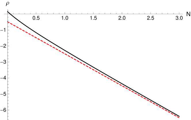
Figure 4: Plot of $\rho(N)$ parameter calculated for the helium atom [black curve, Eq. (18)] compared to its large-$N$ asymptote [red line, Eq. (59)]. The corresponding curves for the other helium-like ions were not included since they are barely distinguishable with the adopted scale of the plot.

This result is independent of the values of $E$, $\alpha$ and $Z$. Figure 4 presents the shape of $\rho(N)$ calculated for the helium atom with an optimized parameter $\alpha$. One can see that the convergence toward the linear asymptote is fast, so that even for $N$ being as small as $3.0$ the error resulting from the use of Eq. (59) is of the order of $1\%$. Therefore, for longer expansions of $\phi(r)$, the approximation (59) is sufficiently accurate for all practical purposes.

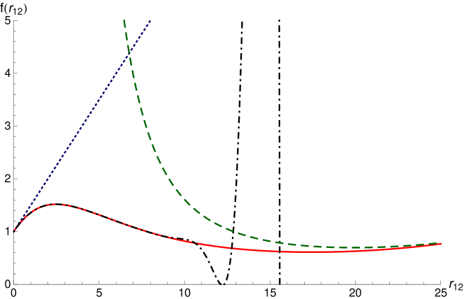
Figure 5: The correlation factor $f(r)$ calculated for the helium atom by using the wave function (44) ($N=2$) and $\alpha=1.920904$. Red solid line is the result of the numerical propagation of the corresponding differential equation. Black dotted line is the variational solution with $f(r)$ expanded in the powers of $r$. Green dashed line is the leading term of the asymptotic expansion of $f(r)$ calculated for the relevant values of the parameters [see Eqs. (46) and (47)]. Blue dotted line ($1+\frac{1}{2}r$) is plotted for the comparison purposes.

To verify our findings numerically, we derived explicit differential equation for $f(r)$ in the case of $N=2$, i.e., a three-term SCF orbital used with in Eq. (45). With the optimized parameter $\alpha=1.920904$ and $N=2$ we obtained the SCF energy equal to $-2.86159$ which compares well with the Hartree-Fock limitszalewicz81 of $-2.86168$. Figure 5 presents results of the numerical propagation of the differential equation for $f(r)$ in the described case. For comparison, we plot the results of the variational calculations with $f(r)$ expanded in a basis set of the powers of $r$. Excellent agreement between those curves is found for small $r$ albeit for a medium range the variational result becomes unstable and progressively less accurate. A new feature of the correlation factor in the present example is that it is no longer monotonic over the whole domain, as found in the previous models. Instead, it possesses a single maximum for a small $r$ value and then a shallow minimum somewhere at the medium large. The leading term of the asymptotic expansion of $f(r)$ is $r^{\rho}e^{Br}$ with $B=0.220361$ and $\rho=-4.38436$, calculated according to Eqs. (46) and (47). Satisfactory agreement between this term and the propagation curve is found for larger values of $r$.

II.5 The Kutzelnigg Ansatz

In this subsection we extend our approach by considering the following Ansatz:

$$\Psi(r_{1},r_{2},r)=\Psi_{0}(r_{1},r_{2})f(r)+\chi(r_{1},r_{2},r),$$ (60)

where $\Psi_{0}(r_{1},r_{2})$ is a reference function (either a product of simple exponential functions or SCF orbitals) and the complementary function $\chi(r_{1},r_{2},r)$ is an ordinary expansion in a set of orbital products. This form of the wave function with $f(r)$ chosen as $1+\frac{1}{2}r$ was used by Kutzelnigg in his work on the R12 theorykutz85 . To simplify derivations we assume that the complementary wave function $\chi(r_{1},r_{2},r)$ is restricted to the following form

$$\chi(r_{1},r_{2},r)=e^{-\alpha(r_{1}+r_{2})}\sum_{kl}^{M}d_{kl}\,r_{1}^{k}r_{2}^{l}.$$ (61)

The basis set used in the expansion (61) is incomplete due to lack of angular functions. Including them (via even powers of $r$) is straightforward and we shall show later that it will not affect the asymptotic behavior of $f(r)$. To avoid technical complications we make the choice $\Psi_{0}(r_{1},r_{2})=e^{-\alpha(r_{1}+r_{2})}$. The main result of this section can be formulated as follows:

Theorem.

If the wave function for the helium like ions has the form

$$\Psi(r_{1},r_{2},r)=e^{-\alpha(r_{1}+r_{2})}f(r)+e^{-\alpha(r_{1}+r_{2})}\sum_{kl}^{M}d_{kl}\,r_{1}^{k}r_{2}^{l},$$ (62)

then the optimal correlation factor $f(r)$ behaves at large $r$ as $r^{\rho}e^{Br}$, where $\rho$ and $B$ are given by Eqs. (18) and (46), i.e., are the same as in the case of the wave function of Eq. (1).

To prove this theorem we have to analyze a differential equation for $f(r)$. Such an equation is obtained by inserting Eq. (60) into the Rayleigh-Ritz functional, evaluating its functional derivative with respect to $f(r)$ and equating this derivative to zero. The resulting equation reads:

$$\begin{split}&\int_{0}^{\infty}\!\!\int_{|r_{1}-r|}^{r_{1}+r}\,r_{1}r_{2}\,e^{-\alpha(r_{1}+r_{2})}\left(\hat{H}-E\right)e^{-\alpha(r_{1}+r_{2})}f(r)dr_{2}dr_{1}=\\ -&\int_{0}^{\infty}\!\!\int_{|r_{1}-r|}^{r_{1}+r}r_{1}r_{2}\,e^{-\alpha(r_{1}+r_{2})}\left(\hat{H}-E\right)\chi(r_{1},r_{2})dr_{2}dr_{1}.\end{split}$$ (63)

We assume here that the linear coefficients $d_{kl}$ on the r.h.s. are fixed and have already been optimized by solving appropriate algebraic equations involving the optimal $f(r)$.

The homogeneous, left-hand side of the above equation is the same as in Eq. (7), except for an additional factor of $-e^{-2\alpha r}/(48\alpha^{3})$. The inhomogeneity on the r.h.s., which we will further denote by $G(r)$, can be easily expressed through the combinations of auxiliary integrals $I_{mn}(2\alpha,2\alpha)\equiv I_{mn}$ evaluated in Appendix A. The result reads:

$$\begin{split}G(r)&=\sum_{kl}^{M}d_{kl}\big{[}\left(\alpha^{2}+E-{1\over r}\right)I_{k+1,l+1}-\alpha(k+1)I_{k,l+1}-\alpha(l+1)I_{k+1,l}\\ &+\frac{1}{2}k(k+1)I_{k-1,l+1}+\frac{1}{2}l(l+1)I_{k+1,l-1}+Z(I_{k,l+1}+I_{k+1,l})\big{]}.\end{split}$$ (64)

According to Eq. (89) from the Appendix A each of the integrals $I_{mn}$ appearing in the equation above is a finite order polynomial in $r$ multiplied by the exponential function $e^{-2\alpha r}$. Therefore, the inhomogeneity $G(r)$ is also a polynomial [of the $(2M+3)$th order] times $e^{-2\alpha r}$. Substituting this form of $G(r)$ into Eq.(63), using Eq. (7) to represent the homogeneous part of Eq.(63) and canceling the exponential factors we find the following differential equation for $f(r)$:

$$\begin{split}&\big{[}-3+3\left(4\alpha Z-2\alpha-3\alpha^{2}+E\right)r+2\alpha\left(12\alpha Z-2\alpha-9\alpha^{2}+3E\right)r^{2}+4\alpha^{2}\left(\alpha^{2}+E\right)r^{3}\big{]}f(r)\\ &+\big{[}6+12\alpha r+4\alpha^{2}r^{2}-8\alpha^{3}r^{3}\big{]}f^{\prime}(r)+r\big{[}3+6\alpha r+4\alpha^{2}r^{2}\big{]}f^{\prime\prime}(r)=-48\alpha^{3}\sum_{k=0}^{2M+3}g_{k}\,r^{k}.\end{split}$$ (65)

where the coefficients $g_{k}$ can be easily expressed through $d_{kl}$ and the $C_{mn}$ coefficients of Appendix A.

It is known that the general solution of an inhomogeneous differential equation is given by a linear combination of the solutions of the homogeneous problem plus any particular solution. To find this particular solution, denoted by $f_{S}(r)$, we try a finite order polynomial as an educated guess

$$f_{S}(r)=\sum_{k=0}^{2M+3}h_{k}\,r^{k}.$$ (66)

Equations determining the coefficients $h_{k}$ are found by inserting the above Ansatz into the differential equation (LABEL:inh4) and gathering the factors multiplying the same powers of $r$. The first three of these equations are

$$\begin{split}&-h_{0}+2h_{1}+16\alpha^{3}g_{0}=0,\\ &3h_{0}\left(-2\alpha-3\alpha^{2}+E+4\alpha Z\right)+h_{1}\left(4\alpha-1\right)+6h_{2}+16\alpha^{3}g_{1}=0,\\ &\alpha h_{0}\left(-4\alpha-18\alpha^{2}+6E+24\alpha Z\right)+h_{1}\left(-6\alpha-5\alpha^{2}+3E+12\alpha Z\right)\\ &+3h_{2}\left(12\alpha-1\right)+36h_{3}+48\alpha^{3}g_{2}=0\end{split}$$ (67)

and the general form is

$$\begin{split}&4\alpha^{2}\left(\alpha^{2}+E\right)h_{n}-2\alpha\left[2\alpha+\left(13+4n\right)\alpha^{2}-3E-12\alpha Z\right]h_{n+1}\\ &+\left[-6\alpha+\alpha^{2}(2n+1)(2n+7)+3E+12\alpha Z\right]h_{n+2}+\left[-3+6\alpha(n+4)(n+3)\right]h_{n+3}\\ &+3(n+4)(n+5)h_{n+4}+48\alpha^{3}g_{n}=0.\end{split}$$ (68)

The number of equations is the same as the number of coefficients and the determinant of the system of equations does not vanish. Having found the special solution $f_{S}(r)$, we can write the general solution of Eq. (LABEL:inh4)

$$f(r)=c_{1}f_{1}(r)+c_{2}f_{2}(r)+f_{S}(r),$$ (69)

where $f_{1}(r)$ and $f_{2}(r)$ are the solutions of the homogeneous problem behaving asymptotically as, $e^{(\alpha-\sqrt{-E})r}r^{\rho}$ and $e^{(\alpha+\sqrt{-E})r}r^{\rho^{\prime}}$, respectively, see the discussion around Eqs. (19)-(LABEL:dnrec) in Sec. II.1.

We can fix the value of $c_{2}$ as equal to zero, otherwise the wave function would not be normalizable. Thus, the long-range behavior of $f(r)$ in the present case reads:

$$f(r)\sim c_{1}e^{(\alpha-\sqrt{-E})r}r^{\rho}+f_{S}(r),$$ (70)

where $c_{1}$ can be fixed by normalization. Since the particular solution is characterized by a polynomial growth and the chosen solution of the homogeneous problem grows exponentially, the leading term of the asymptotic expansion remains exponential. In other words, for a sufficiently large $r$ the behavior of $f(r)$ is always dominated by the exponential growth of the solution to the homogeneous problem. This formally completes the proof of the theorem stated at the beginning of this Section.

It is easy to extend the above theorem by including higher angular momentum functions in the one-electron basis set. One can show that this is equivalent to taking the following form of the complementary wave function

$$\begin{split}\chi(r_{1},r_{2},r)&=e^{-\alpha(r_{1}+r_{2})}\sum_{kl}d_{kl}^{(0)}\,r_{1}^{k}r_{2}^{l}+r^{2}e^{-\alpha(r_{1}+r_{2})}\sum_{kl}d_{kl}^{(1)}\,r_{1}^{k}r_{2}^{l}\\ &+r^{4}e^{-\alpha(r_{1}+r_{2})}\sum_{kl}d_{kl}^{(2)}\,r_{1}^{k}r_{2}^{l}+\ldots\end{split}$$ (71)

This extension does not change the main feature of the differential equation that was used in the proof. Namely, the solution of the homogeneous problem remains unchanged and the inhomogeneity is still a finite-order polynomial in $r$. Therefore, a special solution has the polynomial character and does not contribute to the leading term in the long-range asymptotics.

We also considered another variant of the Kutzelnigg Ansatz:

$$\Psi(r_{1},r_{2},r)=e^{-\alpha(r_{1}+r_{2})}f(r)+e^{-\beta(r_{1}+r_{2})}\sum_{kl}^{M}d_{kl}\,r_{1}^{k}r_{2}^{l},$$ (72)

which differs from the wave function (62) by the choice of different exponent in the complementary part $\chi(r_{1},r_{2},r)$ of the wave function. This additional flexibility is not very effective in the calculations on the helium atom. We checked that the optimal value of $\beta$ is very close to the adopted value of $\alpha$ and the energy gain is insignificant. However, when passing to many-electron systems and using the expansion of pair functions similar to Eq. (72), the splitting of $\alpha$ and $\beta$ corresponds to the use of more diffuse (or more tight) basis set functions in $\Psi(r_{1},r_{2},r)$ than in $\Psi_{0}(r_{1},r_{2})$. This is an important case and therefore the model (72) is worth considering. As before, the extension of (72) by including higher angular momentum functions is simple, so we proceed only with $s$-type functions in the basis.

By repeating the derivation in the previous model, Eqs. (63)-(LABEL:inh4), we find that the differential equation for $f(r)$ is the same as Eq. (LABEL:inh4), except that the inhomogeneity in Eq. (LABEL:inh4) is now given by the function

$$\begin{split}\widetilde{G}(r)=-48\alpha^{3}\,e^{-2(\beta-\alpha)r}\sum_{t=0}^{2M+3}\widetilde{g}_{k}\,r^{k},\end{split}$$ (73)

where $\widetilde{g}_{k}$ are defined in the same way as the $g_{k}$ coefficients in Eq. (LABEL:inh4). The solution of the homogeneous problem is the same as in Subsection II.1. We also found that with appropriate choice of $\widetilde{h}_{k}$ the function

$$\widetilde{f}_{S}(r)=e^{-2(\beta-\alpha)r}\sum_{k=0}^{2M+3}\widetilde{h}_{k}\,r^{k},$$ (74)

is a particular solution of the full equation containing the inhomogeneity $\widetilde{G}(r)$. We can thus use the same arguments as previously and infer that

$$f(r)\sim c_{1}e^{(\alpha-\sqrt{-E})r}r^{\rho}+e^{-2(\beta-\alpha)r}\sum_{k=0}^{2M+3}\widetilde{h}_{k}\,r^{k},$$ (75)

asymptotically for large $r$. The dominant term of this formula depends on the relation between $\alpha$ and $\beta$. In particular the large-$r$ the asymptotics of $f(r)$ is given by

$$f(r)\sim r^{\rho}\,e^{(\alpha-\sqrt{-E})r} \mbox{for}\;\;\;\beta>\beta_{c},$$ (76)

$$f(r)\sim r^{2M+3}\,e^{2(\alpha-\beta)r} \mbox{for}\;\;\;\beta<\beta_{c},$$ (77)

where $\beta_{c}$ is the critical value of $\beta$ equal to

$$\beta_{c}=\frac{1}{2}(\alpha+\sqrt{-E}).$$ (78)

Thus, independently of the choice of $\beta$ we find an exponential growth of $f(r)$ at large $r$.

III Discussion and conclusions

III.1 The “range-separated” model of the correlation factor

The analytic results presented in the previous section can be put into practical use only if a simple analytical form of the correlation factor can be found that mimics, to a good approximation, the exact behavior of $f(r)$ both at small and at large interelectronic distances $r$. This goal is far from being straightforward. This is mainly due to considerable change in the shape of the correlation factor when the function $\Psi_{0}$ is modified. For the simplest possible $\Psi_{0}$ taken as the product of $1s$ orbitals the correlation factor is a monotonically growing function, while for $\Psi_{0}$ taken as an SCF determinant, $f(r)$ exhibits a maximum and minimum before the onset of the monotonic exponential growth. Knowing the behavior of the correlation factor at small and large $r$ we can propose a “range-separated” form with a Gaussian switching

$$f(r)=\big{(}1+\frac{1}{2}r\big{)}\,e^{-\mu r^{2}}+c\,r^{\rho}\,e^{Br}\,S_{n}(\mu r^{2}),$$ (79)

where

$$S_{n}(x)=1-e^{-x}\sum_{l=0}^{n}\frac{x^{l}}{l!}$$ (80)

serves as the “switching function” that interpolates smoothly between the two regimes and the switching is controlled by adjustable parameters $c$ and $\mu$. To eliminate the singularity appearing when $\rho<0$ we take as $n$ the smallest integer satisfying $2n+\rho\geq 0$. For positive $\rho$ we set $n=0$. This form of $f(r)$ is slightly reminiscent of the error-function based range-separation of the Coulomb interaction in the density functional theoryleininger97 . We can increase somewhat the flexibility of this representation by using the Ten-no’s factor at short range:

$$f(r)=\frac{1+2\gamma-e^{-\gamma r}}{2\gamma}\,e^{-\mu r^{2}}+c\,r^{\rho}\,e^{Br}\,S_{n}(\mu r^{2}).$$ (81)

We found that, the analytical form (81) is very flexible. By means of the optimization of the adjustable parameters we are able to obtain a very good analytic fit for each correlation factor discussed in the paper.

When the correlation factor of the form (81) is used in the calculations, new classes of the two-electron integrals arise that were not considered in the literature so far. In these integrals the factors $r^{\rho}$, $e^{-ar}$ and $e^{-ar^{2}}$ are present collectively. For the atomic calculations we managed to express these integrals in terms of the incomplete Gamma and error functions, both in the Slater and Gaussian one-electron basis, and implement them efficiently. These integrals become substantially more difficult when one passes to the many-center molecular systems. The work on evaluating them is in progress in our laboratory.

III.2 Results of exemplary calculations

To check the effectiveness of the “range-separated” representation of Eq. (79) and Eq. (81) we performed variational calculations with the wave function of the form of Eq. (1) and (62). The values of the parameters $B$ and $\rho$ were fixed according to Eqs. (46) and (18). The exponent $\alpha$ was set equal to 1.84833. The parameters $\gamma$, $\mu$ and $c$ were obtained by a least square fit to the exact correlation factor in Eq. (1), obtained from the numerical solution of Eq. (8). We found that for the helium atom $\gamma=0.209587$, $\mu=0.448695$ and $c=1.170940$ are optimal when Eq. (81) is used, whilst for Eq. (79) the values $\mu=0.861347$ and $c=1.169033$ are appropriate.

The results are summarized in Table 2. An inspection of this table shows that accounting for the correct large-$r$ behavior of $f(r)$ via simple formulas of Eq. (79) and Eq. (81) improves significantly the energies obtained with the standard R12 or F12 correlation factors. As expected, the improvement is smaller when the exponential factor with optimized $\gamma$ is used. Note, however, that the optimal value of $\gamma$, equal to 0.2, is in this case much smaller than the value recommended in standard F12 calculationsnoga08 .

It can be seen that with the correlation factor of the form (81) used in the wave function of Eq. (1) we recover about 70% of the correlation energy, so that the expansion in a set of excited state determinants is required only for the remaining 30%. Standard R12 approximation is worse in this respect, recovering about 60%  of the correlation energy.

When the wave function of the form of Eq. (62) is used in the calculations, the obtained energy differences are much smaller but one can see that including the correct asymptotics of $f(r)$ always improves the results. It should be pointed out that in this case the parameters of the correlation factors of Eqs. (79) and (81) were optimized for the wave function of Eq. (1). Nevertheless, the difference between the energy obtained with the approximate correlation factor of Eq. (81) and the fully optimal one, equal to 0.18 milihartree, is smaller than the corresponding difference remaining when using the wave function of Eq. (1). It may also be noted that the energy obtained with the optimal wave function of Eq. (62), i.e, with orbitals of $s$-type symmetry only, is slightly better than the energy from the full CI calculations in the saturated $spdf$ basis setbunge70 ; carrol79 ; weiss61 . With the linear correlation factor the $spd$ limit would be reached with this wave function.

We also performed calculations with Ten-no’s, exponential correlation factor and several values of $\gamma$ which are usually recommended in the literature with $\gamma=1.0$ being the most common choice.noga08 ; skomo11 . Other values, $\gamma=0.5$ and $\gamma=1.5$ were also employedyousaf08 ; rauhut09 ; shiozaki09 . The results are shown in Table 2. On can see that all these choices of $\gamma$ give results worse than the “range-separated” correlation factor of Eq. (81). However, when the exponential correlation factor with optimal $\gamma$ is used in the wave function of Eq. (62) the energy is slightly better than the one obtained with the asymptotically corrected linear correlation factor of Eq.  (79). This is the manifestation of the superiority of the Ten-no’s factor over the linear one at intermediate interelectronic distances.

III.3 Summary and conclusions

In this work we have considered the problem of an optimal form of the correlation factor $f(r)$ for explicitly correlated wave functions, specifically, its asymptotic behavior at large interelectronic distances $r$. We employed the helium atom and helium-like ions as model systems and studied several approximate forms of the the wave function. For the simplest case of the wave function of the form $e^{-\alpha(r_{1}+r_{2})}f(r)$ the optimal correlation factor is exponentially growing function with no extremal points at short range. On the other hand, for the case of an SCF determinant multiplied by the correlation factor, $f(r)$ possesses a single maximum in a small $r$ regime and a minimum at medium $r$ distances. However, in both cases the asymptotic form of the correlation factor is $r^{\rho}e^{Br}$, with $B>0$, so that at large interelectronic distances $f(r)$ diverges exponentially. While the presence of a maximum in the correlation factor for the SCF case has been observed in the study of Tew and Kloppertew05 , neither the presence of the minimum nor the large-$r$ divergence of $f(r)$ have been noticed.

We presented a method to derive a well-defined differential equation for $f(r)$ that can be solved analytically in the large-$r$ regime or alternatively integrated numerically with arbitrary precision using well-developed propagation techniques. The exact analytic information about its solution gives us an opportunity to design new functional form for the correlation factor. We proposed a “range-separated” model where the short- and long-range regimes are approximated by different formulas and sewed together by using a switching function. Simple exemplary calculations with the new form of the correlation factor show that it performs significantly better than the correlation factors used in R12 or F12 methods.

The method proposed in this paper can be a subject to several extensions. First of all, it can be applied to a two-center system to reveal the possible dependence of the correlation factor on the internuclear distance. The second extension goes towards the three-electron atomic systems, such as the lithium atom. This extension may shed some light on the problem of “explicit correlation of triples” considered recently in the literaturekohn09 ; kohn10

To apply the proposed form of the correlation factor in calculations for molecular systems, difficulties concerning the evaluation of the new integrals and application of the RI approximations must be addressed. The work in this direction is in progress in our laboratory. We hope that the proposed models of $f(r)$ will find applications in explicitly correlated atomic and molecular calculations and will help to increase the accuracy of these calculations.

Appendix A Evaluation of auxiliary integrals

In this Appendix we give expressions for the integrals:

$$I_{mn}(\alpha,\beta,r)=\int_{0}^{\infty}\!\!\int_{|r_{1}-r|}^{r_{1}+r}e^{-\alpha r_{1}-\beta r_{2}}r_{1}^{m}r_{2}^{n}dr_{2}dr_{1},$$ (82)

which appear in the derivation of differential equations for $f(r)$. We will assume that $m$ and $n$ are non-negative integers and that $\alpha+\beta>0$. The closed form expressions for the integrals (82) can be obtained most easily by the change of variables $\xi=(r_{1}+r_{2})/r$, $\eta=(r_{1}-r_{2})/r$ and the appropriate change of integration range to $\xi\in[1,+\infty]$ and $\eta\in[-1,+1]$. The absolute value of the Jacobian is $|J|=r^{2}/2$. The integral (82) can now be written as:

$$I_{mn}(\alpha,\beta,r)=\sum_{l=0}^{m}\sum_{k=0}^{n}{m\choose l}{n\choose k}(-1)^{n-k}J_{k+l,m+n-l-k}(\alpha,\beta,r),$$ (83)

where

$$J_{kl}(\alpha,\beta,r)=2\left(\frac{r}{2}\right)^{k+l+2}\,A_{k}(p)\,B_{l}(q),$$ (84)

$A_{k}(p)$ and $B_{k}(q)$ being the well-known integrals:

$$A_{k}(p)= \int_{1}^{\infty}\xi^{k}e^{-p\xi}d\xi=\frac{k!}{p^{k+1}}e^{-p}\sum_{j=0}^{k}\frac{p^{j}}{j!},$$ (85)

$$B_{l}(q)= \int_{-1}^{1}\eta^{l}e^{-q\eta}d\eta=\frac{l!}{q^{l+1}}\left[e^{q}\sum_{j=0}^{l}\frac{(-1)^{j}q^{j}}{j!}-e^{-q}\sum_{j=0}^{l}\frac{q^{j}}{j!}\right]$$ (86)

computed at $p$=$r(\alpha+\beta)/2$ and $q$=$r(\alpha-\beta)/2$. When $\alpha$ =$\beta$, i.e., $q$=$0$ then

$$B_{l}(0)=\frac{1}{l+1}\left[1+(-1)^{l}\right].$$ (87)

In Sec. II.4 we need information about the large $r$ behavior of the integrals $I_{mn}(\alpha,\alpha,r)$. Using Eq. (84) we find

$$J_{kl}(\alpha,\alpha,r)=\frac{e^{-\alpha r}}{\alpha}\left(\frac{r}{2}\right)^{k+l+1}\frac{1+(-1)^{l}}{1+l}\left[1+\frac{k}{\alpha r}+\mathcal{O}\left(\frac{1}{r^{2}}\right)\right].$$ (88)

Inserting this result into Eq. (83) and rearranging summation order we arrive at

$$I_{mn}(\alpha,\alpha,r)=\frac{e^{-\alpha r}}{\alpha}r^{m+n+1}\left[C_{mn}+\frac{D_{mn}}{2\alpha r}+{\mathcal{O}}\left(\frac{1}{r^{2}}\right)\right],$$ (89)

where

$$C_{mn}=\frac{1}{2^{m+n+1}}\sum_{l=0}^{m}\sum_{k=0}^{n}{m\choose l}{n\choose k}\frac{(-1)^{k}+(-1)^{l}}{k+l+1},$$ (90)

and

$$D_{mn}=\frac{1}{2^{m+n}}\sum_{l=0}^{m}\sum_{k=0}^{n}{m\choose l}{n\choose k}\frac{(-1)^{k}+(-1)^{l}}{k+l+1}(m-l+n-k).$$ (91)

Using the formulagarrappa07

$$\sum_{k=0}^{n}{n\choose k}\frac{(-1)^{k}}{k+l+1}=\frac{n!\,l!}{(n+l+1)!}$$ (92)

the summations in Eq. (90) can be carried out and one obtains a simple expression for $C_{mn}$,

$$C_{mn}=\frac{n!\,m!}{(n+m+1)!}.$$ (93)

The corresponding expression for $D_{mn}$ can be obtained from that for $C_{mn}$. After a few simple manipulations one finds that

$$D_{mn}=2(m+n+1)C_{mn}-\delta_{m0}-\delta_{n0},$$ (94)

where $\delta_{ij}$ is the Kronecker symbol.

Appendix B Proof of Eq. (55)

To derive Eq. (55) we have to extract terms proportional to $r^{4N+2}$ that appear in the integrals $M_{1}$ and $M_{2}$. To do so, we need an explicit expression for the remainder $\mathcal{R}_{4N+2}$ in Eq. (55). Representing $M_{1}$ in terms of the $I_{mn}$ integrals and invoking the asymptotic relation (89) one obtains

$$\begin{split}\mathcal{R}_{4N+2}=&f(r)[2\alpha(N+1)I_{2N,2N+1}-2ZI_{2N,2N+1}+r^{-1}I_{2N+1,2N+1}]\\ +&r^{-1}f^{\prime}(r)[(N+2)I_{2N+1,2N+1}+Nr^{2}I_{2N-1,2N+1}-NI_{2N-1,2N+3}]+\mathcal{R}_{4N+1}.\end{split}$$ (95)

We expand now the $I_{mn}$ integrals in Eqs. Eq. (55) and (95) with the help of Eq. (89) and after some rearrangements and simplifications we arrive the following formula for $M_{1}$:

$$M_{1}=r^{4N+2}\,\frac{e^{-2\alpha r}}{2\alpha}\big{[}r\,\Xi_{4N+3}+\Omega_{4N+2}+\mathcal{O}(r^{-1})\big{]},$$ (96)

where

$$\Xi_{4N+3}=-[f(r)(\alpha^{2}+E)-2\alpha f^{\prime}(r)+f^{\prime\prime}(r)]C_{2N+1,2N+1},$$ (97)

cf. Eq. (52) and (53), and

$$\begin{split}\Omega_{4N+2}&=f(r)\Big{[}-\frac{1}{2}(\alpha+\frac{E}{2\alpha})D_{2N+1,2N+1}+2(\alpha N+\alpha-Z)C_{2N,2N+1}+C_{2N+1,2N+1}\Big{]}\\ &-f^{\prime}(r)\Big{[}(N+2)C_{2N+1,2N+1}-\frac{1}{4}D_{2N+2,2N+1}+NC_{2N-1,2N+1}\\ &-NC_{2N-1,2N+3}-\frac{1}{4}D_{2N,2N+1}+\frac{1}{4}D_{2N,2N+3}\Big{]}-\frac{1}{4\alpha}D_{2N+1,2N+1}f^{\prime\prime}(r),\end{split}$$ (98)

The expression for $\Omega_{4N+2}$ can be simplified using Eq. (94) and the following two identities holding for every $N\geq 0$:

$$2(N+1)C_{2N,2N+1}-\frac{1}{2}(4N+3)C_{2N+1,2N+1}=\frac{1}{2}(2N+3)C_{2N,2N+1},$$ (99)

$$NC_{2N-1,2N+1}-NC_{2N-1,2N+3}-(2N+1)C_{2N,2N+1}+(2N+2)C_{2N,2N+3}=0.$$ (100)

The result of these simplifications is

$$\begin{split}\Omega_{4N+2}&=f(r)\Big{[}\frac{\alpha}{2}(2N+3)C_{2N,2N+1}-2ZC_{2N,2N+1}+C_{2N+1,2N+1}\\ &-\frac{E}{2\alpha}(4N+3)C_{2N+1,2N+1}\Big{]}-f^{\prime}(r)C_{2N+1,2N+1}-\frac{4N+3}{2\alpha}C_{2N+1,2N+1}f^{\prime\prime}(r).\end{split}$$ (101)

We still need to determine the last required ingredient – the terms proportional to $r^{4N+2}$ that are in contained $M_{2}$. Expressing $M_{2}$ in terms of $I_{mn}$ integrals we find

$$\begin{split}M_{2}&=-f(r)(\alpha^{2}+E)I_{2N+1,2N}+\frac{1}{2}\alpha\,r^{-1}\,f^{\prime}(r)\Big{[}I_{2N+2,2N}+r^{2}I_{2N,2N}+r^{2}I_{2N+1,2N-1}\\ &+I_{2N+1,2N+1}-I_{2N,2N+2}-I_{2N+3,2N-1}\Big{]}-I_{2N+1,2N}f^{\prime\prime}(r)+\mathcal{R}_{4N+1}.\end{split}$$ (102)

Expansion of every $I_{mn}$ integral according to Eq. (89) gives:

$$M_{2}=r^{4N+2}\,\frac{e^{-2\alpha r}}{2\alpha}\,[\,\Lambda_{4N+2}+\mathcal{O}(r^{-1})\,],$$ (103)

where

$$\Lambda_{4N+3} =-C_{2N+1,2N}\left[(\alpha^{2}+E)f(r)-2\alpha f^{\prime}(r)+f^{\prime\prime}(r)\right].$$ (104)

To derive Eq. (104) we used the following relation holding for every $N\geq 0$:

$$C_{2N,2N}+C_{2N+1,2N-1}+C_{2N+1,2N+1}-C_{2N+3,2N-1}=4C_{2N+1,2N}.$$ (105)

We now have all elements needed to construct the two leading terms of the r.h.s of Eq.  (48). Using Eqs. (96) and (103) one finds that the r.h.s. of Eq.  (48) can be written as

$$c_{N}^{3}\,r^{4N+2}\,\frac{e^{-2\alpha r}}{2\alpha}\big{[}c_{N}\left(r\,\Xi_{4N+3}+\Omega_{4N+2}\right)+4c_{N-1}\,\Lambda_{4N+2}+\mathcal{O}(r^{-1})\big{]},$$ (106)

where $\Xi_{4N+3}$, $\Omega_{4N+2}$ and $\Lambda_{4N+2}$ are given by Eqs. (97), (101) and (104), respectively, and $c_{N}$ and $c_{N-1}$ are defined through Eq. (45). The factor of $4$ in front of $c_{N-1}$ is a result of the symmetry discussed below Eq. (49) and (50). By neglecting the terms of the order lower than $r^{4N+2}$ and equating the remaining ones to zero we obtain the required differential equation for the function that determines the large-$r$ asymptotic behavior of $f(r)$

$$r\,\Xi_{4N+3}+\Omega_{4N+2}+4b_{N}\,\Lambda_{4N+2}=0,$$ (107)

where $b_{N}=c_{N-1}/c_{N}$. Inserting into Eq. (107) the explicit expressions for $\Xi_{4N+3}$, $\Omega_{4N+2}$, and $\Lambda_{4N+2}$, given by Eqs. (97), (101), and (104), dividing by $C_{2N+1,2N+1}$ and using the trivial identity:

$$\frac{C_{2N,2N+1}}{C_{2N+1,2N+1}}=\frac{4N+3}{2N+1},$$ (108)

one arrives at Eq. (55).

Table 1: The values of the parameters $B$ and $\rho$ determining the asymptotic behavior of $f(r)$, Eq. (23). Two approaches were used to fix the exponent $\alpha$: optimization of the energy obtained with the correlated wave function of Eq. (1) and the “bare-nucleus” value $\alpha=Z$.

Z	$\alpha$	$E$	$B$	$\rho$
energy optimized $\alpha$
1	0.84267	$-0.509378$	0.128966	0.322138
2	1.84833	$-2.891254$	0.147959	0.147577
3	2.85039	$-7.268487$	0.154375	0.095543
4	3.85144	$-13.64459$	0.157585	0.070615
5	4.85208	$-22.02025$	0.159510	0.055997
6	5.85251	$-32.39568$	0.160792	0.046391
7	6.85282	$-44.77099$	0.161707	0.039598
8	7.85305	$-59.14622$	0.162393	0.034540
$\alpha=Z$
1	1.00000	$-0.498452$	0.293989	0.124612
2	2.00000	$-2.879363$	0.303131	0.062623
3	3.00000	$-7.256353$	0.306238	0.041754
4	4.00000	$-13.63235$	0.307799	0.031309
5	5.00000	$-22.00795$	0.308737	0.025041
6	6.00000	$-32.38335$	0.309363	0.020864
7	7.00000	$-44.75863$	0.309811	0.017880
8	8.00000	$-59.13384$	0.310147	0.015643

Table 2: Ground-state energies of the helium atom obtained with approximate wave functions of Eqs. (1) and (62). Results obtained with the linear, $1+r/2$, and exponential, $(1+2\gamma-e^{-\gamma r})/(2\gamma)$, correlation factors are denoted by R12 and F12, respectively. The parameter $\gamma$​ =​ 0.2 is close to optimal. Eqs. (79) and (81) are evaluated with $n=0$. The orbital exponent $\alpha$ was always set equal to 1.84833.

$f(r)$	wave function of Eq. (1)	wave of function Eq. (62)
R12	$-2.887447$	$-2.903014$
F12 ($\gamma$=$0.5$)	$-2.886746$	$-2.902976$
F12 ($\gamma$=$1.0$)	$-2.874472$	$-2.900928$
F12 ($\gamma$=$0.2$)	$-2.890349$	$-2.903277$
Eq. (79)	$-2.890886$	$-2.903266$
Eq. (81)	$-2.891048$	$-2.903325$
limit	$-2.891254^{a}$	$-2.903512^{b}$

^aobtained by numerical integration of differential equation
^bobtained by expanding $f(r)$ in powers of $r$ (saturated results, all digits shown are correct).

Figure 1: The correlation factor $f(r)$ calculated for the helium atom using the wave function of Eq. (1) and $\alpha$=1.84833. Red solid line is the result of numerical propagation of Eq. (8). Black dash-dotted line is the variational solution with $f(r)$ expanded in the powers of $r$. Green dashed line is the first term of the asymptotic expansion of $f(r)$. Blue dotted line is used for the short-range factor $1+\frac{1}{2}r$.

Figure 2: The correlation factor $f(r)$ calculated for the helium atom using the wave function of Eq. (25) with $\alpha$=0.321454 and $\beta$=1.968451. The explanation of lines is the same as in Fig. 1, except that the short-range correlation factor, marked by the blue dotted line, in now $1+\frac{1}{4}r$.

Figure 3: The correlation factor $f(r)$ calculated for the helium atom by using the Gaussian wave function of Eq. (32) and $\alpha=0.8598$. Red solid line is the result of numerical solution of the differential equation (33). Black doted-dashed line is the variational solution with $f(r)$ expanded in the powers of $r$. Green dashed line is the leading term of the asymptotic expansion of $f(r)$ calculated for the relevant values of parameters. Blue dotted line ($1+\frac{1}{2}r$) is plotted for the comparison purposes. Two different plot ranges are given separately to improve the readability.

References

- (1) C. Hättig, W. Klopper, A. Köhn, and D. P. Tew, Chem. Rev. 112, 4 (2012).
- (2) L. Kong, F. A. Bischoff, and E. F. Valeev, Chem. Rev. 112, 75 (2012).
- (3) T. Kato, Commun. Pure Appl. Math. 10, 151 (1957).
- (4) R. T. Pack and W. Byers Brown, J. Chem. Phys. 45, 556 (1966).
- (5) S. Furnais, M. Hoffmann-Ostenhof, T. Hoffmann-Ostenhof, T. Ø. Sørensen, Commun. Math. Phys. 255, 183 (2005).
- (6) M. Hoffmann-Ostenhof, T. Hoffmann-Ostenhof, H. Stremnitzer, Phys. Rev. Lett. 68, 3857 (1992).
- (7) K. Szalewicz and B. Jeziorski, Mol. Phys. 108, 3091 (2010).
- (8) S. Ten-no, Theor. Chem. Acc. 131, 1070 (2012).
- (9) R. Bukowski, B. Jeziorski, and K. Szalewicz, in Explicitly correlated functions in chemistry and physics. Theory and applications, edited by J. Rychlewski (Kluwer, Dordrecht, 2003), p. 185.
- (10) J. Rychlewski and J. Komasa, in Explicitly correlated functions in chemistry and physics. Theory and applications, edited by J. Rychlewski (Kluwer, Dordrecht, 2003), p. 91.
- (11) S. Bubin, M. Pavanelo, W. C. Tung, K. L. Sharkley, and L. Adamowicz, Chem. Rev. 113, 36 (2013).
- (12) J. C. Slater, Phys. Rev. 31, 333 (1928).
- (13) E. A. Hylleraas, Z. Phys. 54, 347 (1929).
- (14) E. A. Hylleraas, Z. Phys. 54, 469 (1929).
- (15) R. Jastrow, Phys. Rev. 98, 1479 (1955).
- (16) A. Lüchow and J. B. Anderson, Annu. Rev. Phys. Chem. 51, 501 (2000).
- (17) W. M. C Foulkes, L. Mitas, R. J. Needs, and G. Rajagopal, Rev. Mod. Phys. 73, 33 (2001).
- (18) S. A. Kucharski and R. J. Bartlett, Adv. Quantum Chem. 18, 281 (1986).
- (19) R. J. Bartlett and M. Musiał, Rev. Mod. Phys, 79, 291 (2007).
- (20) F. W. Byron and C. J. Joachain, Phys. Rev. 146, 1 (1966).
- (21) K. C. Pan and H. F. King, J. Chem. Phys. 53, 4397 (1970).
- (22) K. C. Pan and H. F. King, J. Chem. Phys. 56, 4667 (1972).
- (23) G. Chałasiński, B. Jeziorski, J. Andzelm, and K. Szalewicz, Mol. Phys. 33, 971 (1977).
- (24) K. Szalewicz and B. Jeziorski, Mol. Phys. 38, 191 (1979).
- (25) K. Szalewicz, B. Jeziorski, H. J. Monkhorst, and J. G. Zabolitzky, Chem. Phys. Lett. 91, 169 (1982).
- (26) K. Szalewicz, B. Jeziorski, H. J. Monkhorst, and J. G. Zabolitzky, J. Chem. Phys. 79, 5543 (1983).
- (27) B. Jeziorski, K. Szalewicz, H. J. Monkhorst, and J. G. Zabolitzky, J. Chem. Phys. 81, 368 (1984).
- (28) L. Adamowicz and A. J. Sadlej, J. Chem. Phys. 67, 4298 (1977).
- (29) L. Adamowicz and A. J. Sadlej, J. Chem. Phys. 69, 3992 (1978).
- (30) L. Adamowicz, Int. J. Quantum Chem. 13, 265 (1978).
- (31) R. Bukowski, B. Jeziorski, and K. Szalewicz, J. Chem. Phys. 110, 4165 (1999).
- (32) M. Przybytek, B. Jeziorski, and K. Szalewicz, Int. J. Quantum. Chem. 109, 2872 (2009).
- (33) K. Patkowski, W. Cencek, M. Jeziorska, B. Jeziorski, and K. Szalewicz, J. Phys. Chem. A 111, 7611 (2007).
- (34) K. B. Wenzel, J. G. Zabolitzky, K. Szalewicz, B. Jeziorski, and H. Monkhorst, J. Chem. Phys. 85, 3964 (1986).
- (35) R. Bukowski, B. Jeziorski, S. Rybak, and K. Szalewicz, J. Chem. Phys., 102, 888 (1995).
- (36) W. Kutzelnigg, Theor. Chim. Acta 68, 445 (1985).
- (37) W. Klopper and W. Kutzelnigg, Chem. Phys. Lett. 134, 17 (1987).
- (38) W. Kutzelnigg and W. Klopper, J. Chem. Phys. 94, 1985 (1991).
- (39) J. Noga, W. Kutzelnigg, and W. Klopper, Chem. Phys. Lett. 199, 497 (1992).
- (40) J. Noga and W. Kutzelnigg, J. Chem. Phys. 101, 7738 (1994).
- (41) W. Klopper and J. Noga, in Explicitly correlated functions in chemistry and physics. Theory and applications, edited by J. Rychlewski (Kluwer, Dordrecht, 2003), p. 149.
- (42) W. Klopper and C. C. M. Samson, J. Chem. Phys. 116, 6297 (2002).
- (43) F. R. Manby, J. Chem. Phys. 119, 4607 (2003).
- (44) S. Ten-no, J. Chem. Phys. 121, 117 (2004).
- (45) S. Ten-no and F. R. Manby, J. Chem. Phys. 119, 5358 (2003).
- (46) E. F. Valeev, Chem. Phys. Lett. 395, 190 (2004).
- (47) E. F. Valeev and H. F. Schaefer, J. Chem. Phys. 113, 3990 (2000).
- (48) E. F. Valeev and C. L. Janssen, J. Chem. Phys. 121, 1214 (2004).
- (49) R. J. Gdanitz, Chem. Phys. Lett. 210, 253 (1993).
- (50) R. J. Gdanitz, Chem. Phys. Lett. 283, 253 (1998).
- (51) B. J. Persson and P. R. Taylor, J. Chem. Phys. 105, 5915 (1996).
- (52) B. J. Persson and P. R. Taylor, Theor. Chem. Acc. 97, 240 (1997).
- (53) P. Dahle and P. R. Taylor, Theor. Chem. Acc. 105, 401 (2001).
- (54) A. J. May, E. Valeev, R. Polly, and F. R. Manby, Phys. Chem. Chem. Phys. 7, 2710 (2005).
- (55) A. J. May and F. R. Manby, J. Chem. Phys. 121, 4479 (2004).
- (56) S. Ten-no, Chem. Phys. Lett. 398, 56 (2004).
- (57) T. Shiozaki, G. Knizia, and H.-J. Werner, J. Chem. Phys. 134, 034113 (2011).
- (58) T. Shiozaki and H.-J. Werner, J. Chem. Phys. 134, 184104 (2011).
- (59) S. Ten-no, Chem. Phys. Lett. 447, 185 (2007).
- (60) M. Torheyden and E. F. Valeev, J. Chem. Phys. 131, 171103 (2009).
- (61) T. Shiozaki and H.-J. Werner, J. Chem. Phys. 133, 141103 (2010).
- (62) S. Kedzuch, O. Demel, J. Pittner, S. ten-no, and J. Noga, Chem. Phys. Lett. 511, 418 (2011).
- (63) T. J. Martinez and S. Varganov, J. Chem. Phys. 132, 054103 (2010).
- (64) D. P. Tew and W. Klopper, J. Chem. Phys. 123, 074101 (2005).
- (65) M. Abramowitz, I. A. Stegun, Handbook of Mathematical Functions with Formulas, Graphs, and Mathematical Tables, (Dover, New York, 1972).
- (66) G. Pestka, J. Phys. A: Math. Theor. 41, 235202 (2008).
- (67) G. Arfken, “Mathematical Methods for Physicists”, Third Edition, Academic Press, Inc., ISBN 0-12-059810-8.
- (68) C. M. Bender and S. A. Orszag, “Advanced Mathematical Methods for Scientists and Engineers: Asymptotic Methods and Perturbation Theory”, Springer-Verlag, ISBN 0-387-98931-5.
- (69) D. Bohm and D. Pines, Phys. Rev. 92, 609 (1953).
- (70) K. Szalewicz and H.J. Monkhorst, J. Chem. Phys. 75, 5785 (1981).
- (71) T. Leininger, H. Stoll, H.-J. Werner, and A. Savin, Chem. Phys. Lett. 275, 151 (1997).
- (72) D. P. Carrol, H. J. Silverstone, R. M. Metzger, J. Chem. Phys. 71, 4142 (1979).
- (73) C. F. Bunge, Theoret. Chim. Acta (Berl.) 16, 126 (1970).
- (74) A. Weiss, Phys. Rev. 122, 1826 (1961).
- (75) J. Noga, S. Kedžuch, J. Šimunek, and S. Ten-no, J. Chem. Phys. 128, 174103 (2008).
- (76) W. Skomorowski, F. Pawłowski, T. Korona, R. Moszynski, P. S. Żuchowski, and J. M. Hutson, J. Chem. Phys. 134, 114109 (2011).
- (77) G. Rauhut, G. Knizia, and H.-J. Werner, J. Chem. Phys. 130, 054105 (2009).
- (78) T. Shiozaki, M. Kamiya, S. Hirata, and E. F. Valeev, J. Chem. Phys. 130, 054101 (2009).
- (79) K. E. Yousaf and K. A. Peterson, J. Chem. Phys. 129, 184108 (2008).
- (80) A. Köhn, J. Chem. Phys. 130, 131101 (2009).
- (81) A. Köhn, J. Chem. Phys. 133, 174118 (2010).
- (82) R. Garrappa, Int. Math. Forum 2, 725 (2007).