Finding Regression Outliers With FastRCS

Abstract

The Residual Congruent Subset (RCS) is a new method for finding outliers in the regression setting. Like many other outlier detection procedures, RCS searches for a subset which minimizes a criterion. The difference is that the new criterion was designed to be insensitive to the outliers. RCS is supported by FastRCS, a fast regression and affine equivariant algorithm which we also detail. Both an extensive simulation study and two real data applications show that FastRCS performs better than its competitors.

and label=u1,url]http://wis.kuleuven.be/stat/robust

1 Introduction

Outliers are observations that depart from the pattern of the majority of the data. Identifying outliers is a major concern in data analysis for at least two reasons. First, because a few outliers, if left unchecked, will exert a disproportionate pull on the fitted parameters of any statistical model, preventing the analyst from uncovering the main structure in the data. Additionally, one may also want to find outliers to study them as objects of interest in their own right. In any case, detecting outliers when there are more than two variables is difficult because we can not inspect the data visually and must rely on algorithms instead.

Formally, this paper concerns itself with the most basic variant of the outlier detection problem in the regression context. The general setting is that of the ordinary linear model:

$$y_{i}=\alpha+\boldsymbol{x}_{i}^{\prime}\boldsymbol{\beta}+\epsilon_{i}\!$$ (1.1)

where $\boldsymbol{x}_{i}\in\mathbf{R}^{p-1}$ and $y_{i}\in\mathbf{R}$ have continuous distributions, $\epsilon_{i}\sim\mathrm{i.i.d.}\;\mathcal{N}(0,\sigma^{2})$ and $\boldsymbol{\theta}:=(\alpha,\boldsymbol{\beta})$. Then, given a $p$-vector $\tilde{\boldsymbol{\theta}}=(a,\boldsymbol{b})$, we will denote the residual distance of $\boldsymbol{x}_{i}$ to $y_{i}$ as:

$$r_{i}(\tilde{\boldsymbol{\theta}})=|y_{i}-a-\boldsymbol{x}^{\prime}_{i}\boldsymbol{b}|.$$ (1.2)

We have a sample of $n$ observations $(\boldsymbol{x}_{i},y_{i})$ with $n>p$, at least $h=\lceil(n+p+1)/2\rceil$ of which are well fitted by Model $\eqref{mcs:lm}$ and our goal is to identify reliably the remaining ones. A more complete treatment of this topic can be found in textbooks (Maronna et al., 2006).

In this article we introduce RCS, a new procedure for finding regression outliers. We also detail FastRCS, a fast algorithm for computing it. The main output of FastRCS is an outlyingness index measuring how much each observation departs from the linear model fitting the majority of the data. The RCS outlyingness index is affine and regression equivariant (meaning that it is not affected by transformations of the data that do not change the ranking of the squared residuals) and can be computed efficiently for moderate values of $p$ and large values of $n$. For easier outlier detection problems, we find that FastRCS yields similar results as state of the art outlier detection algorithms. When considering more difficult cases however we find that the solution we propose leads to much better outcomes.

In the next section we motivate and define the RCS outlyingness and FastRCS. Then, in Section 3 we compare FastRCS to several competitors on synthetic data. In Section 4 we conduct two real data comparisons.

2 The RCS outlyingness index

2.1 Motivation

Given a sample of $n$ potentially contaminated observations $(\boldsymbol{x}_{i},y_{i})$, the goal of FastRCS is to reveal the outliers. It is well known that this problem is also equivalent to that of finding a fit of Model $\eqref{mcs:lm}$ close to the one we would have found without the outliers. Indeed, to ensures that they stand out in a plot of the fitted residuals, it is necessary to prevent the outliers from pulling the fit in their direction. Other equivariant algorithms that share the same objective are FastLTS (Rousseeuw and Van Driessen, 2006) and FastS (Salibian-Barrera and Yohai, 2006).

However, in tests and real data examples, we often encounter situations where the outliers have completely swayed the fit found by FastLTS and FastS yielding models that do not faithfully describe the multivariate pattern of the bulk of the data. Consider the following example. The three panels in Figure 1 depict the same 100 data points $(\boldsymbol{x}_{i},y_{i})$: 70 drawn from Model $\eqref{mcs:lm}$ and 30 drawn from a concentrated cluster of observations. The orange, solid lines in the first two panels depict, respectively, the line corresponding to the fit found by FastLTS (left) and FastS (center), both computed using the R package robustbase (Rousseeuw et al., 2012) with default parameters (the dashed orange lines depict the 95% prediction intervals). In both cases, the fits depicted in the first two panels do not adequately describe –in the sense of Model $\eqref{mcs:lm}$– the pattern governing the distribution of the majority of the data. This is because the outliers have pulled the fits found by FastLTS and FastS so much in their directions that their distances to it no longer reveals them.

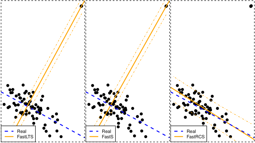
Figure 1: The three panels depict the same data-set. In each panel, the darker blue, dashed line shows the model governing the distribution of the majority –here 70 out of 100– of the observations. The solid orange line shows, respectively, the vector $\theta^{*}$ fitted by each algorithm.

A salient feature of the algorithm we propose is its use of a new measure we call the $I$-index (which we detail in the next section) to select (among many random such subsets) an $h$-subset of uncontaminated data. The $I$-index characterizes the degree of spatial cohesion of a cloud of points and its main advantage lies in its insensitivity to the configuration of the outliers. As we argue below, this makes the FastHCS fit as well as the the outlyingness index derived from it more reliable.

2.2 Construction of the RCS Outlyingness index

The basic outline of the algorithm is as follows. Given an $n$ by $p$ data matrix, FastRCS starts by drawing $M_{p}$ random subsets (’$(p+1)$-subsets’), denoted $\{H^{m}_{0}\}_{m=1}^{M_{p}}$, each of size $(p+1)$ of $\{1,\ldots,n\}$. Then, the algorithm grows each $H^{m}_{0}$ into a corresponding $H^{m}$, a subset of size $h$ of $\{1,\ldots,n\}$ (the letter $H$ without a subscript will always denote a subset of size $h$ of $\{1,\ldots,n\}$). The main innovation of our approach lies in the use of the $I$-index, a new measure we detail below, to characterize each of these $H^{m}$’s. Next, FastHCS selects $H^{*}$, the $H^{m}$ having smallest $I$-index. Then, the $h$ observations with indexes in $H^{*}$ determine the so-called raw FastRCS fit. Finally, we apply a one step re-weighting to this raw FastRCS fit to get the final FastRCS fit. Our algorithm depends on two additional parameters ($K$ and $M_{p}$) but for clarity, these are not discussed in detail until Section 2.3.

We begin by detailing the computation of the $I$-index for a given subset $H^{m}$. Denote $\tilde{\boldsymbol{\theta}}^{mk}$ the coefficients of the hyperplane (the index $k$ identifies these directions) through $p$ data-points from $H^{m}$ (we detail below how we pick these $p$ data-points) and $H^{mk}$ the set of indexes of the $h$ data-points with smallest values of $r_{i}^{2}(\tilde{\boldsymbol{\theta}}^{mk})$:

$$H^{mk}=\{i:r_{i}^{2}(\tilde{\boldsymbol{\theta}}^{mk})\leqslant r_{(h)}^{2}(\tilde{\boldsymbol{\theta}}^{mk})\}$$ (2.1)

where $x_{(h)}$ denotes the $h$-th order statistic of a vector $\boldsymbol{x}$. Then, we define the incongruence index of $H^{m}$ along $\tilde{\boldsymbol{\theta}}^{mk}$ as:

$$I(H^{m},\tilde{\boldsymbol{\theta}}^{mk}):=\log\frac{\displaystyle\operatorname*{ave}_{i\in H^{m}}r_{i}^{2}(\tilde{\boldsymbol{\theta}}^{mk})}{\displaystyle\operatorname*{ave}_{i\in H^{mk}}r_{i}^{2}(\tilde{\boldsymbol{\theta}}^{mk})},$$ (2.2)

with the convention that $\log(0/0):=0$. This index is always positive and will have small value if the vector of $r_{i}^{2}(\tilde{\boldsymbol{\theta}}^{mk})$ of the members of $H^{m}$ greatly overlaps with that of the members of $H^{mk}$. To remove the dependence of Equation (2.2) on $\tilde{\boldsymbol{\theta}}^{mk}$, we measure the incongruence of $H^{m}$ by considering the average over many directions:

$$I(H^{m}):=\operatorname*{ave}_{\tilde{\boldsymbol{\theta}}^{mk}\in B(H^{m})}I(H^{m},\tilde{\boldsymbol{\theta}}^{mk})\;,$$ (2.3)

where $B(H^{m})$ is the set of all regression hyperplanes through $p$ data-points with indexes in $H^{m}$. We call the $H^{m}$ with smallest $I(H^{m})$ the residual congruent subset and denote the index set of its members as $H^{*}$. Next, the raw FastRCS estimates are the parameters $(\boldsymbol{\theta}^{*},\sigma_{*}^{2})$ fitted by OLS to the observations with indexes in $H^{*}$.

In essence, the $I$ index characterizes the homogeneity of the members of a given $h$-subset $H^{m}$ in terms of how much their residuals overlap with those of the $H^{mk}$ over many random regressions. In practice, it would be too laborious to evaluate Equation (2.3) over all members of $B(H^{m})$. A practical solution is to take the average over a random sample of $K$ hyperplanes $\tilde{B}_{K}(H^{m})$ instead. The $I$-index is based on the observation that when the datum with indexes in $H^{m}$ form an homogeneous cloud of points, $\#\{H^{m}\cup H^{mk}\}$ tends to be large over many projection $a^{mk}$, causing $I(H^{m})$ to be smaller.

Consider the example shown in Figure 2. Both panels depict the same set of $n=100$ data-points $(x_{i},y_{i})$. These points form two separate cluster. The main group contains 70 points and is located on the left hand side. Each panel illustrates the behavior of the $I$ index for a given $h$-subset of observations. $H^{1}$ (left) forms a set of homogeneous observations all drawn from the same cluster. $H^{2}$, in contrast, is composed of data points drawn from the two disparate clusters. For each $H^{m}$-subset, $m=\{1,2\}$, we drew two regression lines $\tilde{\boldsymbol{\theta}}^{m1}$ (dark blue, dashed) and $\tilde{\boldsymbol{\theta}}^{m2}$ (light orange). The dark blue dots show the members of $\{H^{m}\cup H^{m1}\}$. Similarly, light orange dots show the members of $\{H^{m}\cup H^{m2}\}$. The diamonds (black squares) show the members of $H^{m1}$ ($H^{m2}$) that do not belong to $H^{m}$. After just two regression, the number of non-overlapping residuals (i.e.{ $\{H^{m}\setminus H^{m1}\}\cap\{H^{m}\setminus H^{m2}\}\}$) is 10 ($m=1$) and 21 ($m=2$) respectively. As we increase the number of regression lines $\tilde{\boldsymbol{\theta}}^{mk}$, this pattern repeats and the difference between an $h$-subset that contains the indexes of an homogeneous cloud of points and one that does not grows steadily.

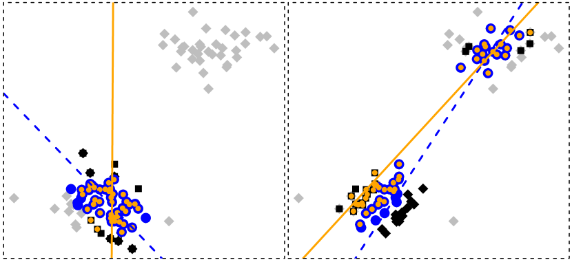
Figure 2: Incongruence index for a subset $H^{1}$ of homogeneous observations (left) and a subset $H^{2}$ of heterogeneous ones (right).

For a given $h$-subset $H^{m}$, the $I$ index measures the typical size of the overlap between the members of $H^{m}$ and those of $H^{mk}$. Given two vector of coefficients $\tilde{\boldsymbol{\theta}}^{m1}$, $\tilde{\boldsymbol{\theta}}^{m2}$, the members of $H^{m1}$ and $H^{m2}$ not in $H^{m}$ (shown as diamonds and black squares in Figure 2) will decrease the denominator in Equation $\eqref{mcs:crit1}$ without affecting the numerator, increasing the overall ratio. Consequently, $h$-subsets whose members form an homogeneous cloud of points will have smaller values of the $I$ index. Crucially, the $I$ index characterizes an $h$-subset composed of observations forming an homogeneous cloud of points independently of the configuration of the outliers. For example, the pattern shown in Figure 2 would still hold if the cluster of outliers were more concentrated. This is also illustrated in the third sub panel in Figure 1 where the parameters fitted by FastRCS are not unduly attracted by members of the cluster of concentrated outliers located on the right.

In Sections 3 and 4, we show that this new characterization allows FastRCS to reliably select uncontaminated $h$-subsets. This includes many situations where competing algorithms fail to do so. First though, the following section details the FastRCS algorithm.

2.3 A Fast Algorithm for the RCS Outlyingness

.

To compute the RCS outlyingness index, we propose the FastRCS algorithm $\eqref{mcs:fmcs}$. An important characteristic of FastRCS is that it can detect exact fit situations: when $h$ or more observations lie exactly on a subspace, FastRCS will return the indexes of an $h$-subset of those observations and the hyperplane fitted by FastRCS will coincide with the subspace.

For each of the $M_{p}$ starting subset $H^{m}_{0}$, Step $b$ grows the size of the corresponding $H^{m}_{l}$ from $p+1$ when $H^{m}_{l}=H^{m}_{0}$ to its final size ($h$) in $L$ steps, rather than in one as is done in FastLTS. We find that this improves the robustness of the algorithm when outliers are close to the good data. We also find that increasing $L$ does not improve performance much if $L$ is greater than 3 and use $L=3$ as default.

 

Algorithm FastRCS (2.4)

 

	for	$m=1$ to $M_{p}$ do:
$a$:		$H^{m}_{0}\leftarrow\{\text{random }$(p+1)$-\text{subset}\}$
$b$:		for	$l=1$ to $L$ do:
			$R_{i}(H^{m}_{l})\leftarrow\displaystyle\operatorname*{ave}_{k=1}^{K}\frac{r_{i}^{2}(\tilde{\boldsymbol{\theta}}^{mk})}{\displaystyle\operatorname*{ave}_{j\in H^{m}_{l}}r_{j}^{2}(\tilde{\boldsymbol{\theta}}^{mk})}\;\;\;1\leq i\leq n$
			set $q\leftarrow\lceil(n-p-1)l/(2L)\rceil+p+1$
			set $H^{m}_{l}\leftarrow\left\{i:R_{i}(H^{m}_{l})\leqslant R_{(q)}(H^{m}_{l})\right\}$
			(‘growing step’)
		end for
		$H^{m}\leftarrow H^{m}_{l}$
$c$:		compute $I(H^{m})\leftarrow\displaystyle\operatorname*{ave}_{k=1}^{K}I(H^{m},\tilde{\boldsymbol{\theta}}^{mk})$
	end for
Keep $H^{*}$, the subset $H^{m}$ with lowest $I(H^{m})$.

 

Empirically also, we found that small values for $K$, the number of elements of $\tilde{B}_{K}(H^{m})$, is sufficient to achieve good results and that we do not gain much by increasing $K$ above 25, so we set $K=25$ as the default. That such a small number of random regressions suffice to reliably identify the outliers is remarkable. This is because the hyperplanes used in FastRCS are fitted to $p$ observations drawn from the members of $H^{m}$ rather than, say, indiscriminately from among the entire set of data-points. Our choice always ensures a wider spread of directions when $H^{m}$ is uncontaminated and this yields better results.

Finally, in order to improve its small sample accuracy, we add a re-weighting step to our algorithm. In essence, this re-weighting strives to award some weight to those observations lying close enough to the model fitted to the members of $H^{*}$. The motivation is that, typically, the re-weighted fit will encompass a greater share of the uncontaminated data. Over the years, many re-weighting procedures have been proposed (Maronna et al., 2006). The simplest is the so called one step re-weighting (Rousseeuw and Leroy, 1987, pg 202). Given an optimal $h$-subset $H^{*}$, we get the final FastRCS parameters by fitting Model $\eqref{mcs:lm}$ to the members of

$$H^{*}_{+}=\{i:r_{i}(\boldsymbol{\theta}^{*})/(\Phi^{-1}(0.75)\operatorname*{med}_{i=1}^{n}r_{i}(\boldsymbol{\theta}^{*}))\leqslant 2.5\}$$ (2.5)

FastLTS and FastS also use a re-weighting step (Rousseeuw and Van Driessen (2006) and Yohai (1987)) and, for all three algorithms, we will refer to the raw estimates as $(\boldsymbol{\theta}^{*},\sigma^{2}_{*})$ and to the final, re-weighted vector of fitted coefficients as $(\hat{\boldsymbol{\theta}},\hat{\sigma}^{2})$.

Like FastLTS and FastS, FastRCS uses many random $(p+1)$-subsets as starting points. The number of initial $(p+1)$-subsets, $M_{p}$, must be large enough to ensure that at least one of them is uncontaminated. For FastLTS and FastS, for each starting $(p+1)$-subset, the computational complexity scales as $O(p^{3}+np^{2})$ –comparable to FastRCS for which it is $O(p^{3}+np)$. The value of $M_{p}$ (and therefore the computational complexity of all three algorithms) grows exponentially with $p$. The actual run times will depend on implementation choices but in our experience are comparable for all three. In practice this means that all three methods become impractical for values of $p$ much larger than 25. This is somewhat mitigated by the fact that they all belong to the class of so called ‘embarrassingly parallel’ algorithms, i.e. their time complexity scales as the inverse of the number of processors meaning that they are particularly well suited to benefit from modern computing environments. To enhance user experience, we implemented FastRCS in C ++   code wrapped in a portable R package (R Core Team, 2012) distributed through CRAN (package FastRCS).

3 Empirical Comparison: Simulation Study

In this section we evaluate the behavior of FastRCS numerically and contrast its performance to that of FastLTS and FastS. For all three, we used their respective R implementation (package robustbase for the last two and FastRCS for FastRCS) with default settings except for the number of starting subsets which for all algorithms we set according to Equation $\eqref{mcs:Ns}$ and the maximum number of iterations for FastS which we increased to 1000. Each algorithm returns a vector of estimated parameters $\hat{\boldsymbol{\theta}}$ as well as a an $h$-subset (denoted $H^{+}$) derived from it:

$$H^{+}=\{i:r_{i}(\hat{\boldsymbol{\theta}})\leqslant r_{(h)}(\hat{\boldsymbol{\theta}})\}$$ (3.1)

Our evaluation criteria are the bias of $\boldsymbol{\theta}^{*}$ and the rate of misclassification of the outliers.

3.1 Bias

Given a central model $\mathcal{F}_{u}$ and an arbitrary distribution $\mathcal{F}_{c}$ (the index $c$ stands for contamination), consider the contamination model:

$$\mathcal{F}_{\varepsilon}=(1-\varepsilon)\mathcal{F}_{u}(y_{u}|\boldsymbol{x}_{u})+\varepsilon\mathcal{F}_{c}(y_{c}|\boldsymbol{x}_{c}),$$ (3.2)

where $\varepsilon$ is the rate of contamination of the sample. The bias measures the differences between the coefficients fitted to $\mathcal{F}_{\varepsilon}$ and those governing $\mathcal{F}_{u}(y_{u}|\boldsymbol{x}_{u})$ and is defined as the norm (Martin et al., 1989):

$$\mbox{bias}(\hat{\boldsymbol{\theta}},\boldsymbol{\theta})=\sqrt{(\hat{\boldsymbol{\theta}}-\boldsymbol{\theta})^{\prime}\mathrm{Var}(\boldsymbol{\theta})^{-1}(\hat{\boldsymbol{\theta}}-\boldsymbol{\theta})},$$ (3.3)

for an affine and regression equivariant algorithm, w.l.o.g., we can set $\mathrm{Var}(\boldsymbol{\theta})=\mathrm{Diag}(p)$ and $\boldsymbol{\theta}=\boldsymbol{0}_{p}$ so that $\eqref{sbias}$ reduces to $||\hat{\boldsymbol{\theta}}||$ and we will use the shorthand $\mbox{bias}(\hat{\boldsymbol{\theta}})$ to refer to it.

Evaluating the bias of an algorithm is an empirical matter. For a given sample, it will depend on the rate of contamination and the distance separating the outliers from the good part of the data. The bias will also depends on the spatial configuration of the outliers (the choice of $\mathcal{F}_{c}$). Fortunately, for affine and regression equivariant algorithms the worst configurations of outliers (those causing the largest biases) are known and so we can focus on these cases.

3.2 Misclassification rate

We can also compare the algorithms in terms of rate of contamination of their final $H^{+}$, the subset of $h$ observations with smallest values of $r_{i}(\hat{\boldsymbol{\theta}})$. Denoting $I_{c}$ the index set of the contaminated observations, the misclassification rate is:

$$\mbox{Mis.Rate}(I_{c},H^{+})=\left.\sum_{i\in H^{+}}\mathcal{I}(i\in I_{c})\middle/\sum_{i=1}^{n}\mathcal{I}(i\in I_{c})\right..$$ (3.4)

This measure is always in $[0,1]$, thus yielding results that are easier to compare across configurations of outliers and rates of contamination. A value of 1 means that $H^{+}$ contains all the outliers. The main difference with the bias criterion is that the misclassification rate does not account for how disruptive the outliers are. For example, when the outliers are close to the good part of the data, it is possible for $\mbox{Mis.Rate}(I_{c},H^{+})$ to be large without a commensurate increase in $\mbox{bias}(\hat{\boldsymbol{\theta}})$.

3.3 Outlier configurations

We generate many contaminated data-sets $(\boldsymbol{X},\boldsymbol{y})$ of size $n$ with $(\boldsymbol{X},\boldsymbol{y})=(\boldsymbol{X}_{u},\boldsymbol{y}_{u})\cup(\boldsymbol{X}_{c},\boldsymbol{y}_{c})$ where $(\boldsymbol{X}_{u},\boldsymbol{y}_{u})$ and $(\boldsymbol{X}_{c},\boldsymbol{y}_{c})$ are, respectively, the genuine and outlying part of the sample. For equivariant algorithms, the worst-case configurations are known. These are the configurations of outliers that are, in a well defined sense, the most harmful. In increasing order of difficulty these are:

• Shift configuration. If we constrain the adversary to (a) set $\sigma^{2}\geq\mathrm{Var}(y_{c}|\boldsymbol{x})$ and (b) place the $y_{c}|\boldsymbol{x}$ at a distance $\nu$ of $\mathrm{E}(y_{u}|\boldsymbol{x})$. Then, the adversary will set $\mathrm{Var}(y_{c}|\boldsymbol{x})=\sigma^{2}$ (Theorem 1 in (Rocke and Woodruff, 1996)) and $\nu$ in order to satisfy (b). Intuitively, this makes the components of the mixture the least distinguishable from one another.

• Point-mass configuration. If we omit constraint (a) above but keep (b), the adversary will place $\boldsymbol{X}_{c}$ on a subspace so that $\mathrm{Var}(y_{c}|\boldsymbol{x})=0$ (Theorem 2 in (Rocke and Woodruff, 1996)). Intuitively, this maximizes the cost of misidentifying any single outlier.

We can generate the $\boldsymbol{X}_{u}$’s and the $\epsilon_{i}$’s from standard normal distributions since all methods under consideration are affine and regression equivariant. Likewise, the $\boldsymbol{X}_{c}$’s are draws from a multivariate normal distribution with $\mathrm{Var}(\boldsymbol{X}_{c})$ equal to $\mathrm{Diag}(p)$ (Shift) or $10^{-4}\mathrm{Diag}(p)$ (Point-mass) and $\mathrm{E}(\boldsymbol{X}_{c})$ set so that $\min_{i\in I_{c}}||\boldsymbol{x}_{i}||=d_{x}\sqrt{\chi^{2}_{0.95;p-1}}$ where $d_{x}$ is either one of 2 (nearby outliers) or 8 (far away outliers). Finally, $\mathrm{Var}(y_{c}|\boldsymbol{x})$ is one of $\sigma^{2}$ or $10^{-4}\sigma^{2}$ depending again on whether the outlier configuration is Shift or Point-mass. Next, for a given value of the parameters in Model $\eqref{mcs:lm}$ and a data matrix $\boldsymbol{X}_{c}$, the bias will depend on the vertical distance between the outliers and the genuine observations. We will place the outliers such that they lie at a distance $\nu$ of the good data:

$$\nu=\min_{i\in I_{c}}\frac{|y_{i}-\mathrm{E}(y_{u}|\boldsymbol{x}_{i})|}{\mathrm{W}(\boldsymbol{x}_{i})}\,\,,$$ (3.5)

where $\mathrm{W}(\boldsymbol{x}_{i})$ is half the asymptotic width of the usual LS prediction interval, evaluated at $\boldsymbol{x}_{i}$. The complete list of simulation parameters follows:

• the dimension $p$ is one of $\{4,8,12,16\}$ and the sample size is $n=25p$,

• the configuration of the outliers is either Shift or Point-mass.

• $\alpha\in\{0.5,0.75\}$ is the proportion of the sample that can be assumed to follow Model $\eqref{mcs:lm}$. In Section 3.4 (Section 3.5) we consider the case where we set $\alpha=0.5$ ($\alpha=0.75$).

• $\varepsilon\in\{0.1,0.2,0.3,0.4\}$ (when $\alpha=0.5$) or $\varepsilon\in\{0.1,0.2\}$ (when $\alpha=0.75$).

• the distance separating the outliers from the good data on the design space is $d_{x}=\{2,8\}$. The distance separating the outliers from $\boldsymbol{x}^{\prime}\boldsymbol{\theta}$ is $\nu=\{1,2,...,10\}$.

• the number of initial $(p+1)$-subsets $M_{p}$ is given by (Maronna et al., 2006)

  $$M_{p}=\log(0.01)/\log(1-(1-\varepsilon_{0})^{p+1})\;,$$ (3.6)

  with $\varepsilon_{0}=4(1-\alpha)/5$ so that the probability of getting at least one uncontaminated starting point is always at least 99 percent.

We also considered other configurations such as so-called vertical outliers ($d_{x}=0$) or where $\nu$ is extremely large (i.e. $\geq 1000$), but they posed little challenge for any of the algorithms, so we do not discuss these results. In Figures 3 to 8 we display the bias (left panel) and the misclassification rate (right panel) for discrete combinations of the dimension $p$, contamination rate $\varepsilon$ and the degree of separation between the outliers and the genuine observations on the design space (which we control through the parameter $d_{x}$). In all cases, we expect the outlier detection problem to become monotonically harder as we increase $p$ and $\varepsilon$. Furthermore, undetected outliers that are located far away from the good data on the design space will have more leverage on the fitted coefficients. For that reason, we also expect the biases to increase monotonically with $d_{x}$. Therefore, not much information will be lost by considering a discrete grid of a few values for these parameters. The configurations also depend on the distance separating the outliers from the true model, which we control through the simulation parameter $\nu$. The effects of $\nu$ on the bias are harder to foresee: clearly nearby outliers will be harder to detect but misclassifying distant outliers will increase the bias more. Therefore, we will test the algorithms for many values (and chart the results as a function) of $\nu$. For both the bias and the misclassification curves, for each algorithm, a solid colored line will depict the median and a dotted line (of the same color) the 75th percentile. Here, each panel will be based on 1000 simulations.

3.4 Simulation results (a)

The first part of the simulation study covers the case where there is no information about the extent to which the data is contaminated. Then, for each algorithm, we have to set the size of the active subset to $h$, corresponding to the lower bound of slightly more than half of the data. For FastLTS and FastRCS there is a single parameter $\alpha$ controling the size of the active subset so that we set $\alpha=0.5$. For FastS, we follow (Rousseeuw and Leroy, 1987, table 19, p. 142) and set the value of the tunning parameters to $(b,c)=(0.5,1.547)$.

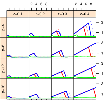
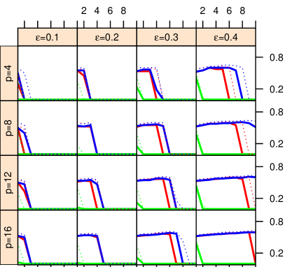
Figure 3: $\mbox{Bias}(\hat{\boldsymbol{\theta}})$ (left) and $\mbox{Mis.Rate}(I_{c},H^{+})$ (right) for Shift contamination, $\varepsilon=\{0.1,\ldots,0.4\}$, $p=\{4,\ldots,16\}$, $d_{x}=2$, $\alpha=0.5$ as a function of $\nu$. FastLTS, FastS, FastRCS.

In Figure 3 we display the $\mbox{Mis.Rate}(I_{c},H^{+})$ and $\mbox{bias}(\hat{\boldsymbol{\theta}})$ curves of each algorithm at $d_{x}=2$ as a function of $\nu$ for different values of $p$ and $\epsilon$ for the Shift configuration. Starting at the second column, the $\mbox{Mis.Rate}(I_{c},H^{+})$ curves are much higher for FastS and FastLTS than for FastRCS but the outliers included in their selected $h$-subsets do not exert enough pull on the fitted model to yield correspondingly large biases. From the the third column onwards, the outliers are now numerous enough to exert a visible pull on the coefficients fitted by FastLTS and FastS. By the fourth column of both panel, the performances of these two algorithms deteriorates further and they now fail to detect even outliers located very far from $\boldsymbol{x}^{\prime}\boldsymbol{\theta}$. Far away outliers, if left unchecked, will exert a larger leverage on the $\hat{\boldsymbol{\theta}}$ and this is visible in the bias curves of FastLTS and FastS which are now much higher. The performance of FastRCS, on the other hand, is not affected by $\nu$, $p$ or $\varepsilon$ and remains comparable throughout.

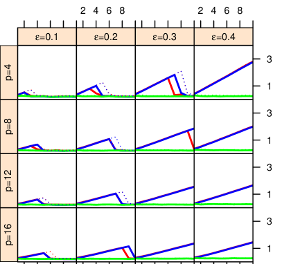
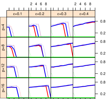
Figure 4: $\mbox{Bias}(\hat{\boldsymbol{\theta}})$ (left) and $\mbox{Mis.Rate}(I_{c},H^{+})$ (right) for Shift contamination, $\varepsilon=\{0.1,\ldots,0.4\}$, $p=\{4,\ldots,16\}$, $d_{x}=8$, $\alpha=0.5$ as a function of $\nu$. FastLTS, FastS, FastRCS.

In Figure 4, we again examine the effects of Shift contamination, but for $d_{x}=8$. Now, starting at $\varepsilon=0.2$ and $p=12$ the $\mbox{Mis.Rate}(I_{c},H^{+})$ curves of FastLTS and FastS show that these algorithms can not seclude even those outliers located within a rather large slab around $\boldsymbol{x}^{\prime}\boldsymbol{\theta}$. Furthermore, from $\varepsilon\geq 0.3$, as the configurations get harder, the maximum of the bias curves clearly show that the parameters fitted by these two algorithms diverge from $\boldsymbol{\theta}$ in an increasingly large range of values of $\nu$. Comparing the $\mbox{Mis.Rate}(I_{c},H^{+})$ curves of FastLTS and FastS in Figure 4 with those in Figure 3, we see that these two algorithms are noticeably less successful at identifying outliers far removed on the design space than nearer ones. In contrast, in Figure 4, we see that the performance of FastRCS is very good both in terms of $\mbox{bias}(\hat{\boldsymbol{\theta}})$ and $\mbox{Mis.Rate}(I_{c},H^{+})$. Furthermore, these measures of performance remain consistently good across the different values of $p$, $\varepsilon$ and $\nu$. Comparing the performance of FastRCS in Figure 4 with the results shown in Figure 3 we also see that our algorithm is unaffected by the greater separation between the outliers and the good data in the $\boldsymbol{X}$ space.

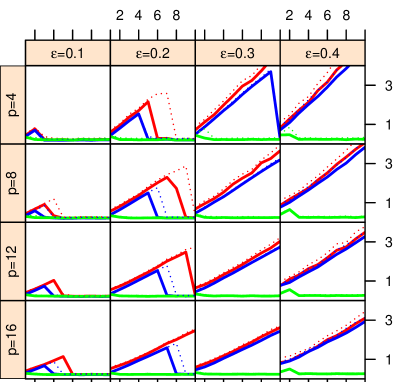
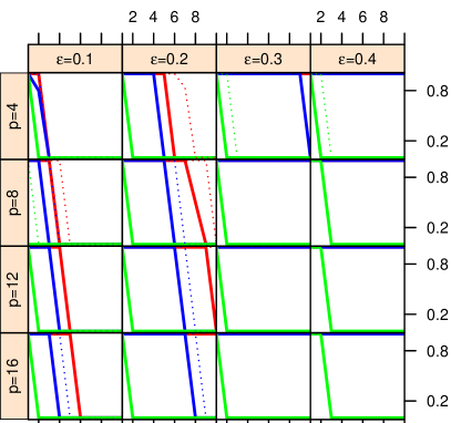
Figure 5: $\mbox{Bias}(\hat{\boldsymbol{\theta}})$ (left) and $\mbox{Mis.Rate}(I_{c},H^{+})$e (right) for Point-mass contamination, $\varepsilon=\{0.1,\ldots,0.4\}$, $p=\{4,\ldots,16\}$, $d_{x}=2$, $\alpha=0.5$ as a function of $\nu$. FastLTS, FastS, FastRCS.

In Figure 5, we show the results for the more difficult case of Point-mass contamination with $d_{x}=2$. As expected, we find that concentrated outliers are causing much higher biases for FastS and FastLTS, especially in higher dimensions. Already when $\varepsilon=0.2$, FastS displays biases that are sensibly higher than their maximum values against the Shift configuration. From $p=8$, both algorithms also yields contaminated $h$-subsets for most values of $\nu$. Looking at the $\mbox{Mis.Rate}(I_{c},H^{+})$ curves of these two algorithm, we also see that in many of cases, the optimal $h$-subsets selected by FastLTS and FastS actually contain a higher fraction of outliers than the original sample. In contrast, for FastRCS, the performance curves in Figure 5 are essentially similar to those shown in Figure 3, attesting again that our algorithm is not unduly affected by the spatial concentration of the outliers.

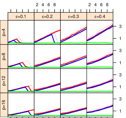
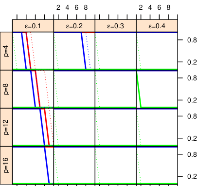
Figure 6: $\mbox{Bias}(\hat{\boldsymbol{\theta}})$ (left) and $\mbox{Mis.Rate}(I_{c},H^{+})$ (right) for Point-mass contamination, $\varepsilon=\{0.1,\ldots,0.4\}$, $p=\{4,\ldots,16\}$, $d_{x}=8$, $\alpha=0.5$ as a function of $\nu$. FastLTS, FastS, FastRCS.

In Figure 6, we examine the effects of Point-mass contamination for $d_{x}=8$. As in the case for Shift contamination, we see that an increase in $d_{x}$ entails a decline in performance for both FastLTS and FastS with high maximum values of the bias curves now starting at $\varepsilon\geq 0.2$ already. In terms of $\mbox{Mis.Rate}(I_{c},H^{+})$ curves, too, both algorithm have their weakest showings, with selected subsets that have a higher rate of contamination that the original data-sets for most values of $\nu$ starting from the middle rows of the first column already. As before, the lower rate of outlier detection combined with the greater separation of the outliers on the design space means that the bias curves of FastLTS and FastS are worse than those shown in Figure 5. Again, contrast this with the behavior of FastRCS which maintains low and constant bias and misclassification curves throughout. Further comparing the performance curves of FastRCS for the configuration considered in Figure 6 to those considered in Figures 5 and 4 we see, again, that FastRCS is not affected by either the spatial concentration or the degree of separation of the outliers.

3.5 Simulation results (b)

In this section, we now consider the case, important in practice, where the user can confidently place an upper bound on the rate of contamination of the sample. To fix ideas, we will set the proportion of the sample assumed to follow Model $\eqref{mcs:lm}$, to approximately $3/4$ so that in this section $\#H^{*}\approx 3h/2$. For FastLTS and FastRCS we adapt the algorithms by setting their respective $\alpha$ parameter to 0.75. For FastS, we again follow (Rousseeuw and Leroy, 1987, table 19, p. 142) and now set $(b,c)=(0.75,2.937)$. For all three algorithms we also reduce the number of starting subsets by setting $\varepsilon_{0}=0.2$ in Equation $\eqref{mcs:Ns}$. Then, as before, we will measure the effects of the various configurations of outliers on the algorithms (but now for $\varepsilon\in\{0.1,0.2\}$).

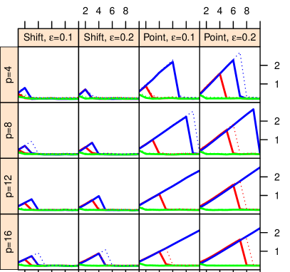
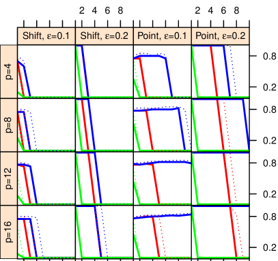
Figure 7: $\mbox{Bias}(\hat{\boldsymbol{\theta}})$ (left) and $\mbox{Mis.Rate}(I_{c},H^{+})$ (right) for Shift and Point-mass contamination, $\varepsilon=\{0.1,0.2\}$, $p=\{4,\ldots,16\}$, $\alpha=0.75$, $d_{x}=2$ as a function of $\nu$. FastLTS, FastS, FastRCS.

Figure 7 summarizes the case where $d_{x}=2$. The first two columns of $\mbox{bias}(\hat{\boldsymbol{\theta}})$ (left) and $\mbox{Mis.Rate}(I_{c},H^{+})$ contain results for the Shift configuration, and the last two, for Point-mass. For the Shift configuration, when the outliers are far from the hyperplane fitting the good part of the data, all methods have low biases. Though FastS and FastLTS still deliver optimal $h$-subsets that are heavily contaminated by outliers, these do not exert a large enough pull on the $\hat{\boldsymbol{\theta}}$ to affect the biases. Generally all methods yield results that are comparable with the corresponding cases shown in Figure 3. In the case of Point-mass contamination (shown in the last two columns), FastLTS and FastS again experience greater difficulty with the Point-mass configuration and results are worse than those shown in Figure 5 for the corresponding settings. Again, the results for FastRCS remains similar to those depicted in Figure 5.

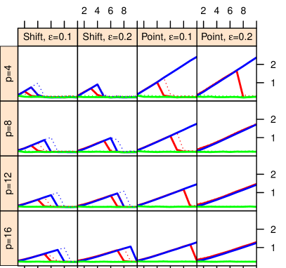
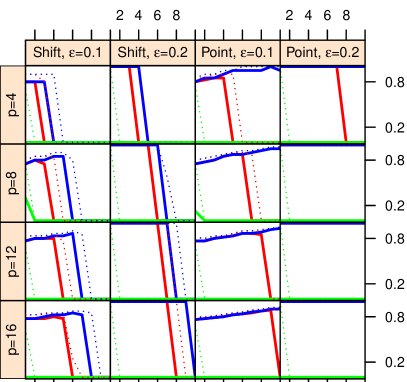
Figure 8: $\mbox{Bias}(\hat{\boldsymbol{\theta}})$ (left) and $\mbox{Mis.Rate}(I_{c},H^{+})$ (right) for Shift and Point-mass contamination, $\varepsilon=\{0.1,0.2\}$, $p=\{4,\ldots,16\}$, $\alpha=0.75$, $d_{x}=8$ as a function of $\nu$. FastLTS, FastS, FastRCS.

Figure 8 depicts the simulation results for $\alpha=0.75$ when $d_{x}=8$. As before, this places additional strain on FastLTS and FastS. In the case of Shift contamination, the results for these two algorithms are qualitatively the same as in Figure 4. For FastLTS and FastS, the results are worst for Point-mass contamination and show, again, a clear deterioration vis-á-vis Figure 6. Now, FastLTS fails to identify the outliers in any but the easiest configuration, and FastS performs poorly in all configurations. In contrast, FastRCS yields the same performance, whether it is measured in terms of $\mbox{bias}(\hat{\boldsymbol{\theta}})$ or $\mbox{Mis.Rate}(I_{c},H^{+})$, as those obtained in the same configurations, but with a higher value of $\alpha$.

Overall in our tests, we observed that FastLTS and FastS both exhibit considerable strain. In many situations these two algorithms yield optimal $h$-subsets that are so heavily contaminated as to render them wholly unreliable for finding the outliers. In these situations, both algorithm also invariably yield vectors of fitted parameters $\hat{\boldsymbol{\theta}}$ that are completely swayed by the outliers and, consequently, very poorly fit the genuine observations. We note that as the configurations become more challenging, the bias curves for FastLTS and FastS deviate upward, and the $\mbox{Mis.Rate}(I_{c},H^{+})$ curves advance to the right in a systemic manner. We observe no corresponding effect for FastRCS. These quantitative differences between FastRCS and the other two algorithms, repeated over adversary configurations, lead us to interpret them as indicative of a qualitative difference in robustness.

4 Empirical Comparison: Case Studies

In the previous section, we compared FastRCS to two state of the art outlier detection algorithms in situations that were designed to be most challenging for equivariant procedures. In this section, we will also compare FastRCS to FastLTS and FastS, but this time using two real data examples. The first illustrate the use of FastRCS in situations where $n/p$ is small (typically these situations are particularly challenging for anomaly detection procedures) while the second example illustrates the use of FastRCS in situations where $p$ is large.

4.1 Slump Data

In this section, we consider a real data problem from the field of engineering: the Concrete ”Slump” Test Data set (Yeh, 2007). This data-set consists of 7 input variables measuring the quantity of cement, fly ash, blast furnace slag, water, super-plasticizer, coarse aggregate, and fine aggregate used to make the corresponding variety of concrete. Finally, we use 28-day compressive strength as response variable. The ”Slump” data-set is actually composed of two class of observations collected over two separate periods with the first set of measurements predating the second ones by several years. After excluding several data-points that are anomalous in that the values of either the slag and fly ash variable is exactly zero, we are left with 59 measurements, with first 35 data (last 24) points belonging to the set $J_{O}$ ($J_{N}$) of older (newer) observations. In this exercise, we will hide the vector of class labels, in effect casting the members of $J_{N}$ as the outliers and the task of all the algorithms will be to reveal them.

To ensure reproducibility we ran all algorithms with option seed=1 and default values of the parameters (except for the number of starting subset $M_{p}$ which we set according to Equation (3.6)) and included both data-sets used in this section in the FastRCS package. For all three algorithms, we will denote as $\hat{\boldsymbol{\theta}}_{j}$ the fit found by algorithm $j$, $\hat{H}_{j}=\{i:r_{i}(\hat{\boldsymbol{\theta}}_{j})/\hat{\sigma}_{j}\leqslant 2.5\}$ will denote the subset of observations classified as ”good” and $\hat{H}_{\setminus j}=\{\{1,\ldots,n\}\setminus\hat{H}_{j}\}$ its complement.

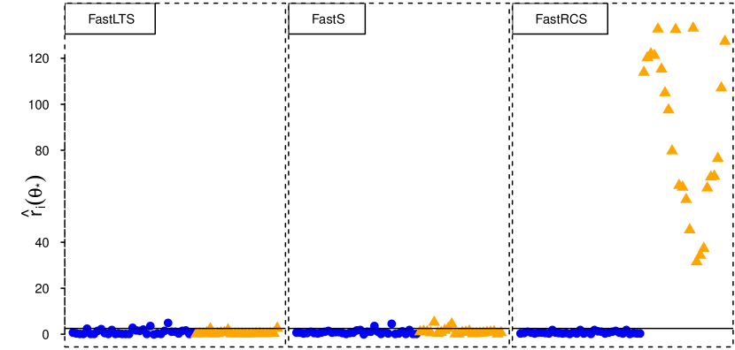
Figure 9: Residual distances $r_{i}(\hat{\boldsymbol{\theta}}_{j})/\hat{\sigma}_{j}$ for the FastLTS (left), FastS (middle), and FastRCS (right), ran on the ”Slump” data-set. In each panel, the dark blue (light orange) dots (triangles) depict the $r_{i}(\hat{\boldsymbol{\theta}}_{j})/\hat{\sigma}_{j}$ values for the members of $J_{O}$ ($J_{N}$).

Next, we ran all three algorithms on the ”Slump” data-set, using $M_{p}=500$. In Figure 9, we display the standardized residual distance $r_{i}(\hat{\boldsymbol{\theta}}_{j})/\hat{\sigma}_{j}$, for each algorithm in a separate panel. The dark blue residual (light orange) points (triangles) depict the $r_{i}(\hat{\boldsymbol{\theta}}_{j})/\hat{\sigma}_{j}$ for the 35 members of $J_{O}$ (24 members of $J_{N}$). An horizontal line at $2.5$ shows the usual outlier rejection threshold. For both FastLTS and FastS, the values of the $r_{i}(\hat{\boldsymbol{\theta}}_{j})/\hat{\sigma}_{j}$ (shown in the left and middle panel of Figure 9 respectively) corresponding to the members of $J_{O}$ and $J_{N}$ largely overlap. As a result, in both cases, the optimal $h$-subset includes both members of $J_{N}$ and $J_{O}$. Looking at the composition of the $H^{+}$ subset found by FastLTS, we see that it contains 19 (out of $h=34$) members of $J_{N}$. For FastS, $H^{+}$ contains 13 members of $J_{N}$. Considering now the observations classified as good (the members of $\hat{H}_{j}$) by both algorithms, we see that FastLTS (FastS) finds only 15 (5) outliers. The outliers found by both approaches are well separated from the fitted model (the nearest outlier lies at a standardized residuals distance of $2.9$ for both algorithms) but they tend to be located near the good observations on the design space. For example, the nearest outlier lie at a Mahalanobis distance of $0.7\sqrt{\chi^{2}_{0.95,7}}$ wrt to the members of $\hat{H}_{\text{FastLTS}}$ and $0.6\sqrt{\chi^{2}_{0.95,7}}$ wrt to the members of $\hat{H}_{\text{FastS}}$. Finally, the members of the $\hat{H}_{j}$ subsets identified by both algorithms contains, again, many members of $J_{N}$: 21 (out of $|\hat{H}_{\text{FastLTS}}|=44$) for $\hat{H}_{\text{FastLTS}}$ and 21 (out of 54) for $\hat{H}_{\text{FastS}}$.

In contrast to the innocent looking residuals seen in the first two panels of Figure 9, the plot of the $r_{i}(\hat{\boldsymbol{\theta}}_{j})/\hat{\sigma}_{j}$ corresponding to the FastRCS fit (shown in rightmost panel), clearly reveals the presence of many observations that do not follow the multivariate pattern of the bulk of the data. For example, the outliers identified by FastRCS are much more distinctly deviating from the pattern set by the majority of the data than those identified by FastS and FastLTS: the nearest outlier now stands at $r_{i}(\hat{\boldsymbol{\theta}}_{j})/\hat{\sigma}_{j}=32$. Furthermore, the composition of these two groups is now consistent with the history of the ”Slump” data-set as the $H^{+}$ found by FastRCS is solely populated by members of $J_{O}$ and $\hat{H}_{\text{FastRCS}}$ contains all the (and only those) 35 observations from $J_{O}$. Interestingly, the two groups of observations identified by FastRCS are clearly distinct on the design space where they form two well separated cluster of roughly equal volume on the design space. For example, the closest member of $\hat{H}_{\setminus\text{FastRCS}}$ lies at a Mahalanobis distance of over $19\sqrt{\chi^{2}_{0.95,7}}$ wrt the members of $\hat{H}_{\text{FastRCS}}$.

The blending of members of both $J_{N}$ and $J_{O}$ in both $\hat{H}_{\text{FastLTS}}$ and $\hat{H}_{\text{FastS}}$ despite the large separation between the members $J_{N}$ and those from $J_{O}$, on the design space as well as to the hyperplane fitting the observations with indexes in $J_{O}$ together suggest that the optimal subset selected by both FastLTS and FastS do in fact harbor many positively harmful outliers.

Consecutively, because the outliers in this example are well separated from the bulk of the data, the presence of even a handful of them in $\hat{H}_{\text{FastLTS}}$ ($\hat{H}_{\text{FastS}}$) indicates that they have pulled the resulting fits so much in their direction as to render parameters fitted by both algorithms altogether unreliable.

4.2 The ”Don’t Get Kicked!” data-set

In this subsection, we illustrate the behavior of FastRCS on a second real data problem from a commercial application: the ”Don’t Get Kicked!” data-set (Kaggle, 2012). This data-set contains thirty-four variables pertaining to the resale value of 72,983 cars at auctions. Of these, we use of the continuous ones to model the sale price of a car as a linear function of eight measures of current market acquisition prices, the number of miles on the odometer and the cost of the warranty. More specifically, we consider as an illustrative example all 488 data-points corresponding to sales of the Chrysler Town & Country but the pattern we find below repeats for many other cars in this data-set. We ran all three algorithms on the data-set (with $M_{p}=3000$) and, in Figure 10, we plot the vector of fitted standardized residual distance $r_{i}(\hat{\boldsymbol{\theta}}_{j})/\hat{\sigma}_{j}$ returned by each in a separate panel together with, again, an horizontal line at $y=2.5$ demarcating the usual outlier rejection threshold. Finally, for each algorithm, we also show the observations flagged as influential as light orange triangles.

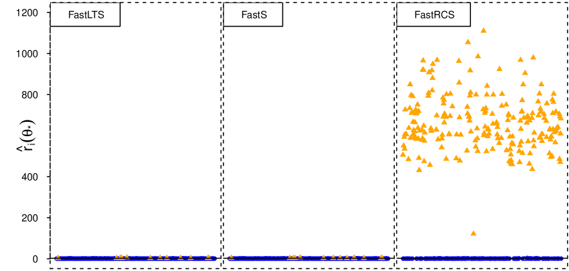
Figure 10: Residual distances $r_{i}(\hat{\boldsymbol{\theta}}_{j})/\hat{\sigma}_{j}$ for the FastLTS (left), FastS (middle), and FastRCS (right), obtained on the ”Don”t get kicked!” data-set. In each panel, the light orange triangles depict those observations for which $r_{i}(\hat{\boldsymbol{\theta}}_{j})/\hat{\sigma}_{j}>2.5$.

We first discuss the results of FastLTS and FastS jointly (shown in the left and middle panel of Figure 10 respectively) since they are broadly similar. Here again, the first two panels depict a reasonably well behaved data-set with very few harmful outliers. Overall the number of data points for which $r_{i}(\hat{\boldsymbol{\theta}}_{j})/\hat{\sigma}_{j}$ is larger than 2.5 is 13 for FastLTS and 14 for FastS. These are quiet close to the the fitted $\hat{\boldsymbol{\theta}}$ and the smallest value of $r_{i}(\hat{\boldsymbol{\theta}}_{j})/\hat{\sigma}_{j}$ for the outliers is $2.5$ for both algorithms (the second nearest lies at a standardized distance of $2.6$). Furthermore, these outliers are close, on the design space, to the majority of the data. For example, for both algorithms, the nearest outlier lies at a Mahalanobis distance of $0.4\sqrt{\chi^{2}_{0.95,10}}$ wrt to the good observations (the second closest is located at a distance of $0.5\sqrt{\chi^{2}_{0.95,10}}$). Overall, both algorithms suggest that observations forming the Don’t Get Kicked! data-set is broadly consistent with Model $\eqref{mcs:lm}$ except for $\approx 2$% of outliers.

In this example again, we find that the FastRCS fit reveals a much more elaborate structure to this data-set. In this case, $\hat{H}_{\text{FastRCS}}$ is composed of 262 observations, barely more than $h=250$ which imply a data-set beset by outliers. Furthermore, even a cursory inspection of the standardized residuals clearly reveals the presence of a large group of observations not following the multivariate pattern of the bulk of the data. Surprisingly in the light of the fit found by the other algorithms, we find that the outliers identified by FastRCS in this data-set are actually very far from the model fitting the bulk of the data. Setting aside row 171 (visible on the right panel of Figure 10 as the isolated outlier lying somewhat closer to the genuine observations), we find that the nearest outlier lies at a standardized residual distance of over 120 wrt to the FastRCS fit on the model space. Considering now the design space alone, we find that here too the members of $\hat{H}_{\text{FastRCS}}$ are clearly separated from the bulk of the data: we find that the nearest outlier (again setting observation 171 aside) lies at a Mahalanobis distance of over $685\sqrt{\chi^{2}_{0.95,10}}$ wrt to the members of $\hat{H}_{\text{FastRCS}}$.

A salient feature of this exercise is that the outliers in the ”Don’t get kicked!” data-set are genuine discoveries in the sense that when examining the variables (including the qualitative ones not used in this analysis), we could not find any single one exposing them, yet they materially affect the model. As with the ”Slump” data-set, the ”Don’t Get Kicked!” data-set is also interesting because the outliers identified (exclusively) by FastRCS are not analogous to the worst case configurations we considered in the simulations. Indeed, far from resembling the concentrated outliers we know to be most challenging for FastS and FastLTS, the members of $\hat{H}_{\setminus\text{ FastRCS}}$ seem to form a scattered cloud of points, occupying a much larger volume on the design space than the members of the main group. Nevertheless, here too, the fit found by both FastLTS and FastS lumps together observations stemming from very disparate groups. In this case too, the large separation between the members of $\hat{H}_{\text{FastRCS}}$ and those of $\hat{H}_{\setminus\text{FastRCS}}$ along the design space as well as wrt $\hat{\boldsymbol{\theta}}_{\text{FastRCS}}$ and the fact that many observations flagged as outliers are awarded weight in the fit found by both FastS and FastLTS together suggest that these data-points exert a substantial influence on the model fitted by these algorithms. Consequently, we do not expect the coefficients fitted by either to accurately describe, in the sense of Model $\eqref{mcs:lm}$, any subset of the data.

5 Outlook

In this article we introduced RCS, a new outlyingness index and FastRCS, a fast and equivariant algorithm for computing it. Like many other outlier detection algorithms, the performance of FastRCS hinges crucially on correctly identifying an $h$-subset of uncontaminated observations. Our main contribution is to characterize this $h$-subset using a new measure of homogeneity based on residuals obtained over many random regressions. This new characterization was designed to be insensitive to the configuration of the outliers.

Through simulations, we considered configurations of outliers that are worst-case for affine and regression equivariant algorithms, and found that FastRCS behaves notably better than the other procedures we considered, often revealing outliers that would not have been identified by the other approaches. In most applications, admittedly, contamination patterns will not always be as difficult as those we considered in our simulations and in many cases the different methods will, hopefully, concur. Nevertheless, using two real data examples we were able to establish that it is possible for real world situations to be sufficiently challenging as to push current state of the art outlier detection procedures to their limits and beyond, justifying the development of better solutions. In any case, given that in practice we do not know the configuration of the outliers, as data analysts, we prefer to carry our inferences while planing for the worst contingencies.

References

- Deepayan (2008) Deepayan, S. (2008). Lattice: Multivariate Data Visualization with R. Springer, New York.
- Kaggle (2012) Kaggle Data Challenge (2012). ”Don’t Get Kicked!”. http://www.kaggle.com/c/DontGetKicked.
- Maronna et al. (2006) Maronna R. A., Martin R. D. and Yohai V. J. (2006). Robust Statistics: Theory and Methods. Wiley, New York.
- Martin et al. (1989) Martin R. D., Yohai V. J. and Zamar R. H. (1989). Min-Max Bias Robust Regression. The Annals of Statistics. Vol. 17, 1608–1630.
- R Core Team (2012) R Core Team (2012). R: A Language and Environment for Statistical Computing. R Foundation for Statistical Computing. Vienna, Austria.
- Rocke and Woodruff (1996) Rocke D. M. and Woodruff D. L. (1996). Identification of Outliers in Multivariate Data. Journal of the American Statistical Association, Vol. 91, 1047–1061.
- Rousseeuw and Leroy (1987) Rousseeuw, P.J. and Leroy, A.M. (1987). Robust Regression and Outlier Detection. Wiley, New York.
- Rousseeuw and Van Driessen (2006) Rousseeuw P. J. and Van Driessen K. (2006). Computing LTS Regression for Large Data Sets. Data Mining and Knowledge Discovery archive Vol. 12, 29–45.
- Rousseeuw et al. (2012) Rousseeuw P., Croux C., Todorov V., Ruckstuhl A., Salibian-Barrera M., Verbeke T., Koller M., Maechler M. (2012). robustbase: Basic Robust Statistics. R package version 0.9–5.
- Salibian-Barrera and Yohai (2006) Salibian-Barrera M., Yohai, V.J. (2006). A Fast Algorithm for S-Regression Estimates. Journal of Computational and Graphical Statistics, Vol. 15, 414–427.
- Yeh (2007) Yeh, I. (2007). Modeling slump flow of concrete using second-order regressions and artificial neural networks. Cement and Concrete Composites, Vol. 29, 474–480.
- Yohai (1987) Yohai, V.J. (1987). High breakdown-point and high efficiency estimates for regression. The Annals of Statistics, 15, 642–656.