General monogamy property of global quantum discord and the application

Abstract

We provide a family of general monogamy inequalities for global quantum discord (GQD), which can be considered as an extension of the usual discord monogamy inequality. It can be shown that those inequalities are satisfied under the similar condition for the holding of usual monogamy relation. We find that there is an intrinsic connection among them. Furthermore, we present a different type of monogamy inequality and prove that it holds under the condition that the bipartite GQDs do not increase when tracing out some subsystems. We also study the residual GQD based on the second type of monogamy inequality. As applications of those quantities, we investigate the GQDs and residual GQD in characterizing the quantum phase transition in the transverse field Ising model.

I introduction

Quantum correlations, such as entanglement and quantum discord, are considered as valuable resources for quantum information tasks key-1 ; key-2 ; key-3 ; key-5 ; pp1 ; pp2 ; pp3 . They also play a key role in condensed matter physics, see, for example, Refs. p1 ; p2 ; p3 ; p4 ; p5 . For a bipartite case, entanglement and quantum discord have been widely accepted as two fundamental tools to quantify quantum correlations. In general, they are quite different from each other. The research on quantum correlation measures was initially based on the entanglement-separability paradigm and entanglement was considered as the unique quantum correlation that can be used to obtain a quantum speed-up.

However, it has been recently shown that there exist quantum computational models such as the deterministic quantum computation with one qubit (DCQ1) protocol which contains no entanglement but demonstrates a quantum advantage key-6 ; key-7 ; key-8 . In this sense, entanglement does not seem to capture all the features of quantum correlations. Therefore, many other measures of quantum correlations have been proposed in recent years. Quantum discord key-9 ; key-10 is a widely accepted one among them. The quantum discord plays an important role in the research of quantum correlations due to its potential applications in a number of quantum processes, such as quantum critical phenomena key-11 ; key-12 ; key-13 ; key-14 , quantum evolution under decoherence key-15 ; key-16 and, as we just mentioned, the DCQ1 protocol key-17 . To quantify the multipartite quantum correlations, generalizations of bipartite quantum discord to multipartite states have been considered in various aspects key-18 ; key-19 ; key-20 ; key-21 . It is worth noting that in Ref. key-18 , a measure of multipartite quantum correlations named as global quantum discord (GQD) is proposed, which can be seen as a symmetric generalization of bipartite quantum discord to multipartite cases. As a well-defined multipartite quantum correlation, the GQD is always non-negative and symmetric with respect to subsystem exchange. Moreover, its applications have been illustrated by the Werner-GHZ state and in the Ashkin-Teller model key-18 .

Now, the problem of the distribution of GQD throughout a multipartite system arises when we use GQD as a resource for quantum information processing. Then, the monogamy property which characterizes the restriction for sharing a resource or a quantity is helpful to provide significant information for this issue and deserves systematic investigation. In general, the limits on the shareability of quantum correlations are described by monogamy inequalities key-22 . Although the quantum correlations, such as entanglement and quantum discord, do not always obey the monogamy relations key-23 ; key-24 , the monogamy property can hold for GQD key-25 for a wider situations. This fact shows that GQD, as a multipartite quantum correlation, has some unique advantages.

To investigate the distribution of GQD, we provide a family of monogamy inequalities which can be taken as an extension of the standard monogamy inequality. We can prove these new monogamy inequalities and show an intrinsic connection between them and the standard monogamy inequality. On this basis, we define the corresponding monogamy deficits of these inequalities and derive an important identity for the loss of correlation. This identity brings us the relationship between GQD of a multipartite system and GQD of its arbitrary subsystems. In addition, we present another trade-off inequality which is also upper bounded by GQD of a multipartite system. It reflects how GQD is distributed in the multipartite quantum system from a different aspect. This trade-off inequality can also be regarded as a generalized monogamy inequality, and we call it the second class of monogamy inequality in this paper. We also study the residual GQD in accordance with the second monogamy inequality. Finally, we apply the GQD, the nearest-neighbor bipartite GQDs and the residual GQD to the transverse field Ising model as the criteria to characterize the quantum phase transitions. This shows the importance of those quantities in physical models. We hope that our results can stimulate more researches on the connection between quantum correlations and the quantum phase transitions.

This paper is organized as follows. In Sec. II, we briefly recall the definition and properties of GQD. In Sec. III, we define a family of monogamy inequalities of GQD which can be considered as an extension of the standard monogamy inequality. We prove that they hold under the similar condition as that of the standard monogamy inequality. An intrinsic connection between them is also presented. In Sec. IV, we study the relationship between GQD of an $N$-partite system and that of its subsystems by presenting another important decomposition of the loss of correlation. In Sec. V, we define the second class of monogamy inequality and demonstrate that it holds under the condition that the bipartite GQDs do not increase when subsystems are discarded. In Sec. VI, we investigate the residual GQD of two typical states which relates to the second monogamy inequality. In Sec. VII, we show the sum of all the nearest neighbor bipartite GQDs and residual GQD of the transverse field Ising model can characterize the quantum phase transition. In the last section, we summarize our results. All proofs of the theorems in the main text are presented in APPENDIX.

II global quantum discord and its properties

We briefly review the definition and properties of GQD proposed in Ref. key-18 . The definition of global quantum discord is a generalization of bipartite symmetric quantum discord. Consider a $N$-partite system $A_{1}$, $A_{2}$, … , $A_{N}$ (each of them is of finite dimension), and GQD of state $\rho_{A_{1}A_{2\cdots}A_{N}}$ is defined as follows:

$$D\left(A_{1}:\cdots:A_{N}\right)\equiv{\min}_{\Phi}\left[I\left(\rho_{A_{1}\cdots A_{N}}\right)-I\left(\Phi\left(\rho_{A_{1}\cdots A_{N}}\right)\right)\right],$$ (1)

where $\Phi\left(\rho_{A_{1}\cdots A_{N}}\right)=\sum_{k}\Pi_{k}\rho_{A_{1}\cdots A_{N}}\Pi_{k}$ with $\{\Pi_{k}=\Pi_{A_{1}}^{j_{1}}\otimes\cdots\otimes\Pi_{A_{N}}^{j_{N}}\}$ representing a set of local measurements and $k$ denoting the index string $\left(j_{1}\cdots j_{N}\right)$. In Eq. (1), the multipartite mutual information $I\left(\rho_{A_{1}\cdots A_{N}}\right)$ and $I\left(\Phi\left(\rho_{A_{1}\cdots A_{N}}\right)\right)$ are given by

$$I\left(\rho_{A_{1}\cdots A_{N}}\right) = \sum_{k=1}^{N}S\left(\rho_{A_{k}}\right)-S\left(\rho_{A_{1}\cdots A_{N}}\right),$$ (2)

$$I\left(\Phi\left(\rho_{A_{1}\cdots A_{N}}\right)\right) = \sum_{k=1}^{N}S\left(\Phi\left(\rho_{A_{k}}\right)\right)-S\left(\Phi\left(\rho_{A_{1}\cdots A_{N}}\right)\right),$$ (3)

where $\Phi\left(\rho_{A_{k}}\right)=\sum_{k^{\prime}}\Pi_{A_{k}}^{k^{\prime}}\rho_{A_{k}}\Pi_{A_{k}}^{k^{\prime}}$.

GQD is a useful multipartite quantum correlation which has many advantages: it is symmetric with respect to subsystem exchange and non-negative for arbitrary states. GQD has been proved to be useful in the characterization of quantum phase transitions key-18 ; key-26 . Moreover, GQD can play an important role in quantum communication since it has a useful operational interpretation. In the absence of GQD, the quantum state simply describes a classical probability multi-distribution so that it allows for local broadcasting of correlations key-27 .

We will apply some of the properties of GQD to prove our proposition. The main properties of GQD can be listed as follows: $\left(a\right)$ Given a non-selective measurement $\Phi\left(\rho_{A_{1}\cdots A_{N}}\right)$, one obtains the loss of correlation that

$$D_{\Phi}\left(A_{1}:\cdots:A_{N}\right) \equiv I\left(\rho_{A_{1}\cdots A_{N}}\right)-I\left(\Phi\left(\rho_{A_{1}\cdots A_{N}}\right)\right)$$ (4)

$$= \sum_{k=1}^{N-1}D_{\Phi}\left(A_{1}\cdots A_{k}:A_{k+1}\right).$$

Therefore, GQD is the minimum of the loss of correlation $D(A_{1}:\cdots:A_{N})=\min_{\Phi}D_{\Phi}(A_{1}:\cdots:A_{N})$. $\left(b\right)$ For an arbitrary $N$-partite system $A_{1}$, $A_{2}$, … , $A_{N}$ , GQD obeys the following monogamy relation

$$D\left(A_{1}:\cdots:A_{N}\right)\geq\sum_{k=1}^{N-1}D\left(A_{1}:A_{k+1}\right),$$ (5)

provided that the bipartite GQDs $D\left(A_{1}\cdots A_{k}:A_{k+1}\right)$ do not increase if subsystems are discarded, that is to say, $D\left(A_{1}\cdots A_{k}:A_{k+1}\right)\geq D\left(A_{1}:A_{k+1}\right)$.

III general monogamy relations for global quantum discord

According to the previous literature, we know that the monogamy relation $D\left(A_{1}:\cdots:A_{N}\right)\geq\sum_{k=1}^{N-1}D\left(A_{1}:A_{k+1}\right)$ holds for all quantum states whose bipartite GQDs do not increase under discard of subsystems key-25 . Since we have this monogamy relation, an interesting question is whether there is a more general monogamy relation holding for GQD which includes Eq. (5) as a special case. In this section, we will consider this question and provide a family of general monogamy inequalities for GQD which can be taken as an extension of the standard monogamy inequality. It can be shown that they can hold and have an intrinsic connection between each other. Furthermore, we derive an important identity of GQD and show its physical significance.

Theorem 1.

For an arbitrary $N$-partite system A₁, A₂, … , A_N and $1<m_{1}<m_{2}<\cdots<m_{n}<N$ with $n$ an arbitrary nonnegative integer, GQD obeys a family of general monogamy inequalities which have the following form:

$$D(A_{1}:\cdots:A_{N}) \geq D(A_{1}:\cdots:A_{m_{1}})$$

$$+D(A_{1}:A_{m_{1}+1}:\cdots:A_{m_{2}}) + \cdots+D(A_{1}:A_{m_{n}+1}:\cdots:A_{N})\ \ \ \$$ (6)

provided that the bipartite GQDs do not increase under the discarding of subsystems. When each item of the right hand side contains only two parties, we can obtain the standard monogamy relation (5) as a special case.

On the basis of the above results, we can introduce the corresponding monogamy deficit which is defined as follows: the monogamy deficit of the general monogamy inequalities

$$\triangle D_{G} \equiv D(A_{1}:\cdots:A_{N})-[D(A_{1}:\cdots:A_{m_{1}})$$ (7)

$$+ D(A_{1}:A_{m_{1}+1}:\cdots:A_{m_{2}})+D(A_{1}:A_{m_{2}+1}:\cdots:A_{m_{3}})$$

$$+ \cdots+D(A_{1}:A_{m_{n}+1}:\cdots:A_{N})],$$

and the monogamy deficit of the standard monogamy inequality

$$\triangle D_{S}\equiv D(A_{1}:\cdots:A_{N})-\sum_{k=1}^{N-1}D\left(A_{1}:A_{k+1}\right).$$ (8)

Using the above definition, it is easy to prove that

$$\triangle D_{G}\leq\triangle D_{S}.$$ (9)

Since every term of $\triangle D_{G}$ obeys the standard monogamy relation, we have

$$\begin{array}[]{c}D(A_{1}:\cdots:A_{m_{1}})\geq\sum_{k=1}^{m_{1}-1}D\left(A_{1}:A_{k+1}\right),\\ \vdots\\ D(A_{1}:A_{m_{n}+1}:\cdots:A_{N})\geq\sum_{k=m_{n}}^{N-1}D\left(A_{1}:A_{k+1}\right),\end{array}$$ (13)

Eq. (9) can be easily verified by summing the above inequalities together.

By using the general monogamy relations, we find an interesting trend that if we divide the $N$-partite system more thoroughly, that is to say, each item of the $\triangle D_{G}$ contains less parties in the average sense, the $\triangle D_{G}$ will be much larger, the maximum value is $\triangle D_{S}$. On the contrary, when we divided the $N$-partite system less thoroughly, the $\triangle D_{G}$ will be much smaller, the minimum value tends to zero. For a better understanding of the above results, let us consider a quantum system which contains five parties. When $N=5$, Eq. (6) can be reduced to

$$D(A_{1}:\cdots:A_{5})\geq D(A_{1}:A_{2}:A_{3})+D(A_{1}:A_{4}:A_{5}).$$ (14)

Using the standard monogamy relation, we have

$$D(A_{1}:A_{2}:A_{3}) \geq D(A_{1}:A_{2})+D(A_{1}:A_{3}),$$

$$D(A_{1}:A_{4}:A_{5}) \geq D(A_{1}:A_{4})+D(A_{1}:A_{5}).$$ (15)

According to the definition (7) and (8), for this $5$-partite quantum system, the two kinds of monogamy deficits are as follows:

$$\triangle D_{G} = D(A_{1}:\cdots:A_{5})-D(A_{1}:A_{2}:A_{3})-D(A_{1}:A_{4}:A_{5})$$

$$\triangle D_{S} = D(A_{1}:\cdots:A_{5})-\sum_{k=1}^{4}D\left(A_{1}:A_{k+1}\right).$$ (16)

Obviously, we have $\triangle D_{G}\leq\triangle D_{S}$, which can be seen as a special case of Eq. (9).

This example clearly shows the intrinsic connection between different kinds of monogamy deficits. It means that there are different levels of monogamy deficits.

IV Another decomposition of the loss of correlation

From property $(a)$, we know that the loss of correlation for an arbitrary state $\rho_{A_{1}\cdots A_{N}}$ can be decomposed as the sum of a series of bipartite ones key-25 . Since we have this important identity, an interesting question is whether there is another formula which connects $D_{\Phi}(A_{1}:\cdots:A_{N})$ and that of subsystems. In this section, we will consider this question. We will introduce a general form of this identity and present its physical significance.

Theorem 2.

For an arbitrary N-partite system A₁, A₂, … , A_N, $D_{\Phi}(A_{1}:\cdots:A_{N})$ satisfies the following identity:

$$D_{\Phi}(A_{1}:\cdots:A_{N})$$ (17)

$$= D_{\Phi}(A_{1}:\cdots:A_{K_{1}})+D_{\Phi}(A_{K_{1}+1}:\cdots:A_{K_{2}})$$

$$+ D_{\Phi}(A_{K_{2}+1}:\cdots:A_{K_{3}})+\cdots+D_{\Phi}(A_{K_{N}+1}:\cdots:A_{N})$$

$$+ D_{\Phi}(A_{1}\cdots A_{K_{1}}:A_{K_{1}+1}\cdots A_{K_{2}}:\cdots:A_{K_{N}+1}\cdots A_{N}).\ \ \ \$$

This identity is very meaningful because it gives us a lower bound of GQD

$$D(A_{1}:\cdots:A_{N})\geq D(A_{1}:\cdots:A_{K_{1}})+D(A_{K_{1}+1}:\cdots:A_{K_{2}})$$

$$+D(A_{K_{2}+1}:\cdots:A_{K_{3}})+\cdots+D(A_{K_{N}+1}:\cdots:A_{N})$$

$$+D(A_{1}\cdots A_{K_{1}}:A_{K_{1}+1}\cdots A_{K_{2}}:\cdots:A_{K_{N}+1}\cdots A_{N}).\ \$$ (18)

From this inequality, it is easy to show that GQD of an $N$-partite system is always greater than or equal to the sum of GQDs for its subsystems under any decomposition

$$D(A_{1}:\cdots:A_{N})\geq D(A_{1}:\cdots:A_{K_{1}})$$

$$+\cdots+D(A_{K_{N}+1}:\cdots:A_{N}).$$ (19)

For the same reason, the GQD is also not less than GQD between all its subsystems under any decomposition

$$D(A_{1}:\cdots:A_{N})\geq D(A_{1}\cdots A_{K_{1}}:\cdots:A_{K_{N}+1}\cdots A_{N}).$$ (20)

Furthermore, using the above result, we give a proposition:

Proposition 1.

For an arbitrary N-partite system A₁, A₂, … , A_N and an arbitrary nonnegative integer $n$, the inequality:

$$[D(A_{1}:\cdots:A_{N})]^{n} \geq [D(A_{1}:\cdots:A_{K_{1}})]^{n}+[D(A_{K_{1}+1}:\cdots:A_{K_{2}})]^{n}+[D(A_{K_{2}+1}:\cdots:A_{K_{3}})]^{n}+\cdots+[D(A_{K_{N}+1}:\cdots:A_{N})]^{n}$$ (21)

$$+ [D(A_{1}\cdots A_{K_{1}}:A_{K_{1}+1}\cdots A_{K_{2}}:A_{K_{2}+1}\cdots A_{K_{3}}:\cdots:A_{K_{N}+1}\cdots A_{N})]^{n}$$

holds .

It’s worth noting that GQD to the power of $n$ can be seen as a multipartite quantum correlation. In this sense, the multipartite quantum correlation for an $N$-partite system is always not less than the sum of multipartite quantum correlations for its subsystems plus the quantum correlation between all these subsystems. Let us consider a simple example to understand the above results better. When $N=4$, Eq. (18) reduces to

$$D(A_{1}:A_{2}:A_{3}:A_{4})\geq D(A_{1}:A_{2})+D(A_{3}:A_{4})$$

$$+D(A_{1}A_{2}:A_{3}A_{4}).\ \$$ (22)

Since GQD is always non-negative for arbitrary states, we have

$$D(A_{1}:A_{2}:A_{3}:A_{4})\geq D(A_{1}:A_{2})+D(A_{3}:A_{4})$$

$$D(A_{1}:A_{2}:A_{3}:A_{4})\geq D(A_{1}A_{2}:A_{3}A_{4}).$$ (23)

According to the above general conclusion, the following relation always holds

$$[D(A_{1}:A_{2}:A_{3}:A_{4})]^{n}\geq[D(A_{1}:A_{2})]^{n}+[D(A_{3}:A_{4})]^{n}$$

$$+[D(A_{1}A_{2}:A_{3}A_{4})]^{n}.\ \ \ \$$ (24)

This formula can be seen as an extension of the equation (19), when $n=1$, it reduces to Eq. (22). If we consider the GQD to the power of n as a multipartite quantum correlation, this result tells us that the multipartite quantum correlation is always greater than or equal to the sum of multipartite quantum correlations for its subsystems plus the quantum correlation between all these subsystems.

V The second class of monogamy inequality of GQD

As far as we know, GQD obeys the standard monogamy relation under the condition that the bipartite GQDs do not increase when some subsystems are discarded key-25 . In this section, to further understand the distribution of GQD, we will introduce another trade-off inequality which is also upper bounded by the GQD of a multipartite system. It reflects how GQD is distributed in the multipartite quantum system from another aspect, which can also be seen as a generalized monogamy inequality. We call it the second class of monogamy inequality of GQD.

Theorem 3.

For an arbitrary $N$-partite system $A_{1}$, $A_{2}$, … , $A_{N}$ and integer $K$ with $1<K<N$, GQD of it satisfies the second class of monogamy inequality which has the following form:

$$D(A_{1}:\cdots:A_{N}) - \sum_{i=1}^{N-K}D(A_{i}\cdots A_{i+K-1}:A_{i+K})$$ (25)

$$\geq D(A_{1}:A_{2}:\cdots:A_{K}),$$

provided that the bipartite GQDs do not increase under the discard of subsystems.

Since the general form is complex, in order to make its physical significance more clearly, we consider some special cases. First of all, let us show the case that $N=4$, $K=2$, then Eq. (25) reduces to

$$D(A_{1}:A_{2})\leq D(A_{1}:\cdots:A_{4})-D(A_{1}A_{2}:A_{3})$$

$$-D(A_{2}A_{3}:A_{4}).$$ (26)

In Ref. key-25 , the first monogamy relation Eq. (5) holds provided that the bipartite GQDs $D\left(A_{1}\cdots A_{k}:A_{k+1}\right)$ do not increase under discard of subsystems, that is, $D\left(A_{1}\cdots A_{k}:A_{k+1}\right)\geq D\left(A_{1}:A_{k+1}\right)$. Analogously, when $K=1$, Eq. (25) has an interesting special case and it degenerates into the following form:

$$D(A_{1}:\cdots:A_{N})\geq D(A_{1}:A_{2})+D(A_{2}:A_{3})$$

$$+\cdots+D(A_{N-1}:A_{N}),$$ (27)

which is performed as the second monogamy relation under the similar condition. The above inequality shows that GQD of an $N$-partite system is greater than or equal to the sum of GQDs between two nearest neighbor particles.

Unlike this, the standard monogamy relation tells us that the GQD of an $N$-partite system is always greater than or equal to the sum of GQDs between one particle and each of remaining $(N-1)$-particles. The physical meaning of these two monogamy relations are quite different. For example, when we consider the $4$-partite system, the standard monogamy relation is as follows:

$$D(A_{1}:\cdots:A_{4})\geq D(A_{1}:A_{2})+D(A_{1}:A_{3})+D(A_{1}:A_{4}).$$ (28)

On the other hand, the second monogamy relation has the following form:

$$D(A_{1}:\cdots:A_{4})\geq D(A_{1}:A_{2})+D(A_{2}:A_{3})+D(A_{3}:A_{4}).$$ (29)

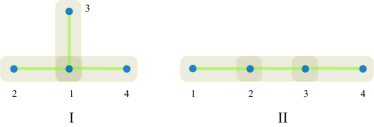
Figure 1: (color online). Two different configurations of monogamy relations. “Tree structure” (I) is for Eq. (28); and (II) as a “linked list” is for Eq. (29).

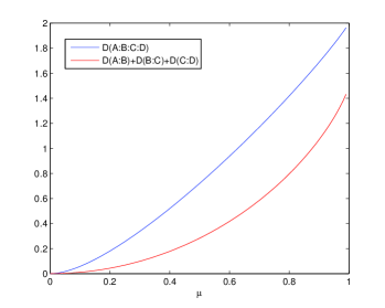
Figure 2: (color online). $D\left(A:B:C:D\right)$ and $D\left(A:B\right)+D\left(B:C\right)+D\left(C:D\right)$ v.s. $\mu$.

It is easy to show that these two monogamy relations are very different, not only in the physical meaning, but also in the structures of graph theory. A schematic description comparing these two monogamy relations is displayed in Fig. 1. From this figure, the standard monogamy relation relates to a “tree structure”, the second monogamy relation relates to a “linked list”. Therefore, these two monogamy relations are not equivalent. It’s worth noting that when we consider the quantum system which contains more parties, there will be more different structures for these two monogamy relations. The number of different structures increases very rapidly with growing $N$. This fact tells us that the monogamy structures of GQD are more than people have considered in the previous literature.

For instance, we consider a family of states as follows, $\rho={(1-\mu)}I^{\otimes N}/{2^{N}}+\mu|W(N)\rangle\langle W(N)|$, where $I$ is the identity and $\mu\in\left[0,1\right]$. Note that $|W(N)\rangle$ is the $N$-partite W state $(|10\cdots 0\rangle+|01\cdots 0\rangle+\cdots+|00\cdots 1\rangle)/{\sqrt{N}}$. In Fig. 2, $D\left(A:B:C:D\right)$ and $D\left(A:B\right)+D\left(B:C\right)+D\left(C:D\right)$ are plotted as a function of $\mu$. This figure shows that both two quantities increase as $\mu$ grows, $D\left(A:B:C:D\right)$ is always greater than or equal to the $D\left(A:B\right)+D\left(B:C\right)+D\left(C:D\right)$. Moreover, the difference between these two quantities first increases and then decreases as $\mu$ increases. That is to say, the non-nearest neighbor correlation first increases then decreases as the state becomes more closer to the $N$-partite W state with increasing $\mu$. For appropriate $\mu$, this non-nearest neighbor correlation reaches a maximum. It tells us that this correlation reaches a maximum for a part of mixed state, neither the completely mixed state nor the pure state. In fact, it is corresponding to the ”residual GQD” that we will considered in next section.

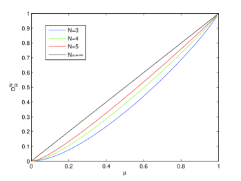
Figure 3: (color online). $D_{R}^{N}$ of Werner-GHZ state against $\mu$ for different $N$.

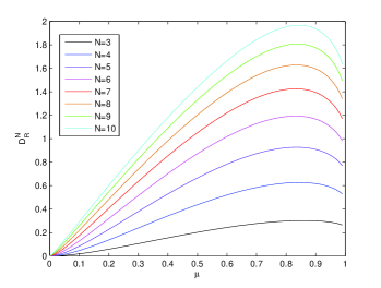
Figure 4: (color online). $D_{R}^{N}$ of mixed W state against $\mu$ for different $N$.

VI Residual GQD

Then, similar to the definition of tangle as a measure of residual multipartite entanglement, we can define the residual GQD corresponding to the second monogamy relation,

$$D_{R}^{N}\equiv D(A_{1}:\cdots:A_{N})-\sum_{K=1}^{N-1}D(A_{K}:A_{K+1}).$$ (30)

It is a measure for residual multipartite quantum correlations, namely, contributions to quantum correlations beyond pairwise GQD. This measure of residual multipartite quantum correlations describes the total quantum correlation except for all the nearest neighbor interaction of quantum correlations.

In order to better understand the residual GQD, let us consider two examples. First, we consider a $N$-qubit ($N\geq 2$) Werner-GHZ state key-29 , $\rho={(1-\mu)I^{\otimes N}}/{2^{N}}+\mu|\psi\rangle\langle\psi|$, where $|\psi\rangle$ is the $N$-qubit GHZ state $|\psi\rangle=\left(|00\ldots 0\rangle+|11\ldots 1\rangle\right)/{\sqrt{2}}$. In Fig. 3, the residual GQD $D_{R}^{N}$ of Werner-GHZ state is plotted as a function of $\mu$. From this figure, we can see that the residual GQD is always greater than or equal to zero. For more details, $D_{R}^{N}$ increases with an increasing $N$; when $N\rightarrow\infty$, $D_{R}^{N}$ approaches to the maximum value $\mu$. Furthermore, it is obvious that $D_{R}^{N}-D_{R}^{N-1}$ decreases with an increasing $N$; when $N\rightarrow\infty$, $D_{R}^{N}-D_{R}^{N-1}$ approaches to zero.

Next, we investigate the state considered in the former section, $\rho={(1-\mu)}I^{\otimes N}/{2^{N}}+\mu|W(N)\rangle\langle W(N)|$. In Fig. 4, the residual GQD:

$$D_{R}^{N} = \left[\left(N-1\right)\frac{1-\mu}{2^{N}}\log_{2}\left(\frac{1-\mu}{2^{N}}\right)-N\left(\frac{1-\mu}{2^{N}}+\frac{\mu}{N}\right)\log_{2}\left(\frac{1-\mu}{2^{N}}+\frac{\mu}{N}\right)+\left(\frac{1-\mu}{2^{N}}+{\mu}\right)\log_{2}\left(\frac{1-\mu}{2^{N}}+{\mu}\right)\right]$$ (31)

$$+ (N-1)\left[\left(\frac{1-\mu}{4}\right)\log_{2}\left(\frac{1-\mu}{4}\right)+\left(\frac{1-\mu}{4}+\frac{2\mu}{N}\right)\log_{2}\left(\frac{1-\mu}{4}+\frac{2\mu}{N}\right)-2\left(\frac{1-\mu}{4}+\frac{\mu}{N}\right)\log_{2}\left(\frac{1-\mu}{4}+\frac{\mu}{N}\right)\right]$$

is plotted as a function of $\mu$. This figure shows that the $D_{R}^{N}$ is always greater than or equal to zero for different $N$, so the second monogamy inequality always holds for this state. It’s worth noting that the $D_{R}^{N}$ always first increases and then decreases for different $N$, which is different from the behavior of the $N$-qubit Werner-GHZ state. Similar as the case in last section, the $D_{R}^{N}$ is always greater than or equal to $D_{R}^{N-1}$. For more details, it is obvious that when $N$ increases, the $D_{R}^{N}-D_{R}^{N-1}$ decreases. When $\mu\rightarrow 1$, $D_{R}^{N}$ is divergent for large $N$.

VII Global quantum discord and quantum phase transitions

It is known that quantum correlations such as entanglement amico ; key-30 ; key-31 ; key-32 ; fan1 ; fan2 , differential local convertibility p3 , non-locality key-33 and bipartite quantum discord key-34 can be applied to study the quantum phase transitions. The behavior of bipartite and global correlations in the quantum spin chains, especially for Ising model, has attracted considerable interest. Recently, it is worth noting that the behavior of global quantum discord of a finite-size transverse field Ising model near its critical point has been studied key-35 . Next, we also use Ising model with transverse filed as an example to show the application of the GQD. Let us consider a one dimensional Hamiltonian with periodic boundary conditions as follows:

$$\hat{H_{I}}=-J\sum_{i=1}^{L}\hat{\sigma}_{i}^{z}\hat{\sigma}_{i+1}^{z}+B\sum_{i=1}^{L}\hat{\sigma}_{i}^{x},$$ (32)

where we set the condition $L+1\equiv 1$. According to previous literature key-31 , in the limit $B/J\rightarrow 0$, the ground state of this model is locally equivalent to an $L$-spin GHZ state. As $B$ increases, in the thermodynamic limit, the system undergoes a quantum phase transition at $B/J=1$.

In this section, in line with key-35 , we will study (i) the total GQD for this $N$-partite spin system, (ii) sum of all the nearest neighbor bipartite GQDs, and (iii) the residual GQD as $B/J$ changes at $T=0$ and $T=0.1$. We will show that the sum of all the nearest neighbor bipartite GQDs is more effective and accurate for signaling the critical point of quantum phase transitions and the non-local correlations, such as residual GQD also plays an interesting role in this model.

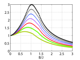
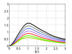
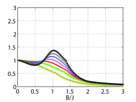
Figure 5: (color online). (a) GQD for the Ising model at zero temperature. From bottom to top curve, $L$ goes from $3$ to $9$ spins. At $B\rightarrow 0$ GQD =1 since the ground state is a GHZ state. In the paramagnetic configuration ( $B/J\gg 1$ ), GQD goes to zero. (b) The sum of all the nearest neighbor bipartite GQDs for the Ising model at zero temperature. From bottom to top curve, $L$ goes from $3$ to $9$ spins. At $B\rightarrow 0$, we have $\sum_{i=1}^{L-1}D\left(A_{i}:A_{i+1}\right)=0$. In the paramagnetic configuration ( $B/J\gg 1$ ), $\sum_{i=1}^{L-1}$ D $\left(A_{i}:A_{i+1}\right)$ goes to zero together with total GQD. (c) The residual GQD for the Ising model at zero temperature. From bottom to top curve, $L$ goes from $3$ to $9$ spins. At $B\rightarrow 0$ residual GQD equal to 1. In the region that $B/J\gg 1$, the residual GQD goes to zero faster than total GQD.

First, we consider the case of zero temperature. In order to calculate the global quantum correlations mentioned above, we first reformulate GQD as key-35 :

$$D(A_{1}:\cdots:A_{L}) = \underset{\{\hat{\Pi^{k}}\}}{\min}\left\{\sum_{j=1}^{L}\sum_{l=0}^{1}{\tilde{\rho}_{j}^{ll}}\log_{2}\tilde{\rho}_{j}^{ll}-\sum_{k=0}^{2^{L}-1}\tilde{\rho}_{T}^{kk}\log_{2}\tilde{\rho}_{T}^{kk}\right\}$$ (33)

$$+ \sum_{j=1}^{L}S(\rho_{j})-S(\rho_{T})$$

with $\tilde{\rho}_{T}^{kk}=\langle\bm{k}|\hat{{R}}^{{\dagger}}\rho_{T}\hat{{R}}|\bm{k}\rangle$ and $\tilde{\rho}_{j}^{ll}=\langle l|\hat{{R}}_{j}^{{\dagger}}\rho_{j}\hat{{R}}_{j}|l\rangle$, where $\hat{\Pi}^{k}=\hat{R}|\bm{k}\rangle\langle\bm{k}|\hat{R}^{{\dagger}}$ are the multi-qubit projective operators. Here $\left\{|\bm{k}\rangle\right\}$ are separable eigenstates of $\bigotimes_{j=1}^{L}\hat{\sigma}_{j}^{z}$, and $\hat{R}$ is a local $L$-qubit rotation: $\hat{R}=\bigotimes_{j=1}^{L}\hat{R}_{j}(\theta_{j},\phi_{j})$ with $\hat{R_{j}}(\theta_{j},\phi_{j})=\cos\theta_{j}\hat{I}+i\sin\theta_{j}\cos\phi_{j}\hat{\sigma}_{y}+i\sin\theta_{j}\sin\phi_{j}\hat{\sigma}_{x}$ acting on the $j$-th qubit. Considering the symmetries of this model, the GQD is completely independent on the set of $\phi_{j}$ angles, so we only need to optimize the $\theta_{j}$. Similar as the literature key-35 , the optimal $\theta_{j}$ all take the same value $\bar{\theta}$, which depends on the magnetic field.

Fig. 5 shows the GQD as a function of the ratio $B/J$ between the magnetic field intensity and the Ising interaction constant when $T=0$. We study rings with $L=3,\ldots,9$. GQD curves share the same value $1$ as $B\rightarrow 0$, since the ground state of our model is an $L$-spin GHZ state. When $B/J$ tends to $1$, the GQD increases reaching a maximum at different positions depending on size $L$ of the system. In the paramagnetic phase achieved for $B/J\gg 1$, all the spins align along the direction of the magnetic field, so that global discord disappears. We find that the height and position of the maximum of GQD is varies in accordance with the system size $L$.

Fig. 5 shows the sum of all the nearest neighbor bipartite GQDs: $D\left(A_{1}:A_{2}\right)+D\left(A_{2}:A_{3}\right)+\cdots+D\left(A_{L-1}:A_{L}\right)$ as a function of the ratio $B/J$ when $T=0$. We still study rings with $L=3,\ldots,9$, whose curves share the same value $0$ at $B\rightarrow 0$. As $B/J$ tends to $1$, $\sum_{i=1}^{L-1}D\left(A_{i}:A_{i+1}\right)$ reaches a maximum at nearly $B/J=1$, which almost independent on the size of the system. It shows that the behavior of the sum of all the nearest neighbor bipartite GQDs is quite different with total GQD, and is more suited to be used to describe the quantum phase transitions in this model. It is because that our Hamiltonian only contains the nearest-neighbor interactions. In the region that $B/J\gg 1$, similar as the total GQD, the sum of all the nearest neighbor bipartite GQDs also disappears.

Fig. 5 shows the residual GQD: $D_{R}^{L}$ (see Eq. (30)) as a function of the ratio $B/J$ when $T=0$. We still study rings with $L=3,\ldots,9$, whose residual GQD curves share the same value $1$ at $B\rightarrow 0$ since the sum of all the nearest neighbor bipartite GQDs disappears at this point. The behavior of residual GQD is very sensitive to the system’s size $L$. For $L=3,4$, the residual GQD is monotonically decreasing. When the system’s size $L$ increases, the residual GQD is not monotonous. As $B/J$ is around $1$, it can also be used to characterize the quantum phase transitions in this model when we consider the appropriate system’s size $L$. This fact tells us that for the large system, the non-nearest-neighbor correlations also play an important role in the quantum phase transitions although our Hamiltonian only contains the nearest neighbor interactions. This phenomenon reflects that the nearest neighbor interactions can also create long-range correlations. In the region that $B/J\gg 1$, the residual GQD tends to $0$ faster than the sum of all the nearest neighbor bipartite GQDs. It shows that when we consider the large magnetic field, the long-range correlations disappear firstly.

Comparing these three figures in Fig. 5, we find that the sum of all the nearest neighbor bipartite GQDs gives the best criteria for the critical point of the quantum phase transitions. Since the total GQD is the sum of residual GQD together with the sum of all the nearest neighbor bipartite GQDs, the shift of the maximum point of total GQD away from the critical point may be due to the shift of the maximum of residual GQD.

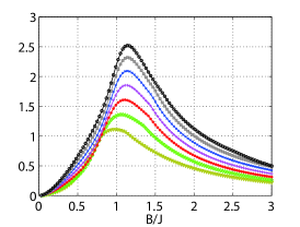
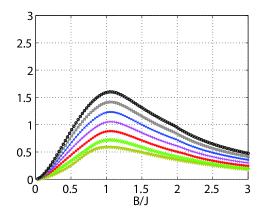
Figure 6: (color online). (a) GQD for the Ising rings containing from $3$ to $9$ spins at $T=0.1$. GQD is null at zero magnetic field. For increasing temperatures the maximum values of the curves decrease. (b) The sum of all the nearest neighbor bipartite GQDs for the Ising rings containing from $3$ to $9$ spins at $T=0.1$. $\sum_{i=1}^{L-1}$ D $\left(A_{i}:A_{i+1}\right)$ is null at $B=0$. In the region that $B/J\gg 1$, $\sum_{i=1}^{L-1}$ D $\left(A_{i}:A_{i+1}\right)$ goes to zero together with total GQD.

Next, we consider the case that $T\neq 0$. Similar as key-35 , we take the Gibbs state as our thermal state:

$$\rho_{T}=\frac{e^{-\hat{H}/T}}{\mathcal{Z}}$$ (34)

with $\hat{H}_{I}$ the Hamiltonian describing the interaction, $T$ the effective temperature, and $\mathcal{Z}=\textrm{Tr}[\exp({-\hat{H}_{I}/T})]$ the partition function.

We consider the behavior of total GQD and the sum of all the nearest neighbor bipartite GQDs with effective temperature $T=0.1$ in Fig. 6 and Fig. 6, respectively. Fig. 6 shows the GQD as a function of the ratio $B/J$ when $T=0.1$. It’s worth noting that at non-zero temperature, the quantum correlations presented in the ground state at $B=0$ are destroyed since as $B\rightarrow 0$ the ground and first excited states approach degeneracy. It is obvious that the height of the curves decreases with increasing temperature and there is a right shift in the maxima of each curve.

Fig. 6 shows the sum of all the nearest neighbor bipartite GQDs as a function of the ratio $B/J$ when $T=0.1$. Comparing Fig. 6 with Fig. 5, it is amazing that the behavior of $\sum_{i=1}^{L-1}D\left(A_{i}:A_{i+1}\right)$ is almost independent of the effective temperature $T$. That is to say, the sum of all the nearest neighbor bipartite GQDs is more suited to be used to describe the quantum phase transition in our model both for zero temperature and non-zero effective temperature. We remark that the residual GQD can be negative for non-zero temperature, so it is no longer a well-defined quantum correlation in this case. This fact reflects that at non-zero temperature the non-nearest-neighbor correlations are destroyed.

VIII conclusions and discussion

In summary, we have introduced a series of generalized monogamy relations of GQD for an $N$-partite system. Remarkably, these monogamy relations hold for general states whose bipartite GQDs is non-increasing in discarding of subsystems. Using the decomposition property of GQD, we provide a family of monogamy inequalities which can be considered as an extension of the standard monogamy inequality. We have proved that they hold under the similar condition as that for standard monogamy relation and shown that there is an intrinsic connection between them. We also demonstrate that GQD of an $N$-partite system is not less than the sum of GQDs of its subsystems plus GQD between all its subsystems under any decomposition. Furthermore, we have provided the second class of monogamy inequality which is also upper bounded by GQD of a multipartite system. It reflects how GQD is distributed in the multipartite quantum system from a new aspect. In particular, when $K=1$, one of the special case of the second class of monogamy inequality is obtained and shows that the GQD of an $N$-partite system is greater than or equal to the sum of GQDs between two nearest neighbor particles. Its physical meaning is quite different from the standard monogamy relation. Last but not least, we provide the residual GQD corresponding to the second monogamy inequality and study its properties by considering two typical states.

More importantly, we demonstrate an interesting application of the sum of all the nearest neighbor bipartite GQDs and residual GQD . By considering their behavior in the transverse field Ising model, we find that both of them can be used to characterize the quantum phase transitions at zero temperature. It is worth noting that the sum of all the nearest neighbor bipartite GQDs is more suited to be used to describe the quantum phase transition in our model both for zero temperature and non-zero effective temperature case. This result is superior to the the results obtained in the previous literature key-35 . That is to say, we provide a new and more effective way to characterize the quantum phase transitions in this model.

We believe that our result provide a useful method in understanding the distribution property of GQD in multipartite quantum systems. The introduced quantities not only play a fundamental role in the quantum information processing, but also can be applied to physical models of many-body quantum systems.

APPENDIX

A1. Proof of Theorem 1

Proof.

In order to simplify our proof, we first consider a special case as follows:

$$D(A_{1}:\cdots:A_{N})\geq D(A_{1}:A_{2}:\cdots:A_{m})+D(A_{1}:A_{m+1}:\cdots:A_{N}).$$ (A1-1)

According to the definition of GQD, we have $D(A_{1}:\cdots:A_{N})=\underset{\Phi}{\min}D_{\Phi}(A_{1}:\cdots:A_{N})$. Using property $\left(a\right)$, we can rewrite $D_{\Phi}(A_{1}:\cdots:A_{N})$ as following form:

$$D_{\Phi}(A_{1}:\cdots:A_{N}) = \sum_{k=1}^{N-1}D_{\Phi}\left(A_{1}\cdots A_{k}:A_{k+1}\right)=\sum_{k=1}^{m-1}D_{\Phi}\left(A_{1}\cdots A_{k}:A_{k+1}\right)+\sum_{k=m}^{N-1}D_{\Phi}\left(A_{1}\cdots A_{k}:A_{k+1}\right)$$ (A1-2)

$$= D_{\Phi}(A_{1}:\cdots:A_{m})+\sum_{k=m}^{N-1}D_{\Phi}\left(A_{1}\cdots A_{k}:A_{k+1}\right).$$

Thus, we have

$$D_{\Phi}(A_{1}:\cdots:A_{N})-D_{\Phi}(A_{1}:\cdots:A_{m})=\sum_{k=m}^{N-1}D_{\Phi}\left(A_{1}\cdots A_{k}:A_{k+1}\right).$$ (A1-3)

Similarly we can rewrite $D_{\Phi}(A_{1}:A_{m+1}:\cdots:A_{N})$ :

$$D_{\Phi}(A_{1}:A_{m+1}:\cdots:A_{N})=D_{\Phi}(A_{1}:A_{m+1})+D_{\Phi}(A_{1}A_{m+1}:A_{m+2})+\cdots+D_{\Phi}(A_{1}A_{m+1}\cdots A_{N-1}:A_{N}).\ \ \ \$$ (A1-4)

Now we have

$$D_{\Phi}(A_{1}:\cdots:A_{N})-D_{\Phi}(A_{1}:\cdots:A_{m})-D_{\Phi}(A_{1}:A_{m+1}:\cdots:A_{N})$$ (A1-5)

$$= \sum_{k=m}^{N-1}D_{\Phi}\left(A_{1}\cdots A_{k}:A_{k+1}\right)-[D_{\Phi}(A_{1}:A_{m+1})+D_{\Phi}(A_{1}A_{m+1}:A_{m+2})+\cdots+D_{\Phi}(A_{1}A_{m+1}\cdots A_{N-1}:A_{N})]$$

$$= [D_{\Phi}\left(A_{1}\cdots A_{m}:A_{m+1}\right)-D_{\Phi}(A_{1}:A_{m+1})]+\cdots+[D_{\Phi}\left(A_{1}A_{m+1}:A_{m+2}\right)-D_{\Phi}(A_{1}A_{m+1}:A_{m+2})]+\cdots$$

$$+ [D_{\Phi}\left(A_{1}\cdots A_{N-1}:A_{N}\right)-D_{\Phi}(A_{1}A_{m+1}\cdots A_{N-1}:A_{N})].$$

We first minimize both sides of this equation with respect to $\Phi\left(\rho_{A_{1}\cdots A_{N}}\right)$. Since we have that the bipartite GQDs do not increase under the discard of subsystems and every item of the right hand side is greater than or equal to zero, it is obvious that

$$\underset{\Phi}{\min}D_{\Phi}(A_{1}:\cdots:A_{N}) \geq \underset{\Phi}{\min}D_{\Phi}(A_{1}:A_{2}:\cdots:A_{m})+\underset{\Phi}{\min}D_{\Phi}(A_{1}:A_{m+1}:\cdots:A_{N})$$ (A1-6)

$$\Rightarrow D(A_{1}:\cdots:A_{N}) \geq D(A_{1}:A_{2}:\cdots:A_{m})+D(A_{1}:A_{m+1}:\cdots:A_{N}).$$ (A1-7)

Similarly, by using the condition that the bipartite GQDs do not increase under the discard of subsystems, we can prove the general form of these monogamy inequalities. ∎

A2. Proof of Theorem 2

Proof.

In order to simplify our proof, we first consider a special case as follows:

$$D_{\Phi}(A_{1}:\cdots:A_{N})=D_{\Phi}(A_{1}:\cdots:A_{K})+D_{\Phi}(A_{K+1}:\cdots:A_{N})+D_{\Phi}(A_{1}\cdots A_{K}:A_{K+1}\cdots A_{N}).$$ (A2-1)

According to the definition of GQD, we have $D(A_{1}:\cdots:A_{N})=\underset{\Phi}{\min}D_{\Phi}(A_{1}:\cdots:A_{N})$, so we only need to consider the relationship between $D_{\Phi}$. Using the definition, the $D_{\Phi}$ can be rewritten as follows:

$$D_{\Phi}(A_{1}:\cdots:A_{N})=I\left(\rho_{A_{1}\cdots A_{N}}\right)-I\left(\Phi\left(\rho_{A_{1}\cdots A_{N}}\right)\right).$$ (A2-2)

Noting that the $I\left(\rho_{A_{1}\cdots A_{N}}\right)$ and $I\left(\Phi(\rho_{A_{1}\cdots A_{N}})\right)$ can be decomposed as

$$I\left(\rho_{A_{1}\cdots A_{N}}\right) = I\left(\rho_{A_{1}\cdots A_{K}}\right)+I\left(\rho_{A_{K+1}\cdots A_{N}}\right)+I\left(\rho_{\left(A_{1}\cdots A_{K}\right)\left(A_{K+1}\cdots A_{N}\right)}\right)$$ (A2-3)

$$I\left(\Phi(\rho_{A_{1}\cdots A_{N}})\right) = I\left(\Phi(\rho_{A_{1}\cdots A_{K}})\right)+I\left(\Phi(\rho_{A_{K+1}\cdots A_{N}})\right)+I\left(\Phi(\rho_{\left(A_{1}\cdots A_{K}\right)\left(A_{K+1}\cdots A_{N}\right)})\right).$$ (A2-4)

Thus, this particular case has been proved.

Furthermore, we can prove the general form of this identity by using the similar decomposition of $I\left(\rho_{A_{1}\cdots A_{N}}\right)$ as follows:

$$I\left(\rho_{A_{1}\cdots A_{N}}\right)=I\left(\rho_{A_{1}\cdots A_{K_{1}}}\right)+\cdots+I\left(\rho_{A_{K_{N}+1}\cdots A_{N}}\right)+I\left(\rho_{\left(A_{1}\cdots A_{K_{1}}\right)\cdots\left(A_{K_{N}+1}\cdots A_{N}\right)}\right),$$ (A2-5)

which completes the proof. ∎

A3. Proof of Proposition 1

Proof.

In order to prove the above inequality, first of all, we use $D_{T}$, $D_{K_{1}}$, $D_{K_{2}}$, $D_{K_{3}}$, $\cdots$ , $D_{N}$ and $D_{I}$ to represent $D(A_{1}:\cdots:A_{N})$, $D(A_{1}:\cdots:A_{K_{1}})$, $D(A_{K_{1}+1}:\cdots:A_{K_{2}})$, $D(A_{K_{2}+1}:\cdots:A_{K_{3}})$, $\cdots$, $D(A_{K_{N}+1}:\cdots:A_{N})$, $D(A_{1}\cdots A_{K_{1}}:A_{K_{1}+1}\cdots A_{K_{2}}:A_{K_{2}+1}\cdots A_{K_{3}}:\cdots:A_{K_{N}+1}\cdots A_{N})$. Now we need to show that

$$[D_{T}]^{n}\geq[D_{K_{1}}]^{n}+[D_{K_{2}}]^{n}+[D_{K_{3}}]^{n}+\cdots+[D_{N}]^{n}+[D_{I}]^{n}.$$ (A3-1)

According to the above Theorem 2, we have

$$[D_{T}]^{n}\geq[(D_{K_{1}}+D_{K_{2}}+D_{K_{3}}+\cdots+D_{N})+D_{I}]^{n}.$$ (A3-2)

Using the binomial theorem, the above formula can be re-expressed as

$$[D_{T}]^{n}\geq\sum_{k=0}^{n}C_{n}^{k}(D_{K_{1}}+D_{K_{2}}+D_{K_{3}}+\cdots+D_{N})^{n-k}D_{I}^{k}=(D_{K_{1}}+D_{K_{2}}+D_{K_{3}}+\cdots+D_{N})^{n}+D_{I}^{n}$$

$$+\sum_{k=1}^{n-1}C_{n}^{k}(D_{K_{1}}+D_{K_{2}}+D_{K_{3}}+\cdots+D_{N})^{n-k}D_{I}^{k}\geq(D_{K_{1}}+D_{K_{2}}+D_{K_{3}}+\cdots+D_{N})^{n}+D_{I}^{n}.$$ (A3-3)

Similarly, by using the same procedure many times, we have

$$[D_{T}]^{n}\geq(D_{K_{1}}+D_{K_{2}}+D_{K_{3}}+\cdots+D_{N})^{n}+D_{I}^{n}\geq(D_{K_{1}}+D_{K_{2}}+D_{K_{3}}+\cdots+D_{K_{N}})^{n}+D_{N}^{n}+D_{I}^{n}$$

$$\cdots\ \ \ \ \ \ \ \ \ \ \ \ \ \ \ \ \ \ \$$

$$\geq(D_{K_{1}}+D_{K_{2}})^{n}+D_{K_{3}}^{n}+\cdots+D_{N}^{n}+D_{I}^{n}\geq[D_{K_{1}}]^{n}+[D_{K_{2}}]^{n}+[D_{K_{3}}]^{n}+\cdots+[D_{N}]^{n}+[D_{I}]^{n},$$ (A3-4)

which completes the proof. ∎

A4. Proof of Theorem 3

Proof.

In order to prove the above inequality, we only need to consider the relationship between $D_{\Phi}$. By using property $\left(a\right)$, $D_{\Phi}\left(A_{1}:\cdots:A_{N}\right)$ can be decomposed as follows:

$$D_{\Phi}(A_{1}:\cdots:A_{N}) = D_{\Phi}(A_{1}:A_{2}:\cdots:A_{K})+D_{\Phi}(A_{1}\cdots A_{K}:A_{K+1})+D_{\Phi}(A_{1}\cdots A_{K+1}:A_{K+2})+\cdots+D_{\Phi}(A_{1}\cdots A_{N-1}:A_{N})$$ (A4-1)

$$= D_{\Phi}(A_{1}:A_{2}:\cdots:A_{K})+\sum_{j=K}^{N-1}D_{\Phi}(A_{1}\cdots A_{j}:A_{j+1}).\ \ \ \ \ \ \ \$$

Then we have

$$D_{\Phi}(A_{1}:\cdots:A_{N})-\sum_{i=1}^{N-K}D_{\Phi}(A_{i}\cdots A_{i+K-1}:A_{i+K}) = D_{\Phi}(A_{1}:A_{2}:\cdots:A_{K})+[D_{\Phi}(A_{1}\cdots A_{K+1}:A_{K+2})-D_{\Phi}(A_{2}\cdots A_{K+1}:A_{K+2})]$$ (A4-2)

$$+ \cdots+[D_{\Phi}(A_{1}\cdots A_{N-1}:A_{N})-D_{\Phi}(A_{N-K}\cdots A_{N-1}:A_{N})].$$

After minimizing both sides of this equation with respect to $\Phi\left(\rho_{A_{1}\cdots A_{N}}\right)$, we have that the bipartite GQDs do not increase under the discard of subsystems and every item of the right hand side is greater than or equal to zero. We therefore have

$$D(A_{1}:\cdots:A_{N})-\sum_{i=1}^{N-K}D(A_{i}\cdots A_{i+K-1}:A_{i+K})\geq D(A_{1}:A_{2}:\cdots:A_{K})\geq 0,$$ (A4-3)

which completes the proof. ∎

References

- (1) C. H. Bennett et al., Phys. Rev. Lett. 70, 1895 (1993).
- (2) A. K. Ekert, Phys. Rev. Lett. 67, 661 (1991).
- (3) C. H. Bennett, Phys. Rev. Lett. 68, 3121 (1992).
- (4) M. Gu et al., Nature Phys. 8, 671 (2012).
- (5) R. Horodecki, P. Horodecki, and M. Horodecki, Rev. Mod. Phys. 81, 865 (2009).
- (6) K. Modi, A. Brodutch, H. Cable, T. Paterek, and V. Vedral, Rev. Mod. Phys. 84, 1655 (2012).
- (7) B. Dakic, Y. O. Lipp, and X. S. Ma, Nature Phys. 8, 666 (2012).
- (8) L. Amico, R. Fazio, A. Osterloh, and V. Vedral, Rev. Mod. Phys. 80, 517 (2008).
- (9) A. Osterloh, L. Amico, G. Falci, and R. Fazio, Nature 418, 608 (2002).
- (10) J. Cui, M. Gu, L. C. Kwek, M. F. Santos, H. Fan, and V. Vedral, Nature Commun. 3, 812 (2012).
- (11) Z. Liu, E. J. Bergholtz, H. Fan, and A. M. Lauchli, Phys. Rev. Lett. 109, 186805 (2012).
- (12) H. Fan, V. Korepin and V. Roychowdhury, Phys. Rev. Lett. 93, 227203 (2004).
- (13) E. Knill and R. Laflamme, Phys. Rev. Lett. 81, 5672 (1998).
- (14) A. Datta, S. T. Flammia and C. M. Caves, Phys. Rev. A 72, 042316 (2005).
- (15) A. Datta and G. Vidal, Phys. Rev. A 75, 042310 (2007).
- (16) H. Ollivier and W. H. Zurek, Phys. Rev. Lett. 88, 017901 (2001).
- (17) L. Henderson and V. Vedral, J. Phys. A. 34, 6899 (2001).
- (18) R. Dillenschneider, Phys. Rev. B 78, 224413 (2008); M. S. Sarandy, Phys. Rev. A 80, 022108 (2009).
- (19) T. Werlang et al., Phys. Rev. Lett. 105, 095702 (2010).
- (20) J. Maziero et al., Phys. Rev. A 82, 012106 (2010)
- (21) Y.-X. Chen and S.-W. Li, Phys. Rev. A 81, 032120 (2010).
- (22) A. Shabani and D. A. Lidar, Phys. Rev. Lett. 102, 100402 (2009); J. Maziero et al., Phys. Rev. A 80, 044102 (2009).
- (23) J. Maziero et al., Phys. Rev. A 81, 022116 (2010); A. Ferraro et al., Phys. Rev. A 81, 052318 (2010); L. Mazzola, J. Piilo, and S. Maniscalco, Phys. Rev. Lett. 104, 200401 (2010).
- (24) A. Datta, A. Shaji, and C.M. Caves, Phys. Rev. Lett. 100, 050502 (2008).
- (25) C. C. Rulli and M. S. Sarandy, Phys. Rev. A 84, 042109 (2011); M. Okrasa and Z. Walczak, Eur. Phys. Lett. 96, 60003 (2011).
- (26) K. Modi et al., Phys. Rev. Lett. 104, 080501 (2010).
- (27) I. Chakrabarty, P. Agrawal and A. K. Pati, Eur. Phys. J. D. 65, 605 (2011).
- (28) L. Chen, E. Chitambar, K. Modi, and G. Vacanti, Phys. Rev. A 83, 020101(R) (2011).
- (29) V. Coffman, J. Kundu, and W. K. Wootters, Phys. Rev. A 61, 052306 (2000).
- (30) R. Prabhu, A. K. Pati, A. Sen(De), and U. Sen, Phys. Rev. A 85, 040102(R) (2012).
- (31) G. L. Giorgi, Phys. Rev. A 84, 054301 (2011).
- (32) H. C. Braga et al., Phys. Rev. A 86, 062106 (2012).
- (33) S. Campbell, L. Mazzola, and M. Paternostro, Int. J. Quantum Inf. 9, 1685 (2011).
- (34) M. Piani, P. Horodecki, and R. Horodecki, Phys. Rev. Lett. 100, 090502 (2008).
- (35) S.-Y. Liu, B. Li, W.-L. Yang, and H. Fan, Phys. Rev. A 87, 062120 (2013).
- (36) J.-W. Xu, Phys. Lett. A 377, 238 (2013).
- (37) T. J. Osborne and M. A. Nielsen, Phys. Rev. A 66, 032110 (2002).
- (38) A. Osterloh, L. Amico, G. Falci, and R. Fazio, Nature 416 608 (2002).
- (39) P. Štelmachovič and V. Bužek, Phys. Rev. A 70, 032313 (2004).
- (40) F. Igloi and Y. C. Lin, J. Stat. Mech. P06004, (2008); F. Iglói and R. Juhász, Eur. Phys. Lett. 81, 57003 (2008).
- (41) Z. Liu, E. J. Bergholtz, H. Fan and A. M. Lauchli, Phys. Rev. Lett. 109, 186805 (2012).
- (42) D. Wang, Z. Liu, J. P. Cao, and H. Fan, Phys. Rev. Lett. 111, 186804 (2013).
- (43) S. Campbell and M. Paternostro, Phys. Rev. A 82, 042324 (2010).
- (44) S. Campbell, L. Mazzola and M. Paternostro, Int. J. Quant. Inf. 9, 1685 (2011).
- (45) S. Campbell, L. Mazzola, G. De Chiara, T. J. G. Apollaro, F. Plastina, Th. Busch and M. Paternostro, New J. Phys. 15, 043033 (2013).