Dynamical transition in the $D=3$ Edwards-Anderson spin glass in an external magnetic field

Abstract

We study the off-equilibrium dynamics of the three-dimensional Ising spin glass in the presence of an external magnetic field. We have performed simulations both at fixed temperature and with an annealing protocol. Thanks to the Janus special-purpose computer, based on FPGAs, we have been able to reach times equivalent to $0.01$ seconds in experiments. We have studied the system relaxation both for high and for low temperatures, clearly identifying a dynamical transition point. This dynamical temperature is strictly positive and depends on the external applied magnetic field. We discuss different possibilities for the underlying physics, which include a thermodynamical spin-glass transition, a mode-coupling crossover or an interpretation reminiscent of the random first-order picture of structural glasses.

I Introduction

The glass transition is a ubiquitous but still mysterious phenomenon in condensed matter physics Debenedetti (1997); Debenedetti and Stillinger (2001); Cavagna (2009). Indeed, many materials display a dramatic increase in their relaxation times when cooled down to their glass temperature $T_{\mathrm{g}}$. Examples include fragile molecular glasses, polymers, colloids or, more relevant here, disordered magnetic alloys named spin glasses Mydosh (1993). The dynamic slowing down is not accompanied by dramatic changes in structural or thermodynamic properties. In spite of this, quite general arguments suggest that the sluggish dynamics must be correlated with an increasing length scale Montanari and Semerjian (2006). This putative length scale can be fairly difficult to identify (a significant amount of research has been devoted to this problem, see, e.g., Adam and Gibbs (1965); Weeks et al. (2000); Berthier et al. (2005)).

In this context, spin glasses are unique for a number of reasons. To start with, they provide the only example of a material for which it is widely accepted that the sluggish dynamics is due to a thermodynamic phase transition at a critical temperature $T_{\text{c}}=T_{\mathrm{g}}$ Gunnarsson et al. (1991); Palassini and Caracciolo (1999); Ballesteros et al. (2000). This phase transition is continuous, and the time-reversal symmetry of the system is spontaneously broken at $T_{\text{c}}$.

Spin glasses are also remarkable because special tools are available for their investigation. On the experimental side, time-dependent magnetic fields are a very flexible tool to probe their dynamic response, which can be very accurately measured with a SQUID (for instance, see Hérisson and Ocio (2002)). For very low applied magnetic fields, one can measure glassy magnetic domains of a diameter up to $\xi\sim 100$ lattice spacings Joh et al. (1999); Bert et al. (2004), much larger than any length scale identified for structural glasses Berthier et al. (2005). On the theoretical side, spin glasses are simple to model, which greatly eases numerical simulation. In fact, special-purpose computers have been built for the simulation of spin glasses Cruz et al. (2001); Ogielski (1985); Belletti et al. (2006, 2008a, 2008b). In particular, the Janus computer Belletti et al. (2006, 2008a) has allowed us to simulate the non-equilibrium dynamics from picoseconds to a tenth of a second Belletti et al. (2008b, 2009a), which has resulted in detailed connections between non-equilibrium dynamics at finite times and equilibrium physics in finite systems Alvarez Baños et al. (2010a, b) (see also Franz et al. (1998)).

Now, Mean Field provides compelling motivation to investigate spin glasses in an externally applied magnetic field. Although a magnetic field explicitly breaks time-reversal symmetry, it has been shown that a phase transition should still occur when cooling the mean-field spin glass in an external field de Almeida and Thouless (1978); Mézard et al. (1987); Marinari et al. (2000), which leads us to expect a sophisticated and still largely unexplored behavior for short-range spin glasses. In this respect, we remark as well an intriguing suggestion by Moore, Drossel and Fullerton. These authors speculate that the spin glass in a field sets the universality class for the structural-glass transition Moore and Drossel (2002); Fullerton and Moore (2013) (the statement is supposed to hold in $d=3$ spatial dimensions; spatial dimensionality is crucial).

However, two major problems hamper further progress: (i) the mean-field theory, which is expected to be accurate above the upper critical dimension $d>d_{\text{u}}=6$, predicts a rather different behavior for spin and structural glasses; (ii) the behavior of spin glasses in a field in $d=3$ is the matter of a lively controversy. We now address each issue separately.

Regarding the first problem, we note that the standard mean-field model for structural glasses is the $p$-spin glass model, with $p$-body interactions Kirkpatrick and Thirumalai (1987); Kirkpatrick et al. (1989) (for odd $p$, the time-reversal symmetry is explicitly broken). In the mean-field approximation, the odd-$p$ models display a dynamic phase transition in their paramagnetic phase. Reaching thermal equilibrium becomes impossible in the temperature range $T_{\mathrm{c}}<T<T_{\text{g}}$. The dynamic transition at $T_{\text{g}}$ is identical to the ideal Mode Coupling transition of supercooled liquids Götze and Sjögren (1992). The thermodynamic phase transition at $T_{\mathrm{c}}$ is analogous to the ideal Kauzmann thermodynamic glass transition Cavagna (2009). The thermodynamic transition is very peculiar: although it is of the second order (in the Ehrenfest sense), the spin-glass order parameter jumps discontinuously at $T_{\mathrm{c}}$ from zero to a non-vanishing value. On the other hand, for spin glasses in a field, mean-field theory predicts a single transition (i.e., $T_{\mathrm{c}}=T_{\text{g}}$) and an order parameter that behaves continuously as a function of temperature.

However, mean-field theory is accurate only in high-enough spatial dimensions, $d>d_{\text{u}}=6$, hence it is legitimate to wonder about our three-dimensional world. In fact, the ideal Mode Coupling transition is known to be only a crossover for supercooled liquids. The power-law divergences predicted by Mode Coupling theory hold when the equilibration time lies in the range $10^{-13}\text{ s}<\tau<10^{-5}\text{ s}$. Fitting to those power-laws, one obtains a Mode Coupling temperature $T_{\mathrm{MC}}$. However, $\tau$ is finite at $T_{\mathrm{MC}}$ (typically $T_{\mathrm{MC}}$ is 10% larger than the glass temperature $T_{\text{g}}$ where $\tau\sim 10^{4}$ seconds). A theory for a thermodynamic glass transition at $T_{\mathrm{c}}<T_{\text{g}}$ has been put forward Mézard and Parisi (1999a, b); Coluzzi et al. (2000); Parisi and Rizzo (2010), but it has still not been validated (however, see Singh et al. (2013)).

Regarding now our second problem, we recall that whether spin glasses in a magnetic field undergo a phase transition has been a long-debated and still open question. There are mainly two conflicting theories. The above mentioned mean-field picture is the replica symmetry breaking (RSB) theory Mézard et al. (1987). On the other hand, the droplet theory McMillan (1984); Bray and Moore (1987); Fisher and Huse (1986, 1988) predicts that the system’s behavior is akin to that of a disguised ferromagnet (i.e., no phase transition in a field). Recent exponents of this controversy are Moore and Bray (2011); Parisi and Temesvári (2012); Yeo and Moore (2012). We elaborate on concrete predictions by both theories in Section II.3. For now, we note that recent numerical simulations in $d=3$ did not find the thermodynamic transition predicted by mean-field Young and Katzgraber (2004); Jörg et al. (2008). Experimental studies have been conducted as well, with conflicting conclusions Jönsson et al. (2005); Petit et al. (1999, 2002); Tabata et al. (2010). Up to now, a transition has been found only numerically, in four dimensions (note that $4<d_{\mathrm{u}}=6$) Baños et al. (2012).

A different numerical approach has consisted in the study of Levy graphs: one-dimensional systems where the interaction decays with distance as a power-law $J(r)\sim 1/r^{\hat{a}}$ Kotliar et al. (1983). It has been suggested that the critical behavior in $d$ spatial dimensions can be matched with that of a Levy graph with an appropriate choice of the decay exponent $\hat{a}$. The spin-glass transition has been investigated in this way, both with and without an externally applied magnetic field. The latest result within this approach suggests that the de Almeida-Thouless line is present in four spatial dimensions, but not in three dimensions Larson et al. (2013). However, it has been pointed out that the matching between the decay exponent $\hat{a}$ and the spatial dimension $d$ changes when a magnetic field is applied Leuzzi and Parisi (2013), a possibility not considered in Larson et al. (2013).

Our scope here is to explore the dynamical behavior of $d=3$ spin glasses in a field using the Janus computer. We shall study lattices of size $L=80$, where we expect finite-size effects to be negligible Belletti et al. (2008b). Our time scales will range from 1 picosecond (i.e., one Monte Carlo full lattice sweep Mydosh (1993)) to $0.01$ seconds. Hence, if the analogy with structural glasses holds, we should be able to identify the Mode Coupling crossover. Our study will be eased by the rather deep theoretical knowledge of the relevant correlation functions de Dominicis and Giardina (2006). Hence, we shall be able to correlate the equilibration time $\tau$ with the correlation length $\xi$.

The layout of the remaining part of this work is as follows. In Section II we describe the model and our observables and we give an overview of the different theoretical pictures that have been put forward to explain the dynamics of the spin glass in a field. We pay particular attention to the specific predictions for the observables that we are going to study (Sections II.3 and Section II.4). In Section III we describe the different protocols that we have considered (simulating a direct quench and annealings with different temperature variation rates). Next, in Section III.2, we turn our attention to the crucial and delicate issue of identifying intrinsic time scales in the dynamics.

Once this foundation has been laid, we delve into the physical analysis and interpretation of our results. First, we consider the high-temperature regime, where our simulations reach equilibrium, in Section IV. We thus try to approach the critical region from above. Afterwards, in Section V, we study the low-temperature regime, where the relaxation times are much longer than our simulations (perhaps infinite). We consider two complementary approaches: in Section V.1 we try the simplest ansatz for a low-temperature behavior compatible with a RSB spin-glass transition, while in Section V.2 we assume from the outset that no transition occurs. The spatial correlation of the system is studied in Section VI, where we carry out a direct analysis of the correlation length. Finally, in Section VII we present our conclusions, evaluating the different physical scenarios on the light of our data.

We also include two appendices: one describing some details of our implementation and the other presenting a more detailed look at the correlation functions.

II Model, observables and the droplet-RSB controversy

In Section II.1 we describe the model that we have simulated. The observables that we consider are defined in Section II.2. At that point, we will be ready to describe the different predictions of the droplet and RSB theories in Section II.3. However, it has been recently suggested that spin-glass on a field behave just as supercooled liquids Moore and Drossel (2002); Fullerton and Moore (2013). The current theoretical predictions for supercooled liquids do not quite match neither the droplet nor the RSB theories for spin glasses on a field. Hence, we briefly recall those predictions in Section II.4.

II.1 Model

We have studied a three-dimensional cubic lattice system with volume $V=L^{3}$ ($L$ is the linear size) and periodic boundary conditions. On every node of the lattice there is an Ising spin $\sigma{x}$ and nearest neighbors are joined by couplings $J{xy}$. The spins are dynamic variables, while the couplings $J{xy}$ are fixed during the simulation (this is the so-called quenched disorder Parisi (1994)). The couplings are independent random variables: $J{xy}=\pm 1$ with $50\%$ probability. We also include a local magnetic field $h{x}$ on every node. The magnetic field is Gaussianly distributed with zero mean and variance $H^{2}$. The Hamiltonian of the model is

$${\cal H}=-\sum_{\langle\mathitbf{x},\mathitbf{y}\rangle}J_{\mathitbf{xy}}\sigma{x}\sigma{y}-\sum{x}h{x}\sigma{x},$$ (1)

where $\langle\mathitbf{x,y}\rangle$ means sum over nearest neighbors. A given realization of couplings, $J{xy}$, and an external field, $h{x}$, defines a sample. All of our results will be averaged over many samples.

It is important to realize that both the Hamiltonian (1) and the probability distribution functions (pdf) for the couplings and the magnetic field are invariant under a gauge symmetry. Let be $\epsilon{x}=\pm 1$ be arbitrary site-dependent signs. The gauge symmetry is

$$\sigma{x}\rightarrow\epsilon{x}\sigma{x}\,,\quad h{x}\rightarrow\epsilon{x}h{x}\,,\quad J{xy}\rightarrow\epsilon{x}\epsilon{y}J{xy}\,.$$ (2)

The observables defined in Section II.2 must be invariant under this symmetry. As explained in the literature (see, e.g., Belletti et al. (2009a); Alvarez Baños et al. (2010a)), one forms gauge-invariant observables by considering real replicas, namely copies of the system that evolve independently under the same coupling constants and magnetic fields. In particular, we consider four replicas per sample.

The model (1) has been simulated on the Janus special-purpose computer Belletti et al. (2006, 2008a, 2009b); Baity-Jesi et al. (2012). Janus’ limited memory does not allow us to study one independent, real-valued magnetic field per site $h{x}$. We circumvented the problem using Gauss-Hermite integration Abramowitz and Stegun (1972). Details of our implementation, as well as comparison with PC simulations for real-valued $h{x}$, can be found in Appendix A.

From the theoretical point of view, two main and contradictory theoretical predictions for the finite-dimensional model in an external magnetic field can be found in the literature: the droplet theory (DT) and the Replica Symmetry Breaking theory (RSB).

In the droplet framework, the $H=0$ spin-glass phase is destroyed by any magnetic field, however small: there is only a paramagnetic phase Fisher and Huse (1986); Bray and Moore (1987); Fisher and Huse (1988).

Instead, in the RSB construction, the spin-glass phase remains in the presence of small magnetic fields. The boundary of this spin-glass phase with the paramagnetic phase is called the de Almeida-Thouless (dAT) line Mézard et al. (1987); Marinari et al. (2000).

Finally, we can summarize briefly the main analytical results obtained up to date. Renormalization Group (RG) studies, assuming that the longitudinal and anomalous sectors are degenerate (see below for more details) have failed to find a fixed point Bray and Roberts (1980). The upper critical dimension in this approach turns out to be just six as in absence of a magnetic field (however, some observables change their mean-field behavior just at and below eight dimensions due to the appearance of dangerous irrelevant variables in the RG Fisher and Sompolinsky (1985)).

The lack of stable fixed points below six dimensions could be due to the absence of a phase transition, the presence of a first-order phase transition or the limitations of the perturbative approach used (e.g., there might be a stable fixed point for higher orders of the perturbative expansion). These computations Bray and Roberts (1980) have been performed enforcing that the number of replicas, $n$, of the effective field theory be zero, which implies the above cited degeneration between the anomalous and longitudinal sectors of the theory.

However, Temesvári and De Dominicis (2002) started using the most general Hamiltonian compatible with the symmetries of a replica symmetric phase and relaxed the $n=0$ condition, so the longitudinal and anomalous sectors are no longer degenerate. In this work stable fixed points were found below six dimensions. In addition, in a more recent work Temesvári (2008), the AT line was computed in dimensions slightly below the upper critical dimension ($d\lesssim 6$) (see also Parisi and Temesvári (2012)). Notice that in all these analytical studies the phase transition (if it exists) is approached from the paramagnetic phase. Hence, the only information about the structure of a tentative spin-glass phase in finite dimensions is just that of mean field.

II.2 Observables

We are going to consider the temporal evolution of different physical quantities in simulation protocols with temperature variation. To this end, we define $t_{\text{tot}}$ as the total time elapsed during the simulation (measured in Monte Carlo Sweeps, MCS, i.e., updates of the whole lattice) and the waiting time $t_{\text{w}}$ as the total time elapsed since the last change of temperature. When this distinction is not important, we use $t$ as a generic time variable.

First, a couple of useful definitions of local quantities. On every node $\bm{x}$ of the lattice we have the local overlap:

$$q{x}(t)=\sigma{x}^{(1)}(t)\sigma{x}^{(2)}(t)\,,$$ (3)

where the superscripts are the replica indices. The total overlap is written as

$$q(t)=\frac{1}{V}\overline{\sum{x}q{x}(t)}\,,$$ (4)

where $\overline{(\cdots)}$ means sample average (over the $J$’s and $h$’s), and $V=L^{3}$ is the total number of spins in the lattice.

In addition, we have focused in this work on the magnetic energy defined as

$$E_{\mathrm{mag}}(t)=\frac{1}{V}\overline{\sum{x}h{x}\sigma{x}(t)}\,.$$ (5)

and

$$W(t)=1-TE_{\mathrm{mag}}(t)/H^{2}\,.$$ (6)

We note that if the magnetic field is Gaussian distributed, the following identity is fulfilled in thermal equilibrium:

$$W=\overline{\langle q\rangle}\,.$$ (7)

To derive Eq. (7) integrate by parts the term $h{x}e^{-h{x}^{2}/(2H^{2})}$ that appears on the disorder average for $E_{\mathrm{mag}}$, and recall the equilibrium fluctuation-dissipation relation $\mathrm{d}\langle s{x}\rangle/\mathrm{d}h{x}=(1-\langle s{x}\rangle^{2})/T\/$.

Both $q(t)$ and $W(t)$ disregard the spatial dependence. To address this issue, we should consider correlation functions. In a magnetic field, one may consider three different correlators $G_{1}$, $G_{2}$ and $G_{3}$ at equal time. The three of them can be computed with four replicas:

$$G_{1}(\mathitbf{r},t) =\frac{1}{V}\sum_{\mathitbf{x}}\,\overline{\langle\sigma_{\mathitbf{x}}(t)\sigma_{\mathitbf{x+r}}(t)\rangle^{2}}$$

$$=\frac{1}{V}\sum_{\mathitbf{x}}\,\overline{\langle\sigma_{\mathitbf{x}}^{(1)}(t)\sigma_{\mathitbf{x+r}}^{(1)}(t)\sigma_{\mathitbf{x}}^{(2)}(t)\sigma_{\mathitbf{x+r}}^{(2)}(t)\rangle}\,,$$ (8)

$$G_{2}(\mathitbf{r},t) =\frac{1}{V}\sum_{\mathitbf{x}}\,\overline{\langle\sigma_{\mathitbf{x}}(t)\sigma_{\mathitbf{x+r}}(t)\rangle\langle\sigma_{\mathitbf{x}}(t)\rangle\langle\sigma_{\mathitbf{x+r}}(t)\rangle}$$

$$=\frac{1}{V}\sum_{\mathitbf{x}}\,\overline{\langle\sigma_{\mathitbf{x}}^{(1)}(t)\sigma_{\mathitbf{x+r}}^{(1)}(t)\sigma_{\mathitbf{x}}^{(2)}(t)\sigma_{\mathitbf{x+r}}^{(3)}(t)\rangle}\,,$$ (9)

$$G_{3}(\mathitbf{r},t) =\frac{1}{V}\sum_{\mathitbf{x}}\,\overline{\langle\sigma_{\mathitbf{x}}(t)\rangle^{2}\langle\sigma_{\mathitbf{x+r}}(t)\rangle^{2}}$$ (10)

$$=\frac{1}{V}\sum_{\mathitbf{x}}\,\overline{\langle\sigma_{\mathitbf{x}}^{(1)}(t)\sigma_{\mathitbf{x+r}}^{(2)}(t)\sigma_{\mathitbf{x}}^{(3)}(t)\sigma_{\mathitbf{x+r}}^{(4)}(t)\rangle}\,.$$

To gain statistics, we average over all the replica-index permutations that yield the same expectation values in the above equations.

Now, because of the magnetic field, none of the correlators $G_{1}$, $G_{2}$ and $G_{3}$ tend to zero for large $\mathitbf{r}$, hence one needs to define connected correlators. This problem was faced long ago, and the answer is in the three basic propagator of the replicated field theory namely the longitudinal ($G_{\text{L}}$), anomalous ($G_{\text{A}}$) and replicon ($G_{\text{R}}$) (see de Almeida and Thouless (1978); Bray and Roberts (1980)):

$$G_{\text{R}} = G_{1}-2G_{2}+G_{3}\,,$$ (11)

$$G_{\text{L}} = G_{1}+2(n-2)G_{2}+\frac{1}{2}(n-2)(n-3)G_{3}\,,$$ (12)

$$G_{\text{A}} = G_{1}+(n-4)G_{2}-(n-3)G_{3}\,,$$ (13)

where $n$ is the number of replicas of the effective replica field theory ($n$ should not be confused with the number of real replicas that we hold fixed to four). Quenched disorder is recovered from replica field theory in the limit $n\to 0$. In this limit, Eqs. (11, 12, 13) yield the replicon

$$G_{\text{R}}(\mathitbf{r},t)=\frac{1}{V}\sum_{\mathitbf{x}}\overline{\left(\langle\sigma_{\mathitbf{x}}(t)\sigma_{\mathitbf{x}+\mathitbf{r}}(t)\rangle-\langle\sigma_{\mathitbf{x}}(t)\rangle\langle\sigma_{\mathitbf{x}+\mathitbf{r}}(t)\rangle\right)^{2}}\,,$$ (14)

while $G_{\text{A}}$ and $G_{\text{L}}$ coalesce in the limit to a single propagator:

$$G_{\text{L}}=G_{\text{A}}=G_{1}-4G_{2}+3G_{3}\,,$$ (15)

(strictly speaking, replica field theory applies only to equilibrium; the reader will forgive us for borrowing the natural equilibrium definitions for our dynamic computation at finite $t$).

Having in our hands two correlation functions (replicon and longitudinal/anomalous), it is natural to compute the associated susceptibilities

$$\chi(t)=\int\text{d}^{3}\bm{r}~{}C(\bm{r},t)\,,$$ (16)

where $C$ stands for any of the correlators introduced in this section.

At finite $t_{\text{w}}$, correlations surely are sizeable only within some characteristic correlation length $\xi(t_{\text{w}})$. If one expects a typical scaling form for such correlators

$$C(\mathitbf{r})\sim\frac{f(\mathitbf{r}/\xi(t_{\text{w}}))}{r^{a}}\,,$$ (17)

where $f$ is some long-distance cutoff function, it is natural to extract the correlation length from integral estimators Belletti et al. (2008b, 2009a)

$$\xi_{k,k+1}(t_{\text{w}})\equiv\frac{I_{k+1}(t_{\text{w}})}{I_{k}(t_{\text{w}})}\propto\xi(t_{\text{w}})\,.$$ (18)

where

$$I_{k}(t_{\text{w}})\equiv\int_{0}^{L/2}\text{d}r~{}r^{k}C(r,t_{\text{w}})\,.$$ (19)

The $r$ in Eq. (19) is a shorthand for $\mathitbf{r}=\left(r,0,0\right)$ and permutations. The signal-to-noise ratio is increased if one imposes a long-distance cutoff in Eq. (19). In particular, we stop integrating when the relative error in $C(r,t_{\text{w}})$ grows larger than $1/3$ (we can estimate the effect of the tail with an exponential extrapolation, although this is a very minor effect, see Belletti et al. (2009a) and Appendix B.1).

Notice that a similar method can be used to obtain estimators for the susceptibility. Assuming isotropy (see Belletti et al. (2009a)) we can write Eq. (16) as

$$\chi(t)=4\pi\int_{0}^{L/2}\text{d}r\ r^{2}C(r,t)=4\pi I_{2}(t),$$ (20)

which can be computed with the long-distance cutoff.

Finally, let us mention that quantities such as $C(r,t_{\text{w}})$, due to the slow temporal evolution and the strong sample-to-sample fluctuations, turn out to be very rugged functions of $t_{\text{w}}$. This is particularly bad for the computation of $\xi_{12}$, since it can have an unpredictable effect on the cutoff. In order to avoid this problem, we perform a temporal binning, averaging $C(r,t_{\text{w}})$ in blocks of $4$ consecutive times and considering it as a function of the geometrical mean of the times in each block. This smoothing procedure yields a significant error reduction.

II.3 The droplet versus RSB controversy in terms of our observables

We summarize here the major differences among the predictions from the droplet and RSB theories with an emphasis on the quantities defined in Section II.2. We discuss as well the different predictions for the characteristic time scale for equilibration, $\tau$ (see Section III.2). As we shall see, the predictions of the droplet theory are more detailed, hence let us start there.

II.3.1 Predictions from the droplet theory

According to the droplet theory, there is no phase transition in a field. This means that the long-time and large-system limits, $t_{\text{w}}\to\infty$ and $L\to\infty$, can be taken in any order. In this work, we will always take first the limit of large $L$ (because $L\gg\xi(t_{\text{w}})$ in our simulations, see Belletti et al. (2008b)). Thus, it is a consequence of the droplet picture that Eq. (7) should always hold for large lattices and then large times.

The physics at low temperatures is predicted to be ruled by a fixed point at $T=H=0$ Bray and Moore (1987); Fisher and Huse (1988). Temperature is an irrelevant scaling field, while the magnetic field is relevant. The scaling dimensions would be

$$y_{T} = -\theta\,,$$ (21)

$$y_{H} = \frac{d-2\theta}{2}\,,$$ (22)

where $\theta$ is the droplet stiffness exponent and $d$ is the space dimension ($d=3$ in this work). Therefore, the correlation length is predicted to remain finite for all positive temperatures, even in the limit $t_{\text{w}}\to\infty$. A scaling law follows from Eqs. (21,22), which should hold at least for small temperatures and magnetic fields:

$$\xi(T,H)=\frac{1}{H^{2/(d-2\theta)}}F(TH^{2\theta/(d-2\theta)})\,.$$ (23)

$F(x)$ is a scaling function, which is supposed to remain bounded when $x\to 0$.

As for the dynamics, the droplet prediction is that it is of the activated type, with a typical barrier of order $\xi^{\varPsi}$ [$\varPsi$ is a second droplet exponent which should satisfy $\theta\leq\varPsi\leq(d-1)$ Fisher and Huse (1988)]. Hence, since $\xi$ is expected to remain bounded at all temperatures, the dynamics is predicted to be of Arrhenius type

$$\tau\propto\mathrm{exp}\,\bigg{[}\frac{\xi^{\varPsi}(T,H)}{T}\bigg{]}\,.$$ (24)

Of course, if $\xi$ grows significantly with $T$ for some temperature interval, Eq. (24) would predict an apparent super-Arrhenius behavior.

Now, in order to make some use of Eqs. (23,24), it is mandatory to have an estimate for the exponents $\theta$ and $\varPsi$. For the barrier exponent $\varPsi$, we may quote an experimental determination on the Ising system Fe_0.5Mn_0.5TiO₃, $\varPsi\sim 0.03$ Bert et al. (2004). As for the $\theta$ exponent, we are aware of two types of computations. On the one hand, the properties of ground states have been analyzed. The comparison of periodic and antiperiodic boundary conditions yields $\theta\sim 0.2$ Hartmann (1999); Palassini and Young (1999), the most recent value being $\theta=0.24(1)$ Boettcher (2004). However, excitations of much lower energy, low enough in fact as to suggest $\theta=0$, have been identified with fixed boundary conditions Palassini and Young (2000); Krzakala and Martin (2000). On the other hand, one may address the computation of $\theta$ in a rather more direct way, by considering the behavior of the spatial correlation functions. This approach yields $\theta=0.61(8)$ [the error estimate contains both statistical and systematic effects, see Eq. (11.64) in Yllanes (2011) and the related discussion]. Given this disparate range for the estimations of exponent $\theta$, we shall use both $\theta=0.24$ and $\theta=0.61$ when trying to assess Eq. (23).

II.3.2 Predictions from the RSB theory

The RSB theory is based on the solution of a mean-field model (the Sherrington-Kirkpatrick model). Extending the theory below its upper critical dimension $d_{\mathrm{u}}=6$ is problematic, as explained in Section II.1. Hence, it is not simple to guess which of the properties of the mean-field solution will remain valid in $d=3$.

Maybe the most prominent feature of the mean-field solution is the resilience of the spin-glass transition to an external magnetic field (at least, this is the property that justifies writing this separate paragraph). The RSB theory expects a divergence of the correlation length at $T_{\mathrm{c}}(H)$, the locus of the de Almeida-Thouless line, in the form of a power law:

$$\xi(T,H)\propto\frac{1}{|T-T_{\mathrm{c}}(H)|^{\nu}}\,,$$ (25)

Consequently, the relaxation time should diverge at $T_{\mathrm{c}}(H)$. It may do so in the form of critical slowing down:

$$\tau\propto\xi^{z}\,,$$ (26)

which defines the dynamic critical exponent, $z$. This is consistent with the mean-field analysis of the dynamics Sompolinsky and Zippelius (1982). However, it is possible that the relevant fixed point be at $T=0$, yet, at variance with the droplet theory, at a finite magnetic field $H_{\mathrm{c}}$ (see Figure 1 in Parisi and Temesvári (2012)). This is precisely the situation encountered in the random-field Ising model (see, e.g., Nattermann (1998)), which suggests that an activated dynamics, as in Eq. (24), might apply instead of (26).

At any rate, a defining feature of the RSB picture is the non-triviality for the probability distribution of the spin overlap $q$, Eq. (4). If, for $T<T_{\mathrm{c}}(H)$, one takes first the limit of large times $t_{\mathrm{w}}\to\infty$ and only afterwards lets $L\to\infty$, all values of the overlap in an interval $q_{\mathrm{min}}\leq q\leq q_{\mathrm{max}}$ can be found. Now, we shall be studying the problem with the reverse order of limits (i.e., first $L\to\infty$, and only afterwards $t_{\mathrm{w}}\to\infty$). Since our simulations will start from a disordered state, with $q=0$, for temperatures below the dAT line one expects

$$\lim_{t_{\text{w}}\to\infty}q(t_{\text{w}})=q_{\mathrm{min}}\,.$$ (27)

From Eqs. (27) and (7) one can conclude:

$$\lim_{t_{\text{w}}\to\infty}\bigl{(}W(t_{\text{w}})-q(t_{\text{w}})\bigr{)}=\overline{\langle q\rangle}-q_{\mathrm{min}}\,.$$ (28)

In the droplet model, the rhs of the previous equation is just zero, while it is non-zero in a RSB spin-glass phase.

II.4 A new scenario: supercooled liquids

Probably, the most successful theory for supercooled liquid dynamics is the Mode-Coupling theory (MCT) Götze and Sjögren (1992); Götze (2009). This is a very rich theory, with many predictions. We shall content ourselves by recalling the results most directly relevant to our discussion.

It is now well understood that MCT is a Landau-like or classical theory Andreanov et al. (2009); Franz et al. (2012a, b). As such, it is exact above eight spatial dimensions. In our $d=3$ world, MCT is adequate only at high temperatures. Upon lowering the temperature, the correlation length grows to the point of spoiling the classical critical behavior. A Ginzburg criterion can be derived to assess the validity region of MCT Franz et al. (2012a, b). A posteriori, the Ginzburg criterion explains the remarkable success of MCT in the interpretation of dynamical experimental or numerical data for supercooled liquids.

The MCT predicts a critical divergence of the autocorrelation time at a temperature $T_{\mathrm{d}}$

$$\tau\propto\frac{1}{(T-T_{\mathrm{d}})^{\gamma}}\,.$$ (29)

The correlation length diverges as well at $T_{\mathrm{d}}$ as

$$\xi\propto\frac{1}{(T-T_{\mathrm{d}})^{1/4}}\,.$$ (30)

So $\tau\propto\xi^{4\gamma}$ as in Eq. (26). The critical exponent $\gamma$ is given in terms of two other critical exponents $a$ and $b$, whose precise definition is not relevant to us now (for instance, see Franz et al. (2012a)):

$$\gamma=\frac{1}{2a}+\frac{1}{2b}\,.$$ (31)

The two exponents $a$ and $b$ are related to a crucial exponent $\lambda$ through the equation ($\varGamma(x)$ is Euler’s $\varGamma$ function Abramowitz and Stegun (1972)):

$$\lambda=\frac{\varGamma^{2}(1+b)}{\varGamma(1+2b)}=\frac{\varGamma^{2}(1-a)}{\varGamma(1-2a)}\,.$$ (32)

Although $\lambda$ is often treated as an adjustable parameter, we remark that it is actually a static renormalized coupling constant Caltagirone et al. (2012). As such, it may be systematically computed (for instance, in an hypernetted-chain approximation Franz et al. (2012a, b) or in a numerical simulation). A typical value for supercooled liquids is $\lambda\sim 0.7$ Götze (2009). We remark that Eq. (32) can be solved for $a$ and $b$ only if $\lambda\leq 1$. Hence, if one finds $\lambda>1$ (either in a computation or in a experiment) the problem will have likely entered a strongly non-perturbative regime. Overall, MCT is an adequate theory for the description of the $\beta$-relaxation in liquids. Roughly speaking this regime covers the temperature range corresponding to $10^{2}<\tau<10^{4}$, as measured in Monte Carlo steps (see, e.g., Kob and Andersen (1994) whose numerical findings are consistent with $\lambda=0.792$).

However, as we said above, in spite of its success MCT is a Landau theory. Indeed, at $T_{\mathrm{d}}$ neither $\tau$ nor $\xi$ diverge. Instead, activated processes enter the stage, playing the role of a non-perturbative phenomenon that erases the mode-coupling transition Lubchenko and Wolynes (2007). The dynamics is expected to become of activated type, as in Eq. (24). The behavior of $\xi$ upon lowering the temperature is still unclear. Some expect that $\xi$ will diverge at the Kautzman temperature Mézard and Parisi (1999a, b); Coluzzi et al. (2000); Parisi and Rizzo (2010), but the issue is still under active investigation Singh et al. (2013).

III Dynamic protocols and the identification of the relevant time scale

III.1 The dynamic protocols

We have performed several independent sets of simulations, both at a fixed temperature (direct quench) and with temperature changes (annealing) . Our aim was to identify temperature-dependent, intrinsic properties (by intrinsic we mean independent of the dynamic protocol that we followed).

In all cases we have simulated four replicas for each sample. We have consider external fields $H=0.1$, $0.2$ and $0.3$. The linear size of the system is always $L=80$. We store the full configuration of the system for all times of the form $t_{\text{w}}=[2^{i/4}]$, where $[\cdots]$ denotes the integer part. From these stored configuration we can compute any physical quantity offline.

In the simulations at a fixed temperature we ran 462 samples for each external field at $T=0.7$ and we also simulated 32 samples at higher temperatures for $H=0.2$ (see Table 1). The length of these simulations is $10^{10}$ MCS.

$L$	$T$	$H$	MCS	$N$
$80$	$0.7$	$0.1$	$10^{10}$	$462$
$80$	$0.7$	$0.2$	$10^{10}$	$462$
$80$	$0.9$	$0.2$	$10^{10}$	$32$
$80$	$1.0$	$0.2$	$10^{10}$	$32$
$80$	$1.1$	$0.2$	$10^{10}$	$32$
$80$	$0.7$	$0.3$	$10^{10}$	$462$

Table 1: Details of the simulations at fixed temperature. MCS means total Monte Carlo sweeps and $N$ is the number of samples simulated.

$L$	$[T_{\mathrm{init}},T_{\mathrm{end}}]$	$H$	$t_{\text{base}}$	$\Delta T$	MCS	$N$
$80$	$[2.0,0.4]$	$0.1$	$10^{0}$–$10^{5}$	0.1	$1.3\times 10^{10}$	$995$
$80$	$[2.0,0.4]$	$0.2$	$10^{0}$–$10^{5}$	0.1	$1.3\times 10^{10}$	$999$
$80$	$[1.20,0.85]$	$0.2$	$512\times 10^{5}$	0.05	$1.3\times 10^{10}$	$1076$
$80$	$[2.0,0.4]$	$0.3$	$10^{0}$–$10^{5}$	0.1	$1.3\times 10^{10}$	$1000$

Table 2: Details of the simulations with the annealing algorithm. The same notation as in Table (1). Now $T_{\text{ini}}$ and $T_{\text{end}}$ mark the initial and final temperatures of the annealing procedure. We decrease the temperature in $\Delta T$ increments and we run for a time of $t_{\text{base}}\times 2^{\left(\frac{T_{\mathrm{init}}-T}{\Delta T}\right)}$ MCS at each temperature $T$. For $H=0.2$ we have two sets of simulations, the cold and the hot annealings. For $H=0.1,0.3$ we only have the cold annealings.

The second set of simulations was performed with an annealing algorithm. We started the simulation at a high temperature $T_{\text{init}}=T_{0}$. After $t_{\text{base}}$ MCS, we change the temperature to a new one $\Delta T$ cooler, i.e., $T_{1}=T_{0}-\Delta T$, and we take $2t_{\text{base}}$ steps. We iterate this procedure, decreasing the temperature by a fixed step $\Delta T$ and increasing the number of steps at fixed temperature in a geometric progression until we reach our lowest temperature $T_{\text{end}}$. That is, for a given temperature $T_{k}$ the total elapsed time is in the range $t_{k}\leq t_{\text{tot}}\leq t_{k+1}$, where

$$t_{k} =(2^{k}-1)t_{\text{base}}.$$ (33)

We performed in every case the annealing from $T_{0}=T_{\text{init}}=2.0$ till $T_{\text{end}}=0.4$ with $t_{\text{base}}=10^{i}$, $i=0,\ldots,5$ and $\Delta T=0.1$. We simulated 1000 samples for each external field, performing a total of $1.3\times 10^{5}\times t_{\text{base}}$ MCS in each sample and replica. See Table 2 for more details. Throughout the paper we shall refer to these runs as the cold annealings. If we do not say otherwise, a mention in the paper to a cold annealing will always refer to the slowest one, with $t_{\text{base}}=10^{5}$.

Finally we have run a yet slower annealing constrained to the high-temperature region in order to obtain equilibrium results. In this case, only for $H=0.2$, we go from $T_{\text{init}}=1.2$ down to $T_{\text{end}}=0.85$, with $t_{\text{base}}=512\times 10^{5}$ and $\Delta T=0.05$. We shall refer to these simulations as the hot annealing.

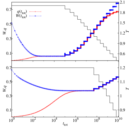
Figure 1: (Color online) Overview of our two annealing simulations for $H=0.2$. We show the evolution of $q(t_{\text{tot}})$ [the red (lower) curve] and $W(t_{\text{tot}})$ [the blue (uppe) curve] during the whole simulation. The continuous black line indicates the temperature throughout the simulation (see right-hand vertical axis for the scale). The top panel corresponds to the cold annealing and the bottom panel to the hot annealing (see Table 2). Notice how, in the former, the system is not able to reach equilibrium for the lowest temperatures (as signaled by different values of $W$ and $q$ at the end of each temperature step).

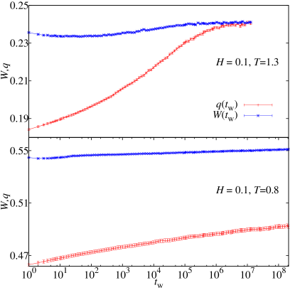
Figure 2: (Color online) Detail of our annealing simulation for $H=0.1$ at two different temperatures, $T=1.3$ and $T=0.8$. Notice how in the second case, despite the longer simulation time, the system does not reach equilibrium.

We show in Figure 1 an overview of our two sets of annealing runs for $H=0.2$. We represent both $W(t_{\text{tot}})$ and $q(t_{\text{tot}})$, which, for large $t_{\text{w}}$, should converge to the same value (in the paramagnetic phase). As we can see, in the cold annealing this condition is not satisfied for several of the lower temperatures, signaling that the system has fallen out of equilibrium. The hot annealing reaches the equilibrium regime for the whole temperature range.

A more detailed picture of these two regimes can be seen in Figure 2, which represents $W(t_{\text{w}})$ and $q(t_{\text{w}})$ for two temperatures and $H=0.1$. As we can see, for the higher temperature both observables converge to the same long-$t_{\text{w}}$ limit. For the lower temperature, however, the two quantities are far apart during the whole simulation and seem to have a different asymptote. This indicates that either the equilibration time is much larger than our simulation or we are in a spin-glass phase. Deciding between these two possibilities is the main goal of this paper.

III.2 Identification of intrinsic time scales

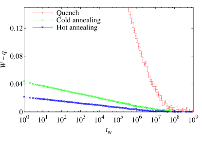
Figure 3: (Color online) Our three different simulations at $T=1.0$ for $H=0.2$. We show the difference $W-q$ as a function of the waiting time $t_{\text{w}}$, whose decay to zero determines the time scale of the simulations. Despite having very different initial conditions, the three simulation protocols need roughly the same time to reach equilibrium. We shall quantify this assertion in this Section III.2. Notice how, for the two annealing protocols, the behavior of $W-q$ is linear in $\log(t_{\text{w}})$ for a long time range.

Our strategy will rely on the study of the difference between $W(t_{\text{w}})$ and $q(t_{\text{w}})$ as a function of time, which should decay to zero in the high-temperature phase. Some inspiration comes from the classic paper by Ogielski Ogielski (1985), although we shall use other approaches as well.

We show in Figure 3 the behavior of $W(t_{\text{w}})-q(t_{\text{w}})$ for $T=1.0$ and $H=0.2$ using the three simulations protocols described in the previous section (direct quench and cold and hot annealing). Not surprisingly, the starting value of $W-q$ differs greatly from one protocol to the other. It is very large (well out of the graph’s scale) for the direct quench, which starts with a random configuration (representing a very high temperature) and it is smallest for the hot annealing, which has a small temperature step.

Nevertheless, all protocols seem to need roughly the same number of MCS to reach equilibrium, as evinced by the merging of the curves at $t_{\text{w}}\sim 10^{8}$. This observation gives us some hope of determining an intrinsic time scale $\tau$, depending only on the system’s temperature and not on its history.

In principle, the robust way to compute $\tau$ would be to perform a calculation analogous to Eq. (18), replacing $C$ by $W-q$ and $r$ by $t_{\text{w}}$. Unfortunately, in the interesting temperature range the maximum of the integrand $t_{\text{w}}^{k}[W-q](t_{\text{w}})$ is always in a region with a dismal signal-to-noise ratio (cf. Figure 1 in Belletti et al. (2009a)). Therefore, we have to resort to more phenomenological determinations.

A traditional way to identify this time scale, which was found adequate in the absence of a field Ogielski (1985), is fitting the difference $W(t_{\text{w}})-q(t_{\text{w}})$ to a stretched exponential decay:

$$W(t_{\text{w}})-q(t_{\text{w}})=\frac{\mathcal{A}}{t_{\text{w}}^{x}}\exp\left[-\left(\frac{t_{\text{w}}}{\tau^{\prime}}\right)^{\beta}\right]\,.$$ (34)

From this fit one gets a characteristic time $\tau^{\prime}$, which we can use as our time scale.

Computing a fit to Eq. (34) is difficult due to the extreme correlation of our data, which prevents us from inverting its full covariance matrix (necessary to define the $\chi^{2}$ goodness-of-fit indicator). Therefore, we consider only the diagonal part of the matrix in order to minimize $\chi^{2}$ and take correlations into account by repeating this procedure for each jackknife block in order to estimate the errors in the parameters. This is, of course, only an empirical procedure, but one that has been shown to work well under these circumstances (see, e.g., Belletti et al. (2009a), especially sections 2.4 and 3.2).

The results of these fits are gathered in Table 3. We do not report the value of the (diagonal) $\chi^{2}$/d.o.f. because it is, in all cases, $\chi^{2}/\text{d.o.f.}<1$ (as we have said this indicator does not give the full picture in the presence of strong data correlations). For each value of the magnetic field we have fitted up to the point where the system falls out of equilibrium (as indicated by a $\tau^{\prime}$ longer than the simulation time).

$H$	$T$	Annealing	Stretched exponential, Eq. (34)			Linear fit, Eq. (35)
			$\tau^{\prime}/10^{7}$	$\beta$		$\log(\tau^{\prime\prime})$	$\tau^{\prime\prime}/10^{9}$
0.3	1.0	Cold	0.015(7)	0.27(4)		14.69(12)	0.0024(3)
	0.9	Cold	0.09(4)	0.23(2)		17.20(15)	0.029(4)
	0.8	Cold	3.2(11)	0.21(2)		20.71(19)	0.99(19)
0.2	1.1	Cold	0.022(7)	0.30(4)		15.12(14)	0.0037(5)
		Hot	0.027(10)	0.37(6)		14.60(27)	0.0022(6)
	1.0	Cold	0.19(7)	0.26(3)		17.37(19)	0.035(7)
		Hot	0.14(6)	0.31(7)		16.9(3)	0.022(7)
	0.9	Cold	5.1(1.9)	0.23(3)		20.81(26)	1.1(3)
		Hot	3.1(2.2)	0.23(5)		20.2(6)	0.6(4)
0.1	1.4	Cold	0.0012(3)	0.40(4)		11.73(12)	0.000125(16)
	1.3	Cold	0.006(3)	0.32(5)		14.08(14)	0.00130(18)
	1.2	Cold	0.060(14)	0.34(3)		16.44(21)	0.014(3)

Table 3: Computation of characteristic times for several temperatures and simulation protocols using the stretched exponential (34) as well as a linear fit in $\log(t_{\text{w}})$ (35) ($\log$ being the natural logarithm). For each value of $H$ we report the last few temperatures before the system falls out of equilibrium. All the reported fits have (diagonal) $\chi^{2}/\text{d.o.f.}<1$.

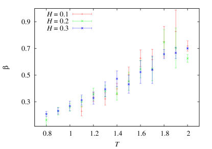
Figure 4: (Color online) Behavior of the stretching exponent $\beta$ (see Eq.(34)) as a function of $T$ for our three simulated magnetic fields.

A possible source of uncertainty in our determination of $\tau^{\prime}$ is the dependence of the fit on the value of $\beta$. Indeed, for each $T$ we are fitting simultaneously for $x$, $\mathcal{A}$, $\tau^{\prime}$ and $\beta$ in (34). However, a small variation in $\beta$ can have a large effect on $\tau^{\prime}$, which may lead us to think that the fit is unstable and unreliable. Fortunately (see Fig. 4), $\beta$ is actually a very smooth monotonic function of $T$, which leads us to believe that the fitting procedure is sound.

There is a final difficulty with this functional form: $\tau^{\prime}$ only has a straight interpretation as a correlation time (i.e., as an estimator for $\tau$) if $\beta\approx 1$. However, in the interesting temperature range, $0.2\lesssim\beta\lesssim 0.3$. This means that the actual value of $\tau^{\prime}$ cannot be interpreted directly as an estimator for $\tau$, but still we expect its divergence at the dynamical transition point to be intrinsic, as discussed in Section IV.

Notice, finally, that the values of $\tau^{\prime}$ and $\beta$ computed at the same temperature for the hot and cold annealing protocols for $H=0.2$ are compatible. This is a very good indication that these parameters have some intrinsic meaning.

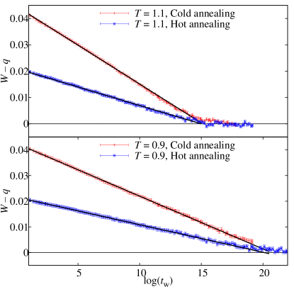
Figure 5: (Color online) Detail of our two annealing simulations for $H=0.2$ at two different temperatures, $T=1.1$ and $T=0.9$. We represent the difference $W-q$ as a function of $\log(t_{\text{w}})$ (we have used $\log$ as the natural logarithm throughout the paper). As pointed out in Figure. 3, in this representation $W-q$ is linear for a very long range. More interestingly, if we compute linear fits to (35) (continuous black lines), the intercepts with the horizontal axis are independent of the simulation protocol.

Another approach to the estimation of $\tau$, completely phenomenological, comes to mind from a visual inspection of Figure 3. Indeed, we can see that for both annealing protocols, the difference $W-q$ is linear in $\log(t_{\text{w}})$ for a very wide temperature range. This behavior is more clearly shown in Figure 5, which represents this quantity for two different temperatures.

Moreover, if we represent this linear behavior as

$$W(t_{\text{w}})-q(t_{\text{w}})\simeq\mathcal{B}\left[1-\frac{\log(t_{\text{w}})}{\log(\tau^{\prime\prime})}\right],$$ (35)

we can see from Figure 5 that the value of $\tau^{\prime\prime}$ does not depend on the annealing rate and is therefore dependent only on the temperature. Furthermore, since there is no stretching exponent, we can take $\tau^{\prime\prime}$ directly as an estimate of the actual intrinsic time scale of the system: $\tau^{\prime\prime}\approx\tau$.

Of course, Eq. (35) is only empirical and cannot be correct for very long times (it would predict an unphysical negative value of $W-q$ for $t_{\text{w}}>\tau^{\prime\prime}$), but its simplicity and robustness compensate for this problem. We give the values of $\tau^{\prime\prime}$ for several temperatures in Table 3 (in accordance with the previous discussion on the meaning of $\beta$, notice that $\tau^{\prime\prime}$ is more than an order of magnitude larger than $\tau^{\prime}$). In the following, we shall use both $\tau^{\prime}$ and $\tau^{\prime\prime}$ to study the possible critical behavior of the system.

IV The equilibrium regime

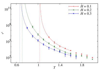
Figure 6: (Color online) Behavior of the characteristic time $\tau^{\prime}$ of the stretched exponential (34) as a function of the temperature for the three magnetic fields simulated. We also plot our fits to a power-law divergence of $\tau^{\prime}$ for a finite temperature, Eq. (36).

In this section we consider the temperature dependence of the characteristic time scales $\tau$ identified in Sect. III.2. Following Ogielski Ogielski (1985) as well as experimental studies (e.g., Jonsson et al. (1999)), we shall fit our equilibrium data to power-law divergence:

$$\tau=\frac{\tau_{0}}{\bigl{[}T-T_{\text{c}}(H)\bigr{]}^{\nu z}}\,,$$ (36)

where $\tau_{0}$ is a microscopical time. We use the traditional notation, where $T_{\text{c}}(H)$ is a critical temperature, $\nu$, is the correlation length critical exponent and $z$ is the dynamical critical exponent. However, as we shall see in Section VI, this divergence may or may not correspond to an actual phase transition at $T_{\text{c}}(H)$.

In Figure 6 we show the relaxation time $\tau^{\prime}$ computed with the stretched exponential (34) in Table 3 as a function of temperature for the three simulated magnetic fields. We also show fits to the power-law divergence at finite $T_{\mathrm{c}}^{\mathrm{high}}(H)$ (the superscript “high” refers to the fact that we are using high-temperature data, cf. Section V). We have obtained the following values:

• $H=0.1$: $T_{\text{c}}^{\text{high}}=1.03(7)$ and $z\nu=4.8(1.1)$. Using only $1.2\leq T\leq 1.7$ [$\chi^{2}/\mathrm{d.o.f.}=1.47/3$].

• $H=0.2$: $T_{\text{c}}^{\text{high}}=0.71(6)$ and $z\nu=7.5(1.1)$. Using only $0.9\leq T\leq 1.6$ [$\chi^{2}/\mathrm{d.o.f.}=3.36/5$].

• $H=0.3$: $T_{\text{c}}^{\text{high}}=0.66(5)$ and $z\nu=6.2(9)$. Using only $0.8\leq T\leq 1.5$ [$\chi^{2}/\mathrm{d.o.f.}=1.74/5$].

In all the fits we go down to the lowest temperature where we can measure $\tau^{\prime}$ reliably. The choice of the fitting range is not critical, several temperatures can be added or eliminated without altering the results significantly (especially in the high-temperature end). For $H=0.2$, we use the $\tau^{\prime}$ for the cold annealing, since they have smaller error bars than those for the hot annealing. We have checked that the $\tau^{\prime}$ at $T=0.85$ extrapolated with the above fits for the cold annealing is compatible with the corresponding correlation time measured in the hot annealing.

However, as we discussed in the previous section, $\tau^{\prime}$ does not have a straightforward interpretation as a relaxation time, since $\beta\neq 1$. Therefore, the above values of $T_{\mathrm{c}}^{\mathrm{high}}$ might be an artifact of our way of estimating $\tau$. In order to dispel this possibility, we have recomputed the fits to (36), this time using the relaxation time $\tau^{\prime\prime}$ computed with the linear fit in $\log t_{\text{w}}$ (35). Now the fit parameters are:

• $H=0.1$: $T_{\text{c}}^{\text{high}}=0.98(3)$ and $z\nu=7.2(5)$. Using only $1.2\leq T\leq 1.7$ [$\chi^{2}/\mathrm{d.o.f.}=4.21/3$].

• $H=0.2$: $T_{\text{c}}^{\text{high}}=0.670(21)$ and $z\nu=9.2(4)$. Using only $0.9\leq T\leq 1.6$ [$\chi^{2}/\mathrm{d.o.f.}=1.79/5$].

• $H=0.3$: $T_{\text{c}}^{\text{high}}=0.614(17)$ and $z\nu=8.4(4)$. Using only $0.8\leq T\leq 1.3$ [$\chi^{2}/\mathrm{d.o.f.}=2.61/3$].

We can see that we obtain good values of the goodness-of-fit estimator $\chi^{2}$ for all fits. The values of $T_{\text{c}}(H)$ are consistent for both sets of fits, while the values of $z\nu$ are a little higher for the fit with $\tau^{\prime\prime}$ ($2.0$ standard deviations for $H=0.3$, $1.5$ standard deviations for $H=0.2$ and $2.2$ standard deviations for $H=0.1$).

The consistency between these two sets of fits makes us confident that the observed divergence in the relaxation times is an intrinsic phenomenon and not an artifact of our simulation protocol or of our ansatz for the behavior of $W-q$.

IV.1 The relaxation time in the supercooled liquids approach

As discussed in Section II.4, the MCT predicts a divergence of the autocorrelation time at a temperature $T_{\text{d}}$, as in Eq. (29). In principle, Eq. (29) is exactly the same as Eq. (36), which we have just used to characterize the growth of the relaxation times. The crucial difference is that we have used our lowest thermalized temperatures and have assumed that the growth of $\tau$ was related to an actual critical divergence (as evinced by our notation of $z\nu$ for the exponent). On the other hand, in the supercooled liquids literature, Eq. (29) is used in a higher temperature range corresponding to $10^{2}<\tau<10^{4}$ (notice, for instance, that our values of $z\nu$ are very high compared to the values of $\gamma$ that can be found in the MCT literature). For lower temperatures, the behavior of $\tau$ deviates from (29), because of the emergence of activated processes.

Therefore, if we wanted to follow a supercooled liquids approach, we should first fit $\tau^{\prime}$ to (29) in the high temperature range and then move on to an exponential growth:

$$\tau^{\prime} =\frac{\mathcal{C}}{(T-T_{\text{d}})^{\gamma}}, \tau^{\prime}\lesssim 10^{4},$$ (37)

$$\tau^{\prime} =\exp\bigl{[}\mathcal{D}/(T-T_{\text{c}})^{\gamma^{\prime}}\bigr{]}, \tau^{\prime}\gtrsim 10^{4}.$$ (38)

Unfortunately, our simulations are not suited to the determination of small $\tau$, so the fit to (37) will probably be plagued by strong systematic effects.

We consider only $H=0.2$ (for $H=0.1$ we have too narrow a temperature range and for $H=0.3$ our fits for $\tau^{\prime}$ are rather unstable for $T>1.7$). We have fitted $\tau^{\prime}$ to (37) in the range $1.3\leq T\leq 1.9$ (which corresponds to $10^{2}<\tau^{\prime}<10^{4}$). The result is $T_{\text{d}}=1.22(6)$ with $\gamma=2.1(7)$ ($\chi^{2}/\text{d.o.f.}=0.94/4$). The next step would be to take $\tau^{\prime}$ in the range $T\leq 1.3$ (which we have previously fitted successfully to a critical divergence with $z\nu\approx 8$) and attempt a fit to (38) instead. Unfortunately, fitting for $T_{\text{c}}$ and $\gamma^{\prime}$ simultaneously is simply not possible with our data (the resulting error in $T_{\text{c}}$ is greater than $100\%$). In short, we can only say that a temperature dependence of $\tau$ according to (37) and (38) cannot be excluded, but we cannot make this statement more quantitative. Nevertheless, we shall return to the possibility of activated dynamics in Sections V.2 and VI.

V Non-equilibrium regime

As already explained in Section III.2, our annealing rate eventually becomes too fast, compared to the growth of $\tau(T)$ upon cooling. At that point, the simulation falls out of equilibrium. We enter here the reign of extrapolation, which is always rather risky.

We shall extrapolate our data to long times following two very different strategies. In Section V.1 we extrapolate using power laws. The outcome will be consistent with the RSB theory. On the other hand, in Section V.2 we use the linear-log extrapolation (see Sect. III.2), which assumes from the outset that no phase transition occurs.

V.1 Power-law extrapolations to long times

So far, we have been working in the high-temperature phase, where $W-q$ goes to zero for long times. We saw that, as we lower the temperature, the associated relaxation time grows very quickly and eventually becomes much larger than our simulations. This rapid growth was actually consistent with a power-law divergence of $\tau$ at finite $T$.

In this section we shall take a complementary approach. We now work in the low-temperature regime, where $\tau$ is either infinite or, at the very least, much larger than our simulation times. In this regime, rather than assuming that $W-q$ goes to zero for long times, we can try to extrapolate for a (possibly) non-zero asymptote.

Following the literature Parisi et al. (1998); Marinari et al. (1998a), we shall first attempt a study in the total annealing time $t_{\text{tot}}$, considering different annealing rates (Section V.1.1). Then we shall repeat the analysis using only $t_{\text{w}}$ (as in the rest of the paper) in Section V.1.2.

V.1.1 Study in $t_{\text{tot}}$ for different annealing rates

In the limit of a very slow annealing, the simplest ansatz for the low-temperature behavior of $W-q$ is a power-law decay (cf. Ogielski (1985)):

$$W(t_{\text{tot}})-q(t_{\text{tot}})=a(T,H)+\frac{b}{t_{\text{tot}}^{x}}\,.$$ (39)

Eventually $b$ and $x$ could also depend on the temperature Ogielski (1985) and on the external magnetic field. Notice that, in contrast with the rest of the paper, here we are considering the total time $t_{\text{tot}}$ since the simulation started Parisi et al. (1998); Marinari et al. (1998a), not just the time $t_{\text{w}}$ since the last temperature change.

Should the system experience a spin-glass transition, we would expect $a(T,H)>0$ for very low $T$ [recall Eq. (28)]. This asymptote would decrease as we increase the temperature until eventually, at some temperature $T_{\text{c}}^{\mathrm{low}}(H)$, $a\bigl{(}T_{\text{c}}^{\mathrm{low}}(H),H\bigr{)}=0$. This description is consistent with a qualitative look at $W-q$ (recall, for instance, Figure 2).

If the RSB picture is correct, we would expect $T_{\text{c}}^{\mathrm{low}}(H)$ to coincide with the divergence of $\tau$ and signal a thermodynamic phase transition, that is, $T_{\text{c}}^{\mathrm{low}}(H)=T_{\text{c}}^{\mathrm{high}}(H)=T_{\text{c}}$.

Equation (39), with $a>0$, should hold only deep in the spin-glass phase. If we approach the transition from below (in temperature) we would start to see the critical effects of the (thermodynamical) critical point, and the exponent $x$ would begin to be controlled by this critical point and not by the “critical” spin-glass phase (Goldstone phase). So, in the critical region we should expect:

$$W(t_{\text{tot}})-q(t_{\text{tot}})=\frac{f}{t_{\text{tot}}^{x_{c}}}\,,$$ (40)

where in general $x_{c}$ (driven by the critical point) should be different from $x$ (driven by the spin-glass phase).

From the previous discussion, and assuming the onset of a phase transition, it is clear that the $x$ exponent should take a constant value at lower temperatures (here we are assuming that the phase transition is universal in the magnetic field), then change as we reach the critical region.

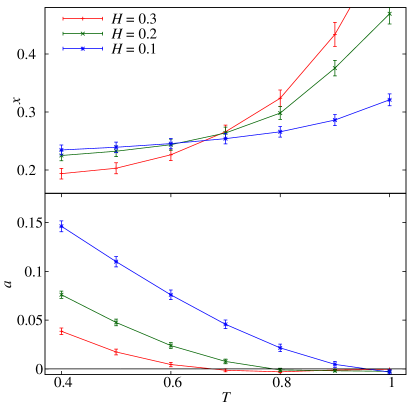
Figure 7: (Color online) Top: Exponent $x$ of the extrapolation of the difference between $W(t_{\text{tot}})$ and $q(t_{\text{tot}})$, Eq. (39), as a function of temperature, for our three external magnetic fields. Value computed from three-parameter fits. Bottom: As above, for the asymptote $a$.

Now, in order to study the decay of $W-q$ we obviously need to follow the time evolution along several orders of magnitude. However, as described in Section III.1, for a fixed temperature $T_{k}=T_{\text{init}}-k\Delta T$ the total time elapsed in our annealing simulations varies in the range $t_{k}(t_{\text{base}})\leq t_{\text{tot}}\leq t_{k+1}(t_{\text{base}})\sim 2t_{k}(t_{\text{base}})$, which is too narrow in a logarithmic scale. Therefore, instead of analyzing the data for all the $t_{\text{tot}}$ in a given annealing simulation, we shall combine all our cold annealing simulations for different values of $t_{\text{base}}$. That is, for each temperature $T_{k}$ we take the value of $W-q$ at $t_{k+1}(t_{\text{base}})$, for $t_{\text{base}}=10^{i}$, $i=0,\ldots,5$. Thus, we get for each temperature $T_{k}$ a series of six values of $[W-q](t_{\text{tot}})$ in the range $t_{k+1}(t_{\text{base}}\!=\!1)\leq t_{\text{tot}}\leq t_{k+1}(t_{\text{base}}\!=\!10^{5})$, which we fit to (39) [recall that $t_{k+1}(t_{\text{base}})=(2^{k+1}-1)t_{\text{base}}$].

The resulting values of $a(T)$ and $x(T)$ are plotted in Figure 7. As we can see, the qualitative picture is very much what we painted above. In particular, we obtain a positive value of the asymptote $a$ for low temperatures, which goes to zero at a temperature $T_{\text{c}}^{\text{low}}$ not very different from $T_{\text{c}}^{\text{high}}$ —we can estimate $T_{\text{c}}^{\text{low}}(H=0.3)\approx 0.65(5),T_{\text{c}}^{\text{low}}(H=0.2)\approx 0.80(5),T_{\text{c}}^{\text{low}}(H=0.1)\approx 0.96(5)$. In addition, the value of the exponent $x$ is roughly constant (and independent of $H$) at low temperatures, while it grows noticeably as we approach $T_{\text{c}}^{\text{low}}$.

However, we must caution the reader that the fits we have just discussed are rather delicate. In particular, even after discarding the two smallest $t_{\text{tot}}$ (so we are left with a three-parameter fit to four points), we find that values of the $\chi^{2}$ goodness-of-fit estimator are sometimes very high. In particular, the fits for $H=0.1,0.3$ are good in the interesting temperature range (always $\chi^{2}/\text{d.o.f.}\leq 1.5/1$), but those for $H=0.2$ have $\chi^{2}/\text{d.o.f.}$ that can be in excess of $8/1$, clearly unacceptable. More worryingly, if we shift the fitting window we find that the fitted values for $x$ and $a$ decrease noticeably with increasing $t_{\text{tot}}$ (the change in $x$ can be as high as $50\%$ just by shifting the fitting window so that we discard the longest time but include an extra point in the lower end of the range). Still, for $H=0.1,0.3$ only the fitting window for the longest $t_{\text{tot}}$ gives reasonable fits (for $H=0.2$ the situation is murkier, since the fits are poor in any case). It will be interesting to compare these values with the ones we shall obtain in the next section (Section V.1.2), with a study in $t_{\text{w}}$.

Of course, from the above arguments one could think that, for long enough $t_{\text{ttot}}$, the exponent could decrease so much that the asymptote $a$ would become zero. In order to check against that possibility, and to obtain a sort of lower bound for $a$, we have also attempted fits to the following function

$$W(t_{\text{tot}})-q(t_{\text{tot}})=a^{\prime}+\frac{b^{\prime}}{\log(t_{\text{tot}})^{x^{\prime}}}.$$ (41)

Using this fitting function we get good fits with values of $x^{\prime}\approx 3$ and positive $a^{\prime}$ for $T<T_{\text{c}}^{\text{high}}$, so the qualitative picture is the same. The determination of $T_{\text{c}}^{\text{low}}$ is a little lower, but still compatible with our $T_{\text{c}}^{\text{high}}$.

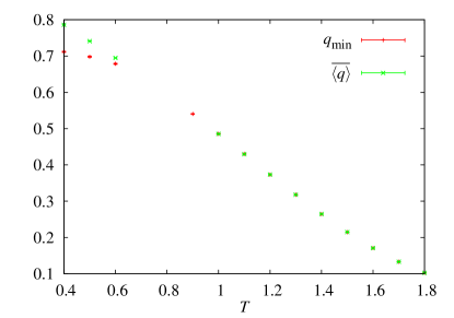
Figure 8: (Color online) Extrapolations to infinite time of $W(t_{\text{tot}})\to\overline{\langle q\rangle}$ and $q(t_{\text{tot}})\to q_{\text{min}}$ for $H=0.2$, according to (42). We use the same exponent $x$ computed in Figure 7.

The next step in this study is the investigation of the scaling in $W$ and $q$ separately. To this end, we are going to consider fits of the form

$$\begin{split}W(t_{\text{tot}})&=\overline{\langle q\rangle}+\frac{b^{\prime\prime}}{t_{\text{tot}}^{x}},\\ q(t_{\text{tot}})&=q_{\text{min}}+\frac{b^{\prime\prime\prime}}{t_{\text{tot}}^{x}},\end{split}$$ (42)

where for both observables we take the same value of $x$ that we computed in Figure 7. The resulting plots of $\overline{\langle q\rangle}(T)$ and $q_{\text{min}}(T)$ can be seen in Figure 8 for $H=0.2$. Except for $H=0.2$, we obtain excellent fits both for $q$ and for $W$ ($\chi^{2}/\text{d.o.f.}<1$). For high temperatures ($T\geq 0.9$ for $H=0.2$) we do not need to extrapolate, since we reach equilibrium in our annealing simulations. There is a small gap with no extrapolations, corresponding to temperatures above $T_{\text{c}}$, where (39) does not work but we cannot reach equilibrium. The qualitative picture is what one would expect in the RSB scenario.

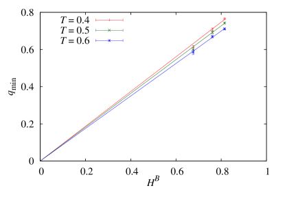
Figure 9: (Color online) Scaling of the minimum overlap with the magnetic field. A simple power-law behavior, $q_{\text{min}}\sim H^{B}$, works well for all our subcritical temperatures, even though we are far from the small-$q_{\text{min}}$ limit.

Finally, we can consider the scaling of $q_{\text{min}}$ with the magnetic field at fixed temperature. As the magnetic field goes to zero, so must $q_{\text{min}}$ and we could expect a behavior of the kind $q_{\text{min}}(H)\sim H^{B}$. Indeed, a rough dimensional analysis Marinari et al. (1998a) tells us that $B=\theta(0)/[D-\theta(0)/2]$, where the replicon exponent in $D=3$ is $\theta(0)=0.39(5)$ Alvarez Baños et al. (2010b). Therefore, we expect a value of $B=0.14(2)$. We have computed fits to

$$q(H)=\mathcal{C}H^{B}$$ (43)

for $T=0.4,0.5$ and $0.6$ (the only temperatures that are below $T_{\text{c}}$ for our three magnetic fields). The results are $B(T=0.4)=0.20(2)$, $B(T=0.5)=0.19(2)$, $B(T=0.6)=0.17(2)$, very close to our expected $B=0.14(2)$ (notice that we are considering rather high magnetic fields, as evinced by the high values of $q_{\text{min}}$ that we are seeing). In all cases we obtain excellent values of the $\chi^{2}$ estimator. We have plotted $q_{\text{min}}^{B}$ in Figure 9, using for all fields an intermediate value of $B=0.18$.

V.1.2 Study in $t_{\text{w}}$

As discussed above, the total time $t_{\text{tot}}$ since the simulation started is the more physical variable to conduct the low-temperature study. However, we have seen in Sections III.1 and IV that we can also study the relaxation of the system in $t_{\text{w}}$ in a consistent way. Therefore, it is interesting to repeat the study of Section V.1.1 taking only our slowest cold annealing (with $t_{\text{base}}=10^{5}$) and studying for each temperature the relaxation in $t_{\text{w}}$.

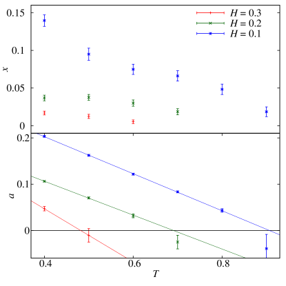
Figure 10: (Color online) Top: Exponent $x$ of the extrapolation of the difference between $W(t_{\text{w}})$ and $q(t_{\text{w}})$, Eq. (44), as a function of temperature, for our three external magnetic fields. Values computed in a three-parameter fit. Bottom: As above, for the asymptote $a$. Lines are linear fits to the points where $a(T,H)>0$ (for $H=0.3$ we included as well $T=0.5$ in the fit).

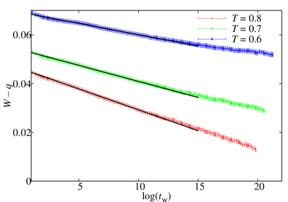
Figure 11: (Color online) $W-q$ as a function of $\log(t_{\text{w}})$ for several low temperatures and $H=0.2$. Even in this temperature range we can identify a wide linear regime.

To this end we consider an equation analogous to (39):

$$W(t_{\text{w}})-q(t_{\text{w}})=a+\frac{b}{t_{\text{w}}^{x}}.$$ (44)

We have computed fits to (44) for all our lower temperatures, finding that the power-law decay describes the behavior of $W-q$ with great precision. Indeed we find for the standard figure of merit $\chi^{2}/\mathrm{d.o.f.}<0.5$ (such a small value is due to the strong data correlation and to the fact that we are computing $\chi^{2}$ only with the diagonal part of the covariance matrix). We show in Figure 10 the fit parameters of $x$ and $a$ as a function of temperature (upper and lower panels respectively). Clearly, this study leads to much lower values of $x$ than the analysis in $t_{\text{tot}}$ (but recall that in the previous section the value of $x$ decreased if we shifted the fitting window to longer times, a problem we do not have here). Indeed, the values of $a$ are more similar to those computed with (41). Finally, let us recall that relaxation exponents of $\mathcal{O}(10^{-2})$ have already been seen in the $H=0$ case Belletti et al. (2009a).

In any case, the qualitative picture is just the same as in our previous section, although the values of $x$ are much lower. This is because, since we are using the run with the longest $t_{\text{base}}$, the effective time at $t_{w}=0$ is large (in other words, $W-q$ is already very low at $t_{w}=0$, since it has already evolved for a considerable time at higher temperatures).

Again, we can use the temperature at which $a$ becomes zero as our estimate of $T_{\text{c}}^{\mathrm{low}}(H)$. We note in Figure 10–bottom that the statistical errors for $a$ are small only when it is positive. Hence we have located the zeros by performing first a linear fit to these points, and then finding the root of the linear function. In order to take care of the extreme data correlation, we use a jackknife procedure: fit with the diagonal part of the covariance matrix, but then perform separate fits for each jack-knife block Belletti et al. (2009a). We obtain $T_{\text{c}}^{\mathrm{low}}(H=0.3)=0.48(2)$, $T_{\text{c}}^{\mathrm{low}}(H=0.2)=0.69(1)$, $T_{\text{c}}^{\mathrm{low}}(H=0.1)=0.906(6)$.

Similarly, we can extrapolate $q(t_{\text{w}})$ and $W(t_{\text{w}})$ to infinite time separately. Again, we obtain $\chi^{2}/\text{d.o.f.}<1$ in all cases for $t_{\text{w}}\gtrsim 1000$. We do not reproduce the resulting picture, since it is essentially the same as Figure 8 (with a slightly higher value for $q_{\text{min}}$ at low $T$).

In short, we can say that assuming a power-law decay of $W-q$ at low temperatures leads to a picture consistent with a RSB spin-glass transition at $T_{\text{c}}^{\mathrm{low}}(H)\approx T_{\text{c}}^{\mathrm{high}}(H)$.

V.2 Assuming no phase transition: linear-log extrapolations to large times

In the previous section we assumed that the decay of $W-q$ followed a power law at low temperatures and tried to determine the point where the asymptote became positive. In this section we take the opposite approach and will assume that there is no phase transition, that is, that $W-q$ goes to zero for all $T>0$.

In order to do that, we are going to recall our phenomenological expression (35), which, at high temperature, described a wide time range where $W-q$ was linear in $\log(t_{\text{w}})$. In Section III.2 we used this functional form to estimate a characteristic time scale $\tau^{\prime\prime}$. Naturally, the real curve $W-q$ must deviate from (35), otherwise it would become negative for $t>\tau^{\prime\prime}$, but at high temperature we found that the curvature was noticeable only at the very end of the simulation, where $W-q$ was already very small (even compatible with zero).

$H$	$T$	$\log(\tau^{\prime\prime})$	$T\log(\tau^{\prime\prime})$
0.3	0.7	27.9(4)	19.55(26)
	0.6	43.0(7)	25.8(4)
	0.5	80.2(1.3)	40.1(6)
	0.4	179(4)	71.5(1.5)
0.2	0.8	28.4(6)	22.7(4)
	0.7	42.6(9)	29.8(6)
	0.6	78.8(1.8)	47.3(1.1)
	0.5	178(6)	89.1(2.8)
	0.4	409(13)	163(6)
0.1	1.0	26.7(6)	26.7(6)
	0.9	39.9(9)	35.9(8)
	0.8	67.6(1.6)	54.1(1.3)
	0.7	115(3)	80.6(2.3)
	0.6	226(6)	135(4)
	0.5	450(14)	225(8)
	0.4	—	—

Table 4: Computation of a lower bound for the relaxation time at low temperature using the linear fit in $\log(t_{\text{w}})$ of Eq. (35). For each $H$ we include the values of $\log(\tau^{\prime\prime})$ for temperatures in the non-equilibrium regime (i.e., lower than those included in Table 3). For $H=0.1$ and $T=0.4$ the curve $W-q$ is flat within errors and we cannot determine any $\log(\tau^{\prime\prime})$. Data from the cold annealings.

In this section, we are going to use (35) in order to obtain a lower bound for the relaxation time of the system. Indeed, if we look at Figure 11, we can see that even for very low $T$ the difference $W-q$ behaves linearly in $\log(t_{\text{w}})$ for a long time scale, before slowing down its decay. Therefore, in the very reasonable assumption that there is no convexity change, we can use the parameter $\log(\tau^{\prime\prime})$ of the linear fit in order to obtain a lower bound for the actual relaxation time $\tau$ of the system.

With this procedure, we obtain a finite lower bound for $\tau$ even for very low temperatures (see Table 4). The resulting values of $\log(\tau^{\prime\prime})$ are enormous (as an amusing comparison, the age $\mathcal{T}$ of the universe measured in MCS is $\log(\mathcal{T})\sim 68$, much smaller than some of the measured $\tau^{\prime\prime}$). Therefore, even a rather loose lower bound gives us a wildly growing time scale.

In order to make this statement more quantitative, let us recall that, in the droplet picture, $\xi(H,T)$ is finite even at $T=0$ for $H>0$. Therefore, for low temperatures we would expect

$$\log\tau=\xi(0,H)^{\Psi}/T,$$ (45)

or, in other words, we would expect $T\log(\tau)$ to be constant. However, see Table 4, we find that even our lower bound $\log(\tau^{\prime\prime})$ grows much faster than predicted by the droplet theory.

We can take this one step further. In Figure 12 we have plotted $T\log(\tau^{\prime\prime})$ against $T$ in a log-log scale. As we can see, the data for low temperature are well described by a Vogel-Fulcher-Tammann divergence at $T=0$:

$$T\log(\tau^{\prime\prime})=\frac{A}{T^{c}}\ .$$ (46)

A fit to (46) for our three magnetic fields gives:

• $H=0.1$, $c(H=0.1)=3.05(10)$, fitting in $T\leq 0.7$, with $\chi^{2}/\text{d.o.f.}=2.1/1$.

• $H=0.2$, $c(H=0.2)=3.09(6)$, fitting in $T\leq 0.7$, with $\chi^{2}/\text{d.o.f.}=4.1/2$.

• $H=0.3$, $c(H=0.2)=2.50(5)$, fitting in $T\leq 0.6$, with $\chi^{2}/\text{d.o.f.}=0.80/1$.

We can see that $H=0.1$ and $H=0.2$ even have the same exponent, while $\log(\tau^{\prime\prime})$ grows a little more slowly for $H=0.3$ (this is probably because we have not reached low enough temperatures at $H=0.3$).

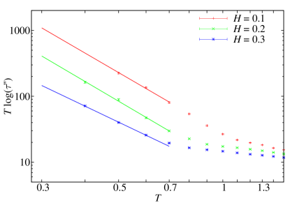
Figure 12: (Color online) Plot of a lower bound for $T\log(\tau)$, computed using (35), against $T$ for our three magnetic fields. At very low temperatures this quantity is compatible with a Vogel-Fulcher-Tammann divergence at $T=0$, Eq. (47). Notice the change of regime at around $T_{\text{c}}^{\mathrm{high}}(H)$ (recall Figure 6).

Actually, the data in Figure 12 admit fits of a more general form

$$T\log(\tau^{\prime\prime})=\frac{A}{(T-T_{*})^{c}}\ ,$$ (47)

where $|T_{*}|$ is very small but $T_{*}$ could even be negative. Unfortunately, we do not have enough degrees of freedom to fit simultaneously for $c$ and $T_{*}$. We shall discuss the possible implications of this $T_{*}$ in the following section.

Notice, finally, that in Figure 12 we can appreciate a sharp change of regime precisely around the temperature where we identified a power-law divergence of $\tau$, fitting from the high-temperature phase.

In the following section we shall introduce a more direct study of $\xi$ and try to combine the results of Sections IV and V in a consistent physical picture.

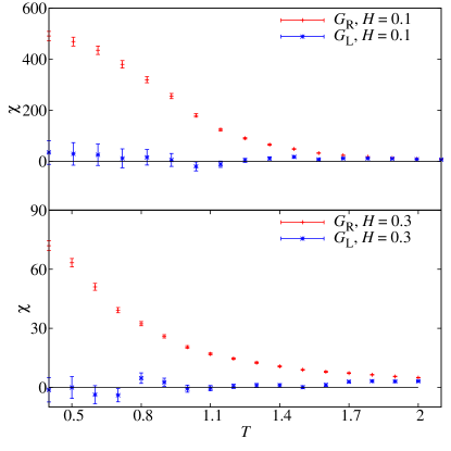
Figure 13: (Color online) Replicon and longitudinal susceptibilities in our cold annealings for $H=0.1,0.3$ (we plot the last $t_{\text{w}}$ for each $T$). The plot contains both equilibrium and non-equilibrium data.

VI Dynamics and the correlation length

Up to now, we have focused on the determination of characteristic times and their temperature dependence. However, a proper discussion of any phase transition requires as well the consideration of spatial correlation and the correlation length (this is, in fact, a longstanding obstacle in the investigation of structural glasses Weeks et al. (2000); Berthier et al. (2005); Montanari and Semerjian (2006)). In the framework of spin glasses we are advantaged, because the structure of correlators has been investigated in detail (see Section II.2 and references therein). In particular, there are two types of correlation functions to deal with, the replicon and the longitudinal/anomalous correlator. We shall first decide which of the two correlators is worth studying and check that equilibrium results can indeed be obtained in some temperature range (Section VI.1). At that point, we shall revisit the the dynamics on the view of the correlation length (Section VI.2).

VI.1 Which correlation function?

We compare in Figure 13 the replicon and longitudinal/anomalous susceptibilities [recall Eq. (16)], for $H=0.1,0.2$ and $0.3$. The susceptibilities are shown as a function of temperature, as computed for the latest time on each temperature step along the cold annealing. This means that Figure 13 contains both equilibrium and non-equilibrium data (depending on whether the constant-temperature step is much larger than $\tau$, or not). In either case, it is rather obvious that significant correlations appear only on the replicon correlator (in agreement with equilibrium, mean-field computations de Almeida and Thouless (1978)). Therefore, we focus on the replicon correlator from now on. The anomalous sector is studied in more detail in Appendix B, Section B.3.

We note as well that the failure of the longitudinal/anomalous correlator to display the correlations relevant to the problem might be related to analogous failures in experimental investigations of structural glasses Debenedetti (1997); Debenedetti and Stillinger (2001).

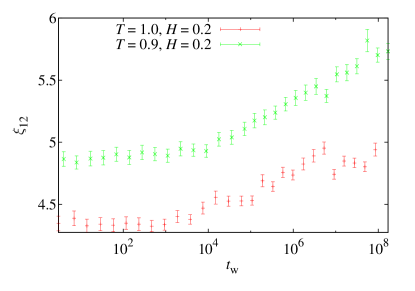
Figure 14: (Color online) Equilibration of the correlation length: for $H=0.2$, we show the $\xi_{12}$ correlation length as computed from the replicon correlator $G_{\text{R}}$ as a function of $t_{\text{w}}$. We display data for two constant-temperature steps in the cold annealing (recall that $t_{\text{w}}$ is the time elapsed since the last temperature drop). The constant temperature time step is longer than $\tau$ only for $T=1.0$.

Specifically, we consider the $\xi_{12}$ correlation length as computed from the replicon correlator $G_{\text{R}}$ using Eq. (18). Its time evolution for two constant-temperature steps in the cold annealing run is displayed in Figure 14. For both temperatures we identify three regimes. For short $t_{\text{w}}$ the correlation length basically remains constant (the fact that $\xi_{12}$ does not decrease at $t_{\text{w}}\sim 1$ is interesting in itself: it tells us that temperature chaos effects are weak). Then, the time evolution starts to be noticeable and $\xi$ starts to increase. Finally, when $t_{\text{w}}\gg\tau$, the correlation length becomes time-independent, which is consistent with our physical interpretation in Section IV that thermal equilibrium has been reached. We note as well that the equilibrium regime is barely reachable for $T=0.9$ —remember that $\tau^{\prime\prime}(T=0.9)=1.1(3)\times 10^{9}$, while $\tau^{\prime\prime}(T=1.0)=1.8(7)\times 10^{7}$. In the next paragraph, we shall discuss $\xi_{12}$ as a function of temperature, but only for those temperatures where thermal equilibrium can be reached.

VI.2 Dynamics from the point of view of the correlation length

An important question is: is the dynamics activated [ $\tau\sim\mathrm{e}^{\xi^{\varPsi}/T}$, Eq. (24)], or critical [$\tau\sim\xi^{z}$, Eq. (26)]?

As explained in Section II.3, the droplet theory supports activated dynamics. On the other hand, the RSB theory is somewhat ambiguous on this point [at mean-field level the dynamics is critical, this is the rationale for using $z\nu$ as the critical exponent in Eq. (36)]. Furthermore, current theories for supercooled liquid relaxations predict both types of behaviors (Section II.4). These theories expect critical dynamics at high temperatures, with an effective exponent $z_{\mathrm{MCT}}=4\gamma$ [recall Eqs. (29,30)]. However, at lower temperatures the dynamics should crossover to an activated behavior.

At this point, we have in our hands equilibrium determinations for both $\tau(T,H)$ and $\xi_{12}(T,H)$. Therefore, we can try to assess Eqs. (24,26) directly. This is attempted in Figure 15, where we used $\tau^{\prime\prime}$ from fits to Eq. (35). Although this choice is arbitrary to some extent, we recall that the critical divergence studied in Section IV turned out to be independent on the choice of $\tau$.

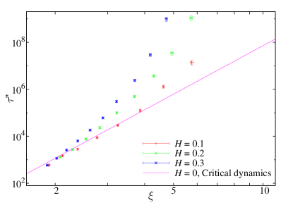
Figure 15: (Color online) Logarithmic plot of $\tau^{\prime\prime}$, computed in Section III, versus the correlation length ($\xi_{12}$) for the three magnetic fields simulated. Data are in equilibrium. For comparison, we also show the critical dynamics for $H=0$, $\tau\sim\xi^{z}$, with $z=6.86$ Belletti et al. (2009a).

We note two different regimes in Figure 15. For high-temperatures, data follow a critical dynamics. However, at lower temperatures (i.e., larger $\xi$) $\tau$ starts to grow much faster with $\xi$. In fact, the effective exponent $z^{\text{eff}}=\mathrm{d\,log\,}\xi/\mathrm{d\,log\,\tau}$ becomes as large as $z^{\text{eff}}\approx 14$, which clearly suggest that the dynamics is becoming activated. Overall, this crossover exemplifies the behavior expected for a supercooled liquid. In fact, critical dynamics is found in the range $10^{2}<\tau<10^{4}$, which is also the range where MCT applies for simple supercooled liquids Kob and Andersen (1994). However, an alternative interpretation is possible. First, one may note that we identified in Section IV.1 an exponent $\gamma\approx 2$. Considering the large uncertainty in this determination, this is consistent, via Eqs. (29) and (30), with the $z_{\text{eff}}\approx 7$ that we find in Figure 15. However, the slope in the figure is also very close to $z_{H=0}=6.86$, the value for the critical dynamics in the absence of a magnetic field Belletti et al. (2009a). Hence, the crossover can be also due to the proximity of the Renormalization-Group fixed point at $(T_{\mathrm{c}},H=0)$. In fact, the larger $H$ is the smaller the $\xi$ needed to find activated dynamics (see Figure 15).

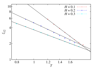
Figure 16: (Color online) Logarithmic plot of the equilibrium correlation length $\xi_{12}$ versus the temperature for the three magnetic fields simulated. Lines are fits to $\xi_{12}(T)=a_{H}/T^{b_{H}}$, see Eq. (48). When assessing the high-temperature data for $H=0.1$, recall that the critical temperature without a field is $T_{\mathrm{c}}^{H=0}=1.1019(29)$ Baity-Jesi et al. (2013).

Let us consider the temperature evolution of $\xi_{12}$ in equilibrium, see Figure 16. We do not find good fits to critical divergences, $\xi_{12}\propto 1/|T-T_{\mathrm{c}}(H)|^{\nu}$, with $T_{\mathrm{c}}(H)$ compatible with the characteristic temperatures identified in Section IV. For instance, a fit for $H=0.2$ gives a reasonable $\chi^{2}$ value only for $T_{\text{c}}\lesssim 0.5$, while at $H=0.1$ we get $T_{\text{c}}\lesssim 0.8$ (these bounds are very crude, since we have almost no degrees of freedom for the fits). In particular, assuming that $T_{\text{c}}=0$ we still get good fits:

$$\xi_{12}(T) = \frac{a_{H}}{T^{b_{H}}}\,,$$ (48)

$$b_{H=0.1} = 2.52(4)\quad(1.2\leq T\leq 1.5,\chi^{2}/\text{dof}=1.9/2)\,.$$ (49)

$$b_{H=0.2} = 1.55(4)\quad(0.9\leq T\leq 1.2,\chi^{2}/\text{dof}=3.6/2)\,.$$ (50)

$$b_{H=0.3} = 1.10(5)\quad(0.8\leq T\leq 1.0,\chi^{2}/\text{dof}=0.25/1)\,.$$ (51)

Hence, at least within the temperature range that can be equilibrated, our data are compatible with a divergence of $\xi$ only for very low (perhaps even vanishing) $T_{\mathrm{c}}(H)$. Notice, however, that we are always working with $\xi<6$, so this kind of fit is rather dangerous.

At this point, is is only natural to ask whether the droplet theory, see Eq. (23), describes our data. The answer is negative, see Figure 17.

Therefore, none of the available theories provide a satisfactory description of our simulation. Of course, this might be due to the fact that we have not reached the regime where these theories apply (low enough temperatures, or low enough magnetic fields). However, we should stress that our data span a rather significant range of time scales (from one picosecond to a hundredth of a second). Hence, we dare say that our simulations are of direct experimental relevance. The issue is discussed at length in the Conclusions.

A final remark. One can be tempted to compare Eq. (48), which works for our equilibrium data, with the analysis in Section V.2 giving $T\mathrm{log}\tau\sim 1/T^{c}$ (which is based on an extrapolation to times beyond our simulated timescales). This comparison tells us that the droplet exponent $\varPsi\approx c/b$. Therefore, our data for $H=0.1$ suggest $\varPsi\approx 1.5$, while our results for $H=0.2,0.3$ rather suggest $\varPsi\approx 2$. These values are rather large, as compared to the value $\varPsi\sim 0.03$ found in Bert et al. (2004).

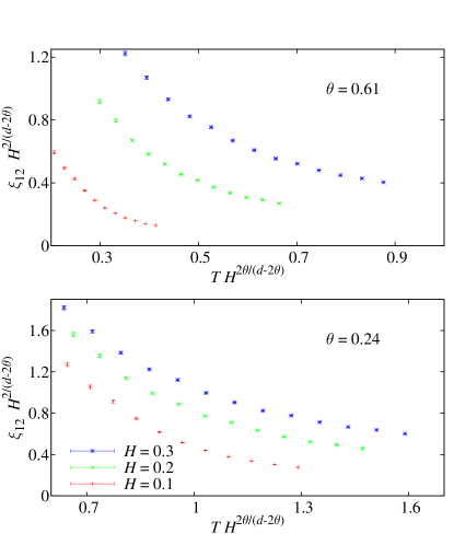
Figure 17: (Color online) Test of the droplet scaling law, Eq. (23). For each of our magnetic fields, we plot $\xi(T,H)\,H^{2/(d-2\theta)}$, as a function of $TH^{2\theta/(d-2\theta)}$. For a proper choice of the stiffness exponent $\theta$, data should collapse in a single curve. We try (and fail within the reachable temperature window) to collapse the data with two different estimates of $\theta$, see Section II.3

VII Conclusions

In this work, we have investigated the approach to equilibrium and the building-up of spin-glass order for the $d=3$ Ising spin glass in an external magnetic field. Specifically, we have simulated the Edwards-Anderson model on the Janus dedicated computer. Our lattices were always much larger ($L=80$) than the correlation length, $\xi(t_{\text{w}})$. Hence, we think that our results are representative of the thermodynamic limit. Our time scales range from the picosecond to one hundredth of a second. We are thus approaching the experimental scale. However, when the temperature was low enough, we have been unable to reach the thermalization time scale, $\tau$. We have monitored this effect carefully. Therefore, in this work we are presenting in a controlled way both equilibrium and non-equilibrium data. Our results have been analyzed on the light of the two major theories on the market, the replica-symmetry breaking and the droplet theory. On the view of recent claims Moore and Drossel (2002); Fullerton and Moore (2013), we have also analyzed our data as suggested by current theories for relaxation in supercooled liquids. None of these three approaches was fully satisfying.

The problem with the droplet/RSB theories was in the correlation length: the growth of $\xi$ upon lowering the temperature is too fast to fit the droplet theory and too slow to fit RSB. We summarize now the strengths and weaknesses of each approach. We start with the droplet theory, then consider RSB and, finally, the supercooled liquids point of view.

As we show in Section VI, the dynamics really seems to be of activated type, as predicted by the droplet theory. However, the scaling law predicted by the theory is not fulfilled by our data. In fact, see Section V.2, the dynamics is of super-Arrhenius type at least down to temperature $T=0.4$ (to be compared with $T_{c}=1.1019(29)$ Baity-Jesi et al. (2013), the $H=0$ critical temperature). Therefore, although the droplet theory might be finally correct at still lower temperature, the corresponding time and length scales would be beyond not only our computational capabilities, but also current experimental possibilities.

The RSB approach resulted in a determination of the de Almeida-Thouless line, which is consistent, whether one uses equilibrium (Section IV) or non-equilibrium (V.1) data. Unfortunately, our equilibrium estimate of $\xi$ does not seem to diverge at the de Almeida-Thouless line (also, the Fisher-Sompolinsky scalingFisher and Sompolinsky (1985) is not verified, as the reader may easily check). There are a number of possible explanations for our failure to find the divergence:

• For all three magnetic fields, we have been able to equilibrate the system only down to $T\approx 1.3T_{\mathrm{c}}(H)$. Perhaps the critical growth of $\xi(T,H)$ starts only closer to the de Almeida-Thouless line.

• It is by no means guaranteed that we are looking at the right correlation function. We have shown in Section VI.1 that some correlators might display sizeable correlations while others do not. In fact, the quest for sensible correlators is a longstanding problem in the investigation of supercooled liquids Franz and Parisi (2000); Kirkpatrick and Thirumalai (1988); Weeks et al. (2000); Berthier et al. (2005); Montanari and Semerjian (2006); Cavagna et al. (2007); Biroli et al. (2008). Also in the field of spin glasses it has been suggested that energy and link-overlap correlators deserve more attention Marinari et al. (1998b); Contucci and Giardinà (2005); Contucci et al. (2006); Alvarez Baños et al. (2010a).

• As explained in Section II.3, it is very possible that the physics in $d=3$ will be ruled by a fixed point at $T=0$. If this is the case, activated dynamics is to be expected also in the RSB theory. Under these circumstances, the de Almeida-Thouless line identified in Section IV and V.1 might well represent a dynamic glass transition. In fact, our data for $\xi(T,H)$ are consistent with a critical divergence below the de Almeida-Thouless line. The divergence could take place in the range $0\leq T_{\mathrm{c}}\leq 0.8$ for $H=0.1$, $0\leq T_{\mathrm{c}}\leq 0.5$ for $H=0.2$ and $0\leq T_{\mathrm{c}}\leq 0.5$ for $H=0.3$ (note, however, that these upper bounds are only crude estimations).

• Finally, as explained above, it is possible that the droplet theory could be correct and no transition takes place for $H>0$ in three spatial dimensions. However, it is clear that the correlation length grows noticeably in our simulations, which suggests that the lower critical dimension in a field cannot be much larger than $d=3$. Notice as well that the lower critical dimension in a field is well below $d=4$, since very clear evidence of a second-order phase transition has been obtained in $d=4$ Baños et al. (2012).

Let us finally consider the supercooled liquid approach. At the qualitative level, this is maybe the most successful description. Indeed, we do identify in our data a Mode Coupling temperature, $T_{\text{d}}$ (Section IV.1) and a cross-over to activated dynamics (Sects. IV.1 and VI.2). However, the description remains qualitative since our numerical accuracy does not allow a strict test of basic relations among critical exponents. We note as well that the would-be Mode Coupling temperature for $H=0.2$, $T_{\mathrm{d}}\approx 1.22$ is rather large as compared to the de Almeida-Thouless line $T_{\mathrm{c}}(H=0.2)\approx 0.7$ (see Section IV). In this respect, we remark that a more typical value for supercooled liquids is $T_{\mathrm{d}}\approx 1.1T_{\mathrm{g}}$ ($T_{\mathrm{g}}$ is the dynamic glass temperature where $\tau\sim$ 1 hour).

We conclude by mentioning that a further finite-size scaling investigation of the problem is now ongoing.

Appendix A Discretization of the Gaussian Magnetic Field

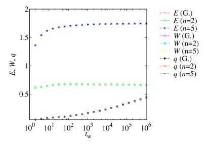
Figure 18: (Color online) Thermal energy $E(t_{\text{w}})$, magnetic energy $W(t_{\text{w}})$ and overlap $q(t_{\text{w}})$ as a function of time for $L=8$, $T=0.7$ and $H=0.3$. We have plotted the results from a full Gaussian distribution (G.), as well as discretizations with $n=2$ and $n=5$. Notice that all three simulations have produced the same equilibrium values for these observables.

In this appendix we describe the procedure we have used to discretize (using the Gauss-Hermite quadrature Abramowitz and Stegun (1972)) the Gaussian magnetic field in order to implement our simulations on the Janus dedicated computer (which cannot handle non-integer arithmetic efficiently). This implementation was introduced (but not explained in detail) in Leuzzi et al. (2009).

The Gauss-Hermite quadrature formula can be interpreted as an approximation formula for probability distributions. In fact, if we multiply either of the two distributions related in Eq. (52), below, by an arbitrary polynomial of order $4n-1$, and integrate this product through $x\in(-\infty,\infty)$, identical results are obtained Abramowitz and Stegun (1972):

$$e^{-x^{2}}\approx\sum_{k=1}^{n}\,\frac{w_{k}}{2}[\delta(x-x_{k})+\delta(x+x_{k})]\,.$$ (52)

where $x_{k}$ are the positive zeros of the $2n$-th Hermite polynomial $H_{2n}(x)$ and the weights, $w_{k}$, are given by

$$w_{k}=\frac{2^{2n-1}(2n)!\sqrt{\pi}}{(2n)^{2}H_{2n-1}(x_{k})^{2}}\,.$$ (53)

In our numerical simulations we need to compute integrals like

$$\overline{O}\equiv\frac{1}{H\sqrt{2\pi}}\int_{-\infty}^{\infty}dh~{}O(h)e^{-\frac{h^{2}}{2H^{2}}}$$ (54)

Furthermore, the above equation can be further simplified using the gauge symmetry (2), which allows us to consider only positive magnetic fields, so

$$\overline{O}=\frac{2}{H\sqrt{2\pi}}\int_{0}^{\infty}dh~{}O(h)e^{-\frac{h^{2}}{2H^{2}}}$$ (55)

and using Eq. (52), one can finally write

$$\overline{O}=\frac{2}{\sqrt{\pi}}\sum_{k=1}^{n}w_{k}O(\sqrt{2}Hx_{k})\,.$$ (56)

We shall limit ourselves to $n=2$ in Eq. (52). Hence, the magnetic field for each site of the lattice is chosen independently: with probability $\tilde{w}_{1}=2w_{1}/\sqrt{\pi}$ the field is $h_{1}=\sqrt{2}Hx_{1}$ (it is set to $h_{2}=\sqrt{2}Hx_{2}$ otherwise). Note that two bits per lattice site are enough to code this $n=2$ approximation, which is very important given the limited memory in Janus. The Gauss-Hermite values for $n=2$ are $x_{1}=0.524647623275$, $x_{2}=1.65068012389$, $w_{1}=0.804914090006$ and $w_{2}=0.0813128354472$ [see Abramowitz and Stegun (1972) or use Eq. (53)].

We have tested numerically the accuracy of the $n=2$-approximation by performing some numerical tests on a small lattice size ($L=8$). Obviously, our $n=2$ approximation should fail for high magnetic fields and small lattice sizes. We have checked that our choice is valid at least for $H\leq 0.3$. In particular, we have compared the results of simulations with $n=2$ (our choice in this work), and $n=5$ with the full Gaussian distribution for the following observables: energy, overlap and $W$(see Figure 18). We have checked that the differences between the observables computed at finite $n$ and those computed with full Gaussian magnetic field are statistically compatible with zero.

Another strong test of our implementation is the agreement in the asymptotic values of $q(t_{\text{w}})$ and $W(t_{\text{w}})$ in the high-temperature phase (see Figure 2).

In conclusion: we have checked that, for the main quantities considered in this work (computed with $n=2$), the systematic error in the approximation (52) is smaller than our statistical accuracy.

Appendix B Spatial correlation functions

In this appendix we discuss three different features of the spatial correlation functions of the $d=3$ spin glass in a magnetic field: (i) the long distance behavior of the replicon correlator (recall Section II.2), (ii) the non-monotonic time behavior in direct quenches (this anomaly seems to be absent from annealing protocols), and (iii) the comparison of the replicon and the longitudinal/anomalous correlators.

B.1 Long-distance behavior of the replicon propagator

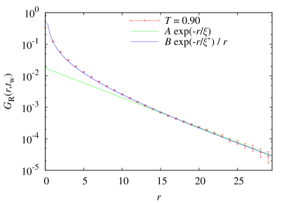
Figure 19: (Color online) Semilogarithmic plot of the equilibrium replicon correlator $G_{\text{R}}$ as a function of distance $r$, for temperature $T=0.9$ and $H=0.2$ [correlations along the lattice direction $(r,0,0)$]. The lines are fits to a single exponential, $G_{\text{R}}(r)\approx A\mathrm{e}^{-r/\xi}$ ($A$ and $\xi$ are fitting parameters), obtained for $r\geq 15$ and to $G_{\text{R}}\approx B\mathrm{e}^{-r/\xi^{\prime}}/r$ for $r\geq 10$. These two functional forms are indistinguishable for large $r$.

As explained in Section II.2, when computing the integrals $I_{k}$, see Eq. (19), it is crucial to impose a long distance cutoff. Otherwise, the $I_{k}$ integrals become non-self-averaging objects that can be accurately computed only with a huge number of samples. However, one may try to correct the systematic effects induced by the cutoff by studying the long-distance behavior of the propagator $G_{\text{R}}$. One fits the curve to a suitable, simple functional form and then computes by hand the remaining part of the integral. The contribution to $I_{k}$ from $r>r_{\text{cutoff}}$ is usually tiny, but we prefer to monitor it. This issue has been discussed at length in Belletti et al. (2008b, 2009a), where the spin glass without a field was studied.

Here, we show in Figure 19 that, in the temperature regime where we manage to equilibrate the system in a field, $G_{\text{R}}(r\gg\xi)$ decays exponentially. Therefore, estimating the contribution from $r>r_{\text{cutoff}}$ to the integrals $I_{k}$ is fairly easy (the resulting correction is smaller than the error bar). We can include an algebraic prefactor in the fitting function the better to fit the small-$r$ sector, but this is irrelevant for the tails (see Figure 19).

B.2 Overshooting in the direct quench

The direct quench is an idealized temperature-variation protocol: one takes a fully disordered spin glass (i.e.. $T=\infty$) and places it instantaneously at the working temperature. It is clear that, in the laboratory, temperature should vary gradually. Hence, the annealing protocols described in Section III.1 are closer to the temperature variations that one can realize experimentally. On the other hand, the direct quench is the simplest protocol in a computer simulation.

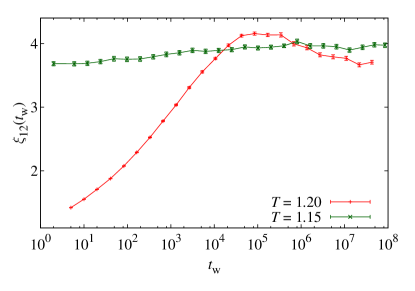
Figure 20: (Color online) Time evolution of the correlation length $\xi_{12}$ as computed for the replicon correlator for temperatures $T=1.2$ and $T=1.15$ in our hot annealing, see Section III.1. Note that the temperature step $T=1.2$ can be regarded as a direct quench, while $T=1.15$ already belongs to the annealing part of the run. The maximum for $T=1.2$, where $\xi_{12}(t_{\text{w}})$ is larger than its equilibrium value, seems to be a generic feature of any direct quench for a spin glass in a field in three dimensions. On the other hand, during the annealing, the time evolution of $\xi_{12}(t_{\text{w}})$ is monotonic.

In fact, we have found with some surprise that the non-equilibrium behavior of the replicon correlator is rather different in a direct quench and in an annealing protocol. In Figure 20 we show the time evolution of the correlation length $\xi_{12}(t_{\text{w}})$ for two temperatures in our hot annealing, the initial one $T=1.2$, and the second temperature $T=1.15$. Note that the time evolution at the very first temperature in the annealing can be aptly described as a direct quench. Indeed, in Figure 20 we notice an overshooting of $\xi(t_{\text{w}})$ in the direct quench: well before equilibrium is reached, a maximum is found which lies above the equilibrium correlation length. No such maximum arises in the lower temperatures of the annealing. We have checked that this overshooting is characteristic of the direct quench, as it happens basically for all temperatures and magnetic fields.

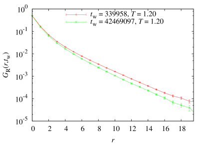
Figure 21: (Color online) Comparison of the non-equilibrium correlator $G_{\text{R}}(r;t_{\text{w}})$ with the corresponding equilibrium value for the initial temperature, $T=1.2$, in our hot annealing (i.e., in a direct quench run). The time $t_{\text{w}}$ corresponds to the maximum correlation length in Figure 20.

We can look at this overshooting in greater detail in Figure 21, where we compare the equilibrium $G_{\text{R}}(r)$ with the non-equilibrium $G_{\text{R}}(r;t_{\text{w}})$ at the $t_{\text{w}}$ corresponding to the maximum in Figure 20. The two correlators are remarkably featureless as a function of $r$, but the overshooting effect is also clear from $G_{\text{R}}(r)$.

B.3 The anomalous/longitudinal sector

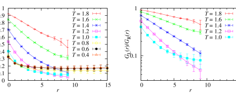
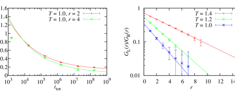
Figure 22: (Color online) Comparison of the replicon and the longitudinal propagator for $H=0.1$. Data from the longest $t_{\text{w}}$ at each temperature step, in our slowest annealing for each temperature. Notational conventions are as in Figure 19. The left panel shows the quotient $G_{\text{L}}/G_{\text{R}}$ for the whole temperature range in a linear scale, while the right panel shows the same quantity in a logarithmic scale (removing the lowest temperatures). In all cases we cut each graph at the point where the statistical error becomes greater than $50\%$. For low $T$, the quotient seems to reach a non-zero asymptotic value. For high temperatures, it seems to decay exponentially, although the decay slows down for large $r$, suggesting a possible non-zero plateau for large $r$.

Figure 23: (Color online) Left: We plot the quotient $G_{\text{L}}/G_{\text{R}}$ for $T=1.0$ and $H=0.1$ as a function of the total time $t_{\text{tot}}$ for two different values of $r$. It is clear that even our longest times have small thermalisation effects. The long-$t_{\text{tot}}$ limit may be estimated with a power-law fit (continuous lines). Right: $G_{\text{L}}/G_{\text{R}}$, extrapolated to infinite $t_{\text{tot}}$ for several temperatures. The curvature observed in Figure 23 has disappeared and a pure exponential decay is now apparent.

The longitudinal/anomalous correlator defined in Eq. (15) appears naturally in the analysis of the mean-field approximation de Almeida and Thouless (1978). To the best of our knowledge, the longitudinal/anomalous correlator has not been studied in three spatial dimensions, in the presence of a field. We recall that from these correlators, one may obtain associated susceptibilities, see Eq. (16).

We showed in Figure 13 that the replicon susceptibility grows significantly upon lowering the temperature, while the longitudinal/anomalous susceptibility does not. However, when looking at the plot of $\chi$, which is a spatial integral of $G$, we are losing information on the shape of the correlation function.

Here we perform a more detailed comparison of both correlators by studying their ratio as a function of $r$ in Fig. 23, left. $G_{\text{L}}/G_{\text{R}}$ was computed at the longest time available, i.e., as close as possible to thermal equilibrium. We identify two different regimes, at high and low temperatures. At high temperatures, $G_{\text{L}}/G_{\text{R}}$ decreases exponentially in $r$, see the right panel in Fig. 23. In fact, barring unavoidable differences on the algebraic prefactors, $G_{\text{L}}(r)/G_{\text{R}}(r)\propto\text{exp}\big{[}-r\,\big{(}\frac{1}{\xi_{\text{L}}}-\frac{1}{\xi_{\text{R}}}\big{)}\big{]}$. Hence the exponential decrease in Fig. 23–right implies $\xi_{\text{R}}>\xi_{\text{L}}$. On the other hand, at the lowest temperatures that we reach, i.e., $T=0.4$ and $0.6$, $G_{\text{L}}/G_{\text{R}}$ becomes essentially constant at large $r$, suggesting that the correlation length is the same for both correlators. This is quite surprising: if a de Almeida-Thouless line exists one expects $0<\xi_{\text{L}}/\xi_{\text{R}}<1$ as we approach it. There is no obvious reason for the two correlation lengths to be equal.

However, the above could be too hasty a conclusion. The reader might be surprised (as we were) by the non-monotonic temperature behavior in the left panel of Fig. 23. One may note that we are mixing thermalized and non-equilibrium data in that figure, which may confuse the situation. An example of the time evolution is shown in the left-panel of Fig. 23. Clearly, at $T=1$ we have still not reached thermal equilibrium within our time scale. Once this is understood, we proceed to extrapolate to infinite time as

$$\frac{G_{\text{L}}(r,t_{\text{tot}})}{G_{\text{R}}(r,t_{\text{tot}})}=\frac{G_{\text{L}}(r,t_{\text{tot}}=\infty)}{G_{\text{R}}(r,t_{\text{tot}}=\infty)}+\frac{A(r)}{t_{\text{tot}}^{x}}\,.$$ (57)

In the above equation, the exponent $x$ was allowed to depend on $r$ and $T$ (we found that it barely depended on $r$ for a given temperature). We were able to carry out this extrapolation safely down to temperature $T=1.0$, see right panel in Fig. 23. In the limit of long times, the ratio of propagators does decrease exponentially with $r$, which confirms that $\xi_{\text{R}}>\xi_{\text{L}}$ (at least down to temperature $T=1.0$, for $H=0.1$ and $H=0.2$, and assuming that the algebraic prefactors in the ratio $G_{L}/G_{R}$ are not relevant).

References

- Debenedetti (1997) P. G. Debenedetti, Metastable Liquids (Princeton University Press, Princeton, 1997).
- Debenedetti and Stillinger (2001) P. G. Debenedetti and F. H. Stillinger, Nature 410, 259 (2001).
- Cavagna (2009) A. Cavagna, Physics Reports 476, 51 (2009), arXiv:0903.4264 .
- Mydosh (1993) J. A. Mydosh, Spin Glasses: an Experimental Introduction (Taylor and Francis, London, 1993).
- Montanari and Semerjian (2006) A. Montanari and G. Semerjian, J. Stat. Phys. 125, 23 (2006), arXiv:cond-mat/0201107 .
- Adam and Gibbs (1965) G. Adam and J. H. Gibbs, J. Chem. Phys. 43, 139 (1965).
- Weeks et al. (2000) E. R. Weeks, J. C. Crocker, A. C. Levitt, A. Schofield, and D. A. Weitz, Science 287, 627 (2000).
- Berthier et al. (2005) L. Berthier, G. Biroli, J.-P. Bouchaud, L. Cipelletti, D. El Masri, D. L’Hôte, F. Ladieu, and M. Pierno, Science 310, 1797 (2005).
- Gunnarsson et al. (1991) K. Gunnarsson, P. Svedlindh, P. Nordblad, L. Lundgren, H. Aruga, and A. Ito, Phys. Rev. B 43, 8199 (1991).
- Palassini and Caracciolo (1999) M. Palassini and S. Caracciolo, Phys. Rev. Lett. 82, 5128 (1999), arXiv:cond-mat/9904246 .
- Ballesteros et al. (2000) H. G. Ballesteros, A. Cruz, L. A. Fernandez, V. Martin-Mayor, J. Pech, J. J. Ruiz-Lorenzo, A. Tarancon, P. Tellez, C. L. Ullod, and C. Ungil, Phys. Rev. B 62, 14237 (2000), arXiv:cond-mat/0006211 .
- Hérisson and Ocio (2002) D. Hérisson and M. Ocio, Phys. Rev. Lett. 88, 257202 (2002), arXiv:cond-mat/0112378 .
- Joh et al. (1999) Y. G. Joh, R. Orbach, G. G. Wood, J. Hammann, and E. Vincent, Phys. Rev. Lett. 82, 438 (1999).
- Bert et al. (2004) F. Bert, V. Dupuis, E. Vincent, J. Hammann, and J.-P. Bouchaud, Phys. Rev. Lett. 92, 167203 (2004).
- Cruz et al. (2001) A. Cruz, J. Pech, A. Tarancon, P. Tellez, C. L. Ullod, and C. Ungil, Comp. Phys. Comm 133, 165 (2001), arXiv:cond-mat/0004080 .
- Ogielski (1985) A. T. Ogielski, Phys. Rev. B 32, 7384 (1985).
- Belletti et al. (2006) F. Belletti, F. Mantovani, G. Poli, S. F. Schifano, R. Tripiccione, I. Campos, A. Cruz, D. Navarro, S. Perez-Gaviro, D. Sciretti, A. Tarancon, J. L. Velasco, P. Tellez, L. A. Fernandez, V. Martin-Mayor, A. Muñoz Sudupe, S. Jimenez, A. Maiorano, E. Marinari, and J. J. Ruiz-Lorenzo (Janus Collaboration), Computing in Science and Engineering 8, 41 (2006).
- Belletti et al. (2008a) F. Belletti, M. Cotallo, A. Cruz, L. A. Fernandez, A. Gordillo, A. Maiorano, F. Mantovani, E. Marinari, V. Martin-Mayor, A. Muñoz Sudupe, D. Navarro, S. Perez-Gaviro, J. J. Ruiz-Lorenzo, S. F. Schifano, D. Sciretti, A. Tarancon, R. Tripiccione, and J. L. Velasco (Janus Collaboration), Comp. Phys. Comm. 178, 208 (2008a), arXiv:0704.3573 .
- Belletti et al. (2008b) F. Belletti, M. Cotallo, A. Cruz, L. A. Fernandez, A. Gordillo-Guerrero, M. Guidetti, A. Maiorano, F. Mantovani, E. Marinari, V. Martin-Mayor, A. M. Sudupe, D. Navarro, G. Parisi, S. Perez-Gaviro, J. J. Ruiz-Lorenzo, S. F. Schifano, D. Sciretti, A. Tarancon, R. Tripiccione, J. L. Velasco, and D. Yllanes (Janus Collaboration), Phys. Rev. Lett. 101, 157201 (2008b), arXiv:0804.1471 .
- Belletti et al. (2009a) F. Belletti, A. Cruz, L. A. Fernandez, A. Gordillo-Guerrero, M. Guidetti, A. Maiorano, F. Mantovani, E. Marinari, V. Martin-Mayor, J. Monforte, A. Muñoz Sudupe, D. Navarro, G. Parisi, S. Perez-Gaviro, J. J. Ruiz-Lorenzo, S. F. Schifano, D. Sciretti, A. Tarancon, R. Tripiccione, and D. Yllanes (Janus Collaboration), J. Stat. Phys. 135, 1121 (2009a), arXiv:0811.2864 .
- Alvarez Baños et al. (2010a) R. Alvarez Baños, A. Cruz, L. A. Fernandez, J. M. Gil-Narvion, A. Gordillo-Guerrero, M. Guidetti, A. Maiorano, F. Mantovani, E. Marinari, V. Martin-Mayor, J. Monforte-Garcia, A. Muñoz Sudupe, D. Navarro, G. Parisi, S. Perez-Gaviro, J. J. Ruiz-Lorenzo, S. F. Schifano, B. Seoane, A. Tarancon, R. Tripiccione, and D. Yllanes (Janus Collaboration), J. Stat. Mech. 2010, P06026 (2010a), arXiv:1003.2569 .
- Alvarez Baños et al. (2010b) R. Alvarez Baños, A. Cruz, L. A. Fernandez, J. M. Gil-Narvion, A. Gordillo-Guerrero, M. Guidetti, A. Maiorano, F. Mantovani, E. Marinari, V. Martin-Mayor, J. Monforte-Garcia, A. Muñoz Sudupe, D. Navarro, G. Parisi, S. Perez-Gaviro, J. J. Ruiz-Lorenzo, S. F. Schifano, B. Seoane, A. Tarancon, R. Tripiccione, and D. Yllanes (Janus Collaboration), Phys. Rev. Lett. 105, 177202 (2010b), arXiv:1003.2943 .
- Franz et al. (1998) S. Franz, M. Mézard, G. Parisi, and L. Peliti, Phys. Rev. Lett. 81, 1758 (1998).
- de Almeida and Thouless (1978) J. R. L. de Almeida and D. J. Thouless, J. Phys. A 11, 983 (1978).
- Mézard et al. (1987) M. Mézard, G. Parisi, and M. Virasoro, Spin-Glass Theory and Beyond (World Scientific, Singapore, 1987).
- Marinari et al. (2000) E. Marinari, G. Parisi, F. Ricci-Tersenghi, J. J. Ruiz-Lorenzo, and F. Zuliani, J. Stat. Phys. 98, 973 (2000), arXiv:cond-mat/9906076 .
- Moore and Drossel (2002) M. A. Moore and B. Drossel, Phys. Rev. Lett. 89, 217202 (2002), arXiv:cond-mat/0201107 .
- Fullerton and Moore (2013) C. J. Fullerton and M. A. Moore, (2013), arXiv:1304.4420 .
- Kirkpatrick and Thirumalai (1987) T. R. Kirkpatrick and D. Thirumalai, Phys. Rev. B 36, 5388 (1987).
- Kirkpatrick et al. (1989) T. R. Kirkpatrick, D. Thirumalai, and P. G. Wolynes, Phys. Rev. A 40, 1045 (1989).
- Götze and Sjögren (1992) W. Götze and T. F. Sjögren, Rep. Prog. Phys. 55, 241 (1992).
- Mézard and Parisi (1999a) M. Mézard and G. Parisi, Phys. Rev. Lett. 82, 747 (1999a).
- Mézard and Parisi (1999b) M. Mézard and G. Parisi, J. Chem. Phys. 111, 1076 (1999b).
- Coluzzi et al. (2000) B. Coluzzi, G. Parisi, and P. Verrocchio, Phys. Rev. Lett. 84, 306 (2000).
- Parisi and Rizzo (2010) G. Parisi and T. Rizzo, J. Phys. A 43, 235003 (2010).
- Singh et al. (2013) S. Singh, M. Ediger, and J. de Pablo, Nature Mater. 12, 139 (2013).
- McMillan (1984) W. L. McMillan, J. Phys. C: Solid State Phys. 17, 3179 (1984).
- Bray and Moore (1987) A. J. Bray and M. A. Moore, in Heidelberg Colloquium on Glassy Dynamics, Lecture Notes in Physics No. 275, edited by J. L. van Hemmen and I. Morgenstern (Springer, Berlin, 1987).
- Fisher and Huse (1986) D. S. Fisher and D. A. Huse, Phys. Rev. Lett. 56, 1601 (1986).
- Fisher and Huse (1988) D. S. Fisher and D. A. Huse, Phys. Rev. B 38, 386 (1988).
- Moore and Bray (2011) M. A. Moore and A. J. Bray, Phys. Rev. B 83, 224408 (2011), arXiv:1102.1675 .
- Parisi and Temesvári (2012) G. Parisi and T. Temesvári, Nucl. Phys. B 858, 293 (2012), arXiv:1111.3313 .
- Yeo and Moore (2012) J. Yeo and M. A. Moore, Phys. Rev. E 86, 052501 (2012), arXiv:1208.3044 .
- Young and Katzgraber (2004) A. P. Young and H. G. Katzgraber, Phys. Rev. Lett. 93, 207203 (2004), arXiv:cond-mat/0407031 .
- Jörg et al. (2008) T. Jörg, H. G. Katzgraber, and F. Krzakala, Phys. Rev. Lett. 100, 197202 (2008), arXiv:0712.2009 .
- Jönsson et al. (2005) P. E. Jönsson, H. Takayama, H. A. Katori, and A. Ito, Phys. Rev. B 71, 180412(R) (2005), arXiv:cond-mat/0411291 .
- Petit et al. (1999) D. Petit, L. Fruchter, and I. A. Campbell, Phys. Rev. Lett 83, 5130 (1999), arXiv:cond-mat/9910353 .
- Petit et al. (2002) D. Petit, L. Fruchter, and I. A. Campbell, Phys. Rev. Lett 88, 207206 (2002), arXiv:cond-mat/011112 .
- Tabata et al. (2010) Y. Tabata, K. Matsuda, S. Kanada, T. Yamazaki, T. Waki, H. Nakamura, K. Sato, and K. Kindo, Journal of Physical Society of Japan 79, 123704 (2010), arXiv:1009.6115 .
- Baños et al. (2012) R. A. Baños, A. Cruz, L. A. Fernandez, J. M. Gil-Narvion, A. Gordillo-Guerrero, M. Guidetti, D. Iniguez, A. Maiorano, E. Marinari, V. Martin-Mayor, J. Monforte-Garcia, A. Muñoz Sudupe, D. Navarro, G. Parisi, S. Perez-Gaviro, J. J. Ruiz-Lorenzo, S. F. Schifano, B. Seoane, A. Tarancon, P. Tellez, R. Tripiccione, and D. Yllanes, Proc. Natl. Acad. Sci. USA 109, 6452 (2012).
- Kotliar et al. (1983) G. Kotliar, P. W. Anderson, and D. L. Stein, Phys. Rev. B 27, 602 (1983).
- Larson et al. (2013) D. Larson, H. G. Katzgraber, M. A. Moore, and A. P. Young, Phys. Rev. B 87, 024414 (2013), arXiv:1211.7297 .
- Leuzzi and Parisi (2013) L. Leuzzi and G. Parisi, Phys. Rev. B 88, 224204 (2013), arXiv:1303.6333 .
- de Dominicis and Giardina (2006) C. de Dominicis and I. Giardina, Random Fields and Spin Glasses (Cambridge University Press, Cambridge, England, 2006).
- Parisi (1994) G. Parisi, Field Theory, Disorder and Simulations (World Scientific, 1994).
- Belletti et al. (2009b) F. Belletti, M. Guidetti, A. Maiorano, F. Mantovani, S. F. Schifano, R. Tripiccione, M. Cotallo, S. Perez-Gaviro, D. Sciretti, J. L. Velasco, A. Cruz, D. Navarro, A. Tarancon, L. A. Fernandez, V. Martin-Mayor, A. Muñoz-Sudupe, D. Yllanes, A. Gordillo-Guerrero, J. J. Ruiz-Lorenzo, E. Marinari, G. Parisi, M. Rossi, and G. Zanier (Janus Collaboration), Computing in Science and Engineering 11, 48 (2009b).
- Baity-Jesi et al. (2012) M. Baity-Jesi, R. A. Baños, A. Cruz, L. A. Fernandez, J. M. Gil-Narvion, A. Gordillo-Guerrero, M. Guidetti, D. Iniguez, A. Maiorano, F. Mantovani, E. Marinari, V. Martin-Mayor, J. Monforte-Garcia, A. Munoz Sudupe, D. Navarro, G. Parisi, M. Pivanti, S. Perez-Gaviro, F. Ricci-Tersenghi, J. J. Ruiz-Lorenzo, S. F. Schifano, B. Seoane, A. Tarancon, P. Tellez, R. Tripiccione, and D. Yllanes, Eur. Phys. J. Special Topics 210, 33 (2012), arXiv:1204.4134 .
- Abramowitz and Stegun (1972) M. Abramowitz and I. A. Stegun, Handbook of Mathematical Functions: with Formulas, Graphs, and Mathematical Tables., ninth ed. (Dover Publications, New York, 1972).
- Bray and Roberts (1980) A. J. Bray and S. A. Roberts, J. Phys. C: Solid St.Phys. 13, 5405 (1980).
- Fisher and Sompolinsky (1985) D. S. Fisher and H. Sompolinsky, Phys. Rev. Lett. 54, 1063 (1985).
- Temesvári and De Dominicis (2002) T. Temesvári and C. De Dominicis, Phys. Rev. Lett. 89, 097204 (2002), arXiv:cond-mat/0207512 .
- Temesvári (2008) T. Temesvári, Phys. Rev. B 78, 220401 (2008).
- Hartmann (1999) A. K. Hartmann, Phys. Rev. E. 59, 84 (1999), arXiv:cond-mat/9806114 .
- Palassini and Young (1999) M. Palassini and A. P. Young, Phys. Rev. Lett. 83, 5126 (1999).
- Boettcher (2004) S. Boettcher, Eur. Phys. J. B 38, 83 (2004), arXiv:cond-mat/0310698 .
- Palassini and Young (2000) M. Palassini and A. P. Young, Phys. Rev. Lett. 85, 3017 (2000).
- Krzakala and Martin (2000) F. Krzakala and O. C. Martin, Phys. Rev. Lett. 85, 3013 (2000).
- Yllanes (2011) D. Yllanes, Rugged Free-Energy Landscapes in Disordered Spin Systems (Ph.D. thesis, UCM, 2011) arXiv:1111.0266 .
- Sompolinsky and Zippelius (1982) H. Sompolinsky and A. Zippelius, Phys. Rev. B 25, 6860 (1982).
- Nattermann (1998) T. Nattermann, in Spin glasses and random fields, edited by A. P. Young (World Scientific, Singapore, 1998).
- Götze (2009) W. Götze, Complex dynamics of glass-forming liquids: A mode-coupling theory (Oxford University Press, USA, 2009).
- Andreanov et al. (2009) A. Andreanov, G. Biroli, and J.-P. Bouchaud, Europhysics Letters 88, 16001 (2009).
- Franz et al. (2012a) S. Franz, H. Jacquin, G. Parisi, P. Urbani, and F. Zamponi, J. Chem. Phys. 138, 12A540 (2012a), arXiv:1210.7304 .
- Franz et al. (2012b) S. Franz, H. Jacquin, G. Parisi, P. Urbani, and F. Zamponi, Proc. Natl. Acad. Sci. USA 109, 18725 (2012b), arXiv:1206.2482 .
- Caltagirone et al. (2012) F. Caltagirone, U. Ferrari, L. Leuzzi, G. Parisi, F. Ricci-Tersenghi, and T. Rizzo, Phys. Rev. Lett. 108, 085702 (2012), arXiv:1111.6420 .
- Kob and Andersen (1994) W. Kob and H. C. Andersen, Phys. Rev. Lett. 73, 1376 (1994).
- Lubchenko and Wolynes (2007) V. Lubchenko and P. G. Wolynes, Annu. Rev. Phys. Chem. 58, 235 (2007).
- Jonsson et al. (1999) T. Jonsson, K. Jonason, P. E. Jönsson, and P. Nordblad, Phys. Rev. B 59, 8770 (1999).
- Parisi et al. (1998) G. Parisi, F. Ricci-Tersenghi, and J. J. Ruiz-Lorenzo, Phys. Rev. B 57, 13617 (1998), arXiv:cond-mat/9711122 .
- Marinari et al. (1998a) E. Marinari, G. Parisi, and F. Zuliani, J. Phys. A: Math. and Gen. 31, 1181 (1998a), arXiv:cond-mat/9703253 .
- Note (1) can be expressed as: , where is the dimensionality of the system, is the dynamical critical exponent and is the anomalous dimension.
- Baity-Jesi et al. (2013) M. Baity-Jesi, R. A. Baños, A. Cruz, L. A. Fernandez, J. M. Gil-Narvion, A. Gordillo-Guerrero, D. Iniguez, A. Maiorano, F. Mantovani, E. Marinari, V. Martin-Mayor, J. Monforte-Garcia, A. Muñoz Sudupe, D. Navarro, G. Parisi, S. Perez-Gaviro, M. Pivanti, F. Ricci-Tersenghi, J. J. Ruiz-Lorenzo, S. F. Schifano, B. Seoane, A. Tarancon, R. Tripiccione, and D. Yllanes (Janus Collaboration), Phys. Rev. B 88, 224416 (2013), arXiv:1310.2910 .
- Franz and Parisi (2000) S. Franz and G. Parisi, J. of Physics: Condensed Matter 12, 6335 (2000).
- Kirkpatrick and Thirumalai (1988) T. R. Kirkpatrick and D. Thirumalai, Phys. Rev. A 37, 4439 (1988).
- Cavagna et al. (2007) A. Cavagna, T. S. Grigera, and P. Verrocchio, Phy. Rev. Lett. 98, 187801 (2007), arXiv:cond-mat/0607817 .
- Biroli et al. (2008) G. B. J. P. Biroli, A. Cavagna, T. S. Grigera, and P. Verrocchio, Nature Physics 4, 771 (2008), arXiv:cond-mat/0607817 .
- Marinari et al. (1998b) E. Marinari, G. Parisi, and J. J. Ruiz-Lorenzo, Phys. Rev. B 58, 14852 (1998b).
- Contucci and Giardinà (2005) P. Contucci and C. Giardinà, Phys. Rev. B 72, 014456 (2005).
- Contucci et al. (2006) P. Contucci, C. Giardinà, C. Giberti, and C. Vernia, Phys. Rev. Lett. 96, 217204 (2006).
- Leuzzi et al. (2009) L. Leuzzi, G. Parisi, F. Ricci-Tersenghi, and J. J. Ruiz-Lorenzo, Phys. Rev. Lett. 103, 267201 (2009), arXiv:0811.3435 .