Abstract

We developed an automated pattern recognition code that is particularly well suited to extract one-dimensional curvi-linear features from two-dimensional digital images. A former version of this Oriented Coronal CUrved Loop Tracing (OCCULT) code was applied to spacecraft images of magnetic loops in the solar corona, recorded with the NASA spacecraft Transition Region And Coronal Explorer (TRACE) in extreme ultra-violet wavelengths. Here we apply an advanced version of this code (OCCULT-2) also to similar images from the Solar Dynamics Observatory (SDO), to chromospheric H-$\alpha$ images obtained with the Swedish Solar Telescope (SST), and to microscopy images of microtubule filaments in live cells in biophysics. We provide a full analytical description of the code, optimize the control parameters, and compare the automated tracing with visual/manual methods. The traced structures differ by up to 16 orders of magnitude in size, which demonstrates the universality of the tracing algorithm.

10.3390/—— xx Received: xx / Accepted: xx / Published: xx Optimization of Curvi-Linear Tracing Applied to Solar Physics and Biophysics Markus J. Aschwanden ^1∗, Bart De Pontieu ¹, and Eugene A. Katrukha ² aschwanden@lmsal.com, Phone: 650-424-4001, Fax: 650-424-3994.

1 Introduction

Image segmentation is an image processing method that subdivides an image into its constituent regions or objects, which can have the one-dimensional geometry of curvi-linear (1D) segments, or the two-dimensional (2D) geometry of (fractal) areas. Common techniques include point, line, and edge detection, edge linking and boundary detection, Hough transform, thresholding, region-based segmentation, morphological watersheds, etc. (e.g., gonzales2008 ). Since there exists no omni-potent automated pattern recognition code that works for all types of images equally well, we have to customize suitable algorithms for each data type individually by taking advantage of the particular geometry of the features of interest, using a priori information from the data. In this study we optimize an automated pattern recognition code to extract magnetized loops from images of the solar corona with the aim of optimum completeness and fidelity. We will demonstrate that the same code works also equally well for microscopic images in biophysics. The particular geometric property of the extracted features is the relatively large curvature radius of coronal magnetic field lines, which generally do not have sharp kinks and corners, but exhibit continuity in the variation of the local curvature radius along their length. Using a related strategy of curvature constraints, coronal loops were extracted also with the directional 2D Morlet wavelet transform (biskri2010 ). In addition, solar coronal loops, as well as biological microtubule filaments, have a relatively small cross-section compared with their length, so that they can be treated as curvi-linear 1D objects in a tracing method. Tracing of 1D structures with large curvature radii simplifies an automated algorithm enormously, compared with segmentation of 2D regions with arbitrary geometry and possibly fractal fine structure mcateer2005 .

The content of this paper includes a brief description of the automated tracing code (Section 2), applications to images in solar physics (Section 3), to images in biophysics (Section 4), discussion and conclusions (Section 5), and a full analytical description of the code in Appendix A.

2 Description of the Automated Tracing Code

Early versions of Oriented-Connectivity Methods (OCM) applied to solar images were pioneered by Lee, Newman, and Gary lee2004 ; lee2006 . This code was applied to a Transition Region And Coronal Explorer (TRACE) image and a total of 57 coronal loops were detected in a solar active region, which supposedly outline the dipolar magnetic field. The results of this code were compared among five numerical codes based on similar curvi-linear loop-segmentation methods in a study of Aschwanden aschwanden2008 , in terms of the cumulative size distribution of loop lengths, the median and maximum detected loop lengths, the completeness and detection efficiency, accuracy, and flux sensitivity. One of these codes was developed further, which we call Oriented Coronal CUrved Loop Tracing (OCCULT) code, and was found to approach the quality of visually and manually traced loops, detecting a total of 272 loop structures in the same TRACE image aschwanden2010 . In the study here we developed this code further and tested it in a larger parameter space and with different types of images. Technical details of the original OCCULT code are given in aschwanden2010 , a concise description of the advanced OCCULT-2 code is given in the following, while a comprehensive analytical description of OCCULT-2 is provided in Appendix A.

1. Background supression: The median $z_{med}$ of an intensity image $z_{ij}=I_{0}(x_{i},y_{i})$ is computed, and the low intensity values with $z_{ij}<z_{min}$ are set to the base value $z_{min}=z_{med}\times q_{med}$, with $q_{med}$ being a selectable control parameter, with a default value $q_{med}=1.0$ if applied, and $q_{med}=0$ if ignored, while a range of $1\lower 1.72218pt\hbox{$\;\buildrel<\over{\scriptstyle\sim}\;$}q_{med}\lower 1.72218pt\hbox{$\;\buildrel<\over{\scriptstyle\sim}\;$}2.5$ was found to be useful for noisy data. The median value $z_{med}$ is a good estimate of the background (if the features of interest cover less than 50% of the image area) and can manually be adjusted with the multiplier $q_{med}$ otherwise. The parts of the original image that have intensities below this base level, are then rendered with a constant value, are noise-free, and will automatically suppress any structure detection in the background below this base level. This new method is more flexible and efficient in suppressing faint background structures.

2. Highpass and lowpass filtering: A lowpass filter with a boxcar smoothing constant $n_{sm1}$ smoothes out the data noise (e.g., photon noise with Poisson statistics in astrophysical and microscopy images, e.g., see pawley2008 ), while a highpass filter with a boxcar smoothing constant $n_{sm2}$ enhances the fine structure. The two combined filters represent a bandpass filter (with $n_{sm1}<n_{sm2}$), defined by

   $$I^{filter}(x_{i},y_{j})=smooth[I_{0}(x_{i},y_{j}),n_{sm1}]-smooth[I_{0}(x_{i},y_{j}),n_{sm2}]\ .$$ (1)

   For theoretical and experimental reasons, a filter combination of $n_{sm2}=n_{sm1}+2$ yields the sharpest enhancement of the intermediate spatial scale, and thus warrants optimum performance in tracing of curvi-linear structures.

3. Initialization of loop structures: The code initializes the first structure to be traced from the position $(x_{0}^{a},y_{0}^{a})$ with the maximum brightness or flux intensity $f_{0}^{a}=I_{0}(x_{0}^{a},y_{0}^{a})$ in the original image $I_{0}(x,y)$. Once the full loop has been traced, the area of the detected loop is erased to zero, and the next loop structure is initialized at the position $(x_{0}^{b},y_{0}^{b})$ with the next flux maximum $f_{0}^{b}$ in the residual image. The initialization of subsequent loops $(f_{0}^{c},f_{0}^{d},...)$ is continued iteratively until the residual image becomes entirely zeroed out, the increase of detected structures stagnates, or a maximum loop number $N_{max}$ is reached.

4. Loop structure tracing: An initialized structure starting at its flux maximum position $(x_{0},y_{0})$ is then traced in forward direction to the first end point of the loop, and then in opposite direction from the original starting point to the second endpoint. The two bi-directional segments are then combined into a single uni-directional 1D path $s_{i}=s(x_{i},y_{i})$, $i=1,...,n_{s}$. The step-wise tracing along a loop structure position $s_{i}$ is carried out by determining first the direction of the local ridge (defined by the azimuthal angle $\alpha_{l}$ with respect to the $x$-axis), and secondly by determining the local curvature radius $r_{m}$. The curved segment that follows a local ridge closest, is used as a second-order polynomial to extrapolate the traced loop segment by one incremental step (of $\Delta s=1$ pixel). This second-order guiding criterion represents an improvement over the first-order guiding criterion used in the previous OCCULT code aschwanden2010 . The second-order guiding criterion is defined by the brightness distribution $f(s)=f[x_{seg}(s),y_{seg}(s)]$ along a loop segment with constant curvature radius and length $n_{s}$. If the segment follows an ideal ridge with a constant curvature radius and a constant brightness, the summed (or averaged) flux along the ridge segment has a maximum value, while it exhibits a minimum in perpendicular direction to the ridge, where the brightness profile collapes to a $\delta$-function.

5. Loop subtraction in residual image: Once a full loop structure has been traced, the loop area $I_{0}(x_{i}\pm w,y_{j}\pm w)$, $i=1,...,n_{s}$, is set to zero within a half width of $w=(n_{sm2}/2-1)$, so that the area of a former detected loop is not used in the detection of subsequent loops. However, crossing loops can still be connected over a gap.

The original automated loop tracing code (OCCULT) employed the following control parameters: the highpass filter boxcar $n_{sm2}$, the noise threshold level $N_{\sigma}$, the minimum curvature radius $r_{min}$, the moving segment length $n_{s}$, the directional angle range $\Delta\alpha$, and a filling factor $q_{fill}$ for the guiding criteron. In the advanced code (OCCULT-2) we use only two free parameters: the lowpass filter $n_{sm1}$, and the minimum curvature radius $r_{min}$. In addition, noise treatment is handled by selecting a typical noise area in the image, as well as the control factor $q_{med}$ that ignores faint structures below the base level $z_{min}=z_{med}\times q_{med}$. Thus, the new version of the code offers a simpler choice of control parameters for automated detection of structures.

3 Application to Solar Physics

In the following three subsections we process three different types of solar images, one from the TRACE spacecraft (Section 3.1), one from the SDO spacecraft (Section 3.2), and one from a ground-based solar telescope (Section 3.3). Some parameters of the analyzed images are listed in Table 1.

Table 1: Parameters of five analyzed images, including the range of brightness in the image ($z_{min},z_{max}$), the minimum curvature radius $r_{min}$ (in units of pixels), the bandpass filter ($n_{sm1},n_{sm2}$), the total number of detected loops $N_{det}(L>30)$, the number of detected long loops $N_{det}(L>70)$, and the powerlaw slope of the cumulative length distribution $p_{L}$.

Image	Brightness	Minimum	Filter	Number of	Number of	Powerlaw
	range	curvature	range	all loops	long loops	slope
	$z_{min},z_{max}$	$r_{min}$	$n_{sm1},n_{sm2}$	$N_{det}(L>30)$	$N_{det}(L>70)$	$p_{L}$
TRACE	56, 2606	30	5, 7	437	134	3.1
SDO/AIA	28, 255	30	9, 11	503	121	2.7
SST	339, 916	30	3, 5	1757	376	3.9
Cell-HC	416, 65535	15	3, 5	208	51	3.1
Cell-LC	289, 18699	30	7, 9	151	39	2.7

3.1 TRACE Data

The first image we are processing has been used as a standard in a number of previous publications lee2004 ; lee2006 ; aschwanden2008 ; aschwanden2010 , which shows coronal loops in a dipolar active region that was recorded by the TRACE spacecraft on 1998 May 5, 22:21 UT, in the 171 Å wavelength (Fig. 1, center). The original image has a size of $1024\times 1024$ pixels with a pixelsize of 0.5^′′($\approx 360$ km on the solar surface). The EUV brightness or intensity in every pixel is quantified by a data number (DN), which has a minimum of 56 DN and a maximum of 2606 DN in this image. We show the bandpass-filtered image (with a lowpass boxcar of $n_{sm1}=5$ pixels and a highpass boxcar of $n_{sm2}=7$ pixels) in Fig. 2. The image shows at least four different textures (Fig. 1, side panels): coronal loops (L: curvi-linear features), so-called moss regions (M: high-constrast reticulated or spongy features in the center of the image, which represent the footpoints of hot coronal loops), transition region emission (T: low-contrast irregular features in the background), and faint emission areas. The faint image areas show in addition a ripple with diagonal stripes at a pedestal level of $\approx 57\pm 1$ DN (Fig. 2 bottom left panel R) that results from some interference in the electronic readout, which can produce unwanted non-solar structures in the automated detection of curvi-linear features.

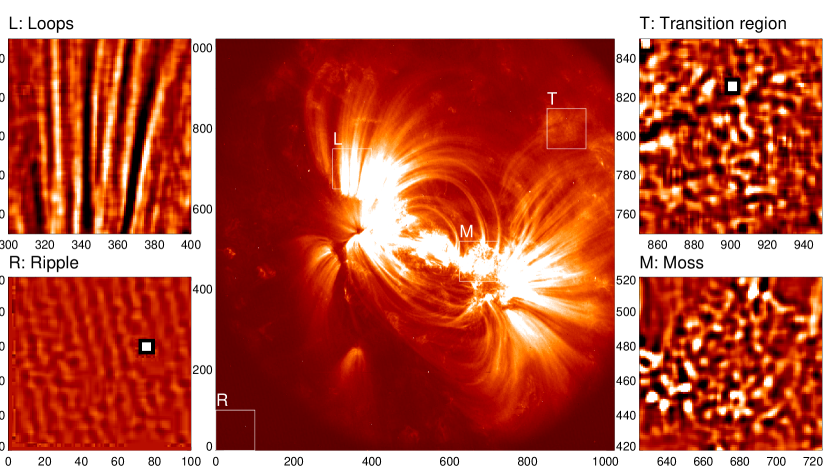
Figure 1: A solar EUV image of an active region, recorded with the TRACE spacecraft on 1998 May 15, is shown with a colorscale that has the highest brightness in the white regions (center). In addition we show ($100\times 100$ pixel) enlargements of four subregions with different textures, which contain coronal loops (top left panel), electronic ripple (bottom left panel), chromospheric and transition region emission (top right panel), and moss regions with footpoints of hot coronal loops (bottom right panel).

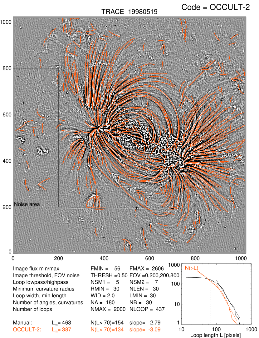
Figure 2: A bandpass-filtered ($n_{sm1}=5,n_{sm2}=7$) version of the original image rendered in Fig. 1 is shown (greyscale), with automated loop tracings overlaid (red curves). Cumulative size distributions $N(>L)$ of loop lengths are also shown (bottom right panel), comparing the automated tracing (red distribution) with visually/manually traced loops (black distribution). The maximum lengths $L_{m}$ (in pixels) are listed for the longest loops detected with each method.

The automated detection of curvi-linear features with the OCCULT-2 code yields a total of 437 loop structures with lengths of $L\geq 30$ pixels (Fig. 2), whereof the longer loops (with lengths of $L\lower 1.72218pt\hbox{$\;\buildrel>\over{\scriptstyle\sim}\;$}50$) coincide well with the 210 visually/manually traced loops (see Fig.7 in aschwanden2010 ). The good agreement between the automated and visually detected loops can also be seen from the cumulative size distributions of loop lengths obtained with both methods (Fig. 1, bottom right panel). The two methods detect $N=154$ and $N=134$ loops with a length of $L\geq 70$ pixels, and both distributions have a powerlaw slope of $\alpha_{L}\approx 2.9\pm 0.1$. Challenges of coronal loop detection in this image are confusion and interference from all three types of non-loop structures (Fig. 1): chains of ”dotted moss structures”, filamentary and spicular transition region emission, and the diagonal stripes of electronic ripple in the background, which become all comparable with the signal of loop structures once the image contrast is enhanced with a highpass filter.

Figure 3: The optimization of the highpass filter constant $n_{sm2}$ (y-axis) is shown for the number of detected loops (with lengths longer than 70 pixels) for all analyzed cases, $N_{det}(L\geq 70)$ (left panels). The optimization of detected loops as a function of the curvature radius $r_{min}$ is also shown (right panels).

The successful or false detection in an image thus depends most strongly on the chosen low and highpass filter constant $n_{sm2}$ and the background base level $z_{min}=z_{med}\times q_{med}$, and to a lesser degree on the other control parameters. A good indicator of the completeness and efficiency of automated loop detection is the number of coherently detected long loops, say with a length above 70 pixels here, $N_{det}(L>70)$ (which is marked with a dotted line in the size distribution in Fig. 2, bottom right panel). In Fig. 3 (top left panel) we show how this detection efficiency $N_{det}(n_{sm2})$ varies as a function of the chosen control parameter $n_{sm2}$. The detected number has a maximum of $N_{det}=134$ at $n_{smi1}=5$ and $n_{sm2}=7$, which corresponds to a bandpass filter in the range of 5-7 pixels ($2.5\hbox{${}^{\prime\prime}$}-3.5\hbox{${}^{\prime\prime}$}$ or 1800-2500 km on the solar surface). It appears that this is the most typical cross-section width (FWHM) of coronal loops. Other statistical studies of coronal loops observed with TRACE yield similar values (e.g., FWHM=$1420\pm 340$ km; aschwanden2005 ). Thus, if an image contains structures with a preferential cross-section width, the relevant cross-section range can be bracketed with a bandpass filter ($n_{sm1},n_{sm2}$), providing a useful a priori information for automated detection of curvi-linear features. We conducted tests with all possible filter widths $n_{sm1}=1,3,...,21$ and $n_{sm2}>n_{sm1}$ and found that the largest number of detected structures virtually always occurs at $n_{sm2}=n_{sm1}+2$, which can be explained also by the theoretical argument that the best signal-to-noise ratio is obtained for maximum smoothing of the highpass-filtered (unsharp mask) image. We vary also the minimum curvature radius $r_{min}$ and find a maximum of detected structures at $r_{min}\approx 30$ pixels (Fig. 3 top right panel).

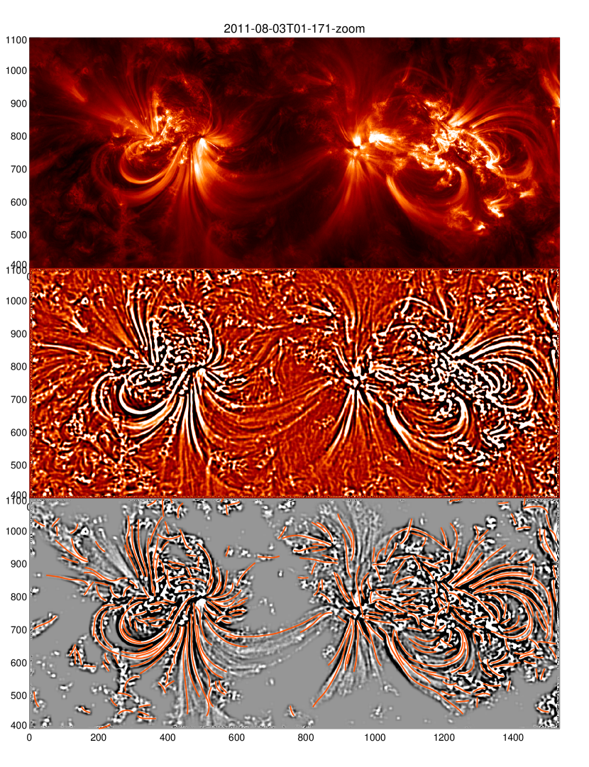
Figure 4: Bandpass-filtered image of an active region complex observed with AIA/SDO on 2011 Aug 3, 01 UT, 171 Å , shown as intensity image (top panel), as bandpass-filtered version with $n_{sm1}=9$ and $n_{sm2}=11$ (middle panel), and overlaid with automatically traced loop structures (bottom panel), where the low-intensity values below the median of $f=75$ DN are blocked out (grey areas).

3.2 SDO/AIA Data

The next image to which we apply our automated loop tracing code is from the Atmospheric Imager Assembly (AIA) onboard the Solar Dynamics Observatory (SDO), which replaced the TRACE mission and is operating since 2010 lemen2012 . AIA has a similar spatial resolution (pixel size 0.6^′′) as TRACE (pixel size 0.5^′′), but covers the full Sun disk, with an image size of $4096\times 4096$ pixels. Fig. 4 shows a subimage with a size of $1450\times 650$ pixels, which contains a complex of two magnetically coupled active regions, observed on 2011 Aug 03, 01 UT, in the 171 Å wavelength. This image is currently subject of nonlinear force-free magnetic modeling (Mark DeRosa, private communication 2012), and thus requires automated loop tracing to constrain the coronal part of the magnetic field configuration aschwanden2013a . Differences to the TRACE image are the higher sensitivity of the AIA telescopes, different exposure times, the availability of simultaneous images in 8 other wavelengths, different image compression, and no apparent electronic ripple in the CCD readout, which all affect the automated detection of faint structures. Synthesized loop tracings from multiple wavelength filters has been proven to provide a more robust and representative subset of loop structures for magnetic modeling than loop tracings from a single filter image (aschwanden2013b ).

We vary the lowpass filter constant in the range of $n_{sm1}=1,...,21$, set the highpass filter constant to $n_{sm2}=n_{sm1}+2$, and find a maximum detection rate of $N_{det}(L>70)=121$ loop structures for $n_{sm1}=9$ and $n_{sm2}=11$ (Fig. 3, second row left panel). We vary also the minimum curvature radius in the range of $r_{min}=10,...,100$ pixels and find a maximum detection rate of $N_{det}(L>70)=121$ at $r_{min}=30$ pixels (Fig. 3, second row right panel).

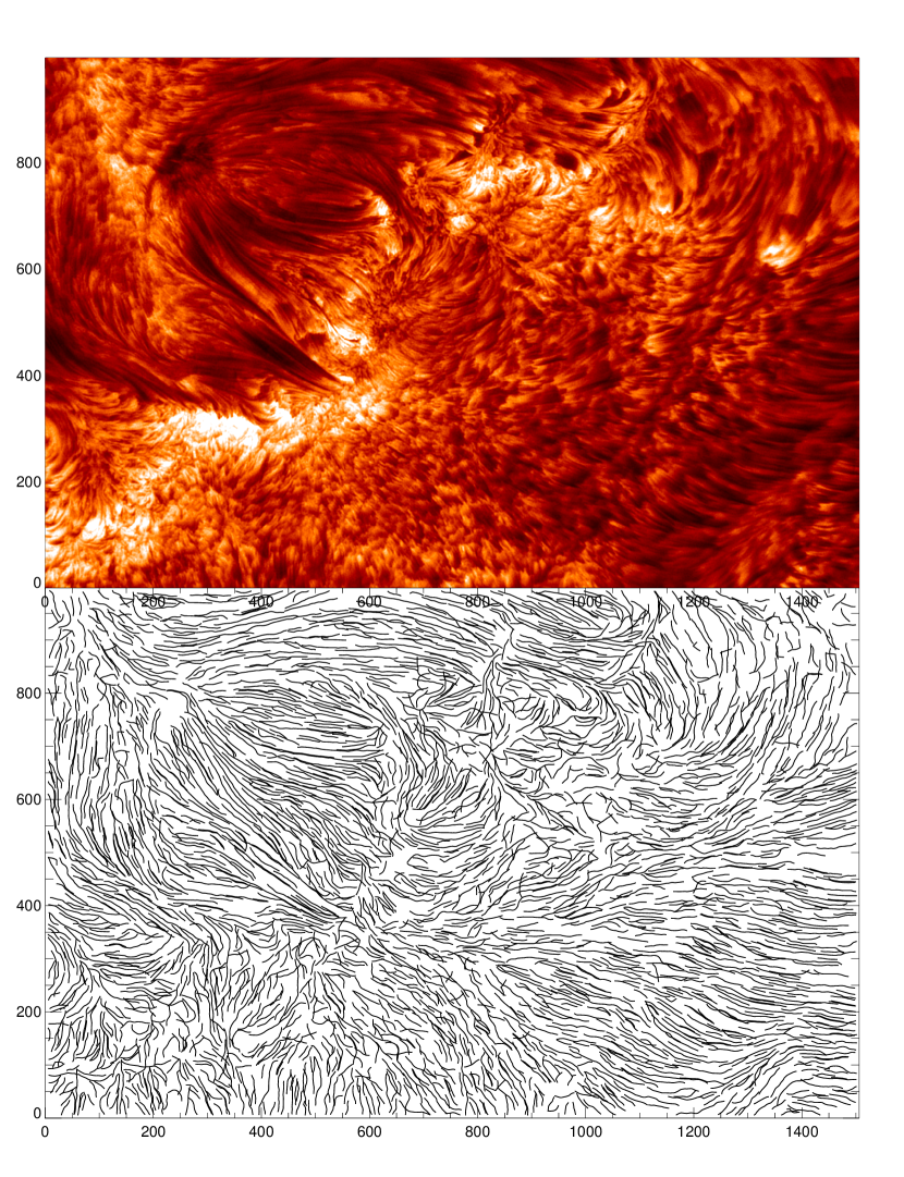
Figure 5: High-resolution image of the solar Active Region 10380, recorded on 2003 June 16 with the Swedish 1-m Solar Telescope (SST) on La Palma Spain (top panel) and automated tracing of curvi-linear structures with a lowpass filter of $n_{sm1}=3$ pixels, a highpass filter of $n_{sm2}=5$ pixels, and a minimum curvature radius of $r_{min}=30$ pixels, tracing out 1757 curvi-linear segments (bottom panel).

3.3 SST Data

Now we apply automated loop tracing to a solar image in a completely different wavelength, namely in the H$\alpha$ 6563 Å line, the first line of the Balmer series of hydrogen. Fig. 5 shows such an image of the solar upper chromosphere, which displays chromospheric spciules in the right side of the picture and filamentary structures in the upper chromosphere and transition region (in altitudes $\approx 2000-5000$ km above the solar surface) depontieu2004 ; depontieu2006 . The image was taken with the Swedish 1-m Solar Telescope (SST) on La Palma, Spain, using a tunable filter, tuned to the blue-shifted line wing of the H$\alpha$ 6563 Å line. The spicules are jets of moving gas at a lower temperature than the million degree hot corona and flow upward from the chromosphere to the transition region with a speed of $\approx 15$ km s^-1 depontieu2004 . The image has a size of $1507\times 999$ pixels ($62\times 41$ Mm on the solar surface), with a pixel size of $0.041\hbox{${}^{\prime\prime}$}$ (or 30 km on the solar surface). This picture is particularly intriguing for automated tracing of curvi-linear structures because of the ubiquity and complexity of fine structure.

This SST image has such a high contrast so that there is no significant noise that affects curvi-linear tracing. Thus, we set the background level to zero ($q_{med}=0.0$) in the OCCULT-2 code. We vary the lowpass filter constant in the range of $n_{sm1}=1,...,21$, set the highpass filter constant to $n_{sm2}=n_{sm1}+2$, and vary the minimum curvature radius in the range of $r_{min}=10,...,100$ pixels. We find a maximum number of detected structures of $N_{det}(L>70)=376$ (with a length above 70 pixels) at $n_{sm1}=3$ and $N_{sm2}=5$ (Fig. 3, middle row left panel), and $r_{min}=40$ pixels (Fig. 3, middle row right panel). Extending to shorter segments with lengths of $L>30$ pixels, the automated tracing code identifies a total of 1757 curvi-linear segments, which outline the patterns of the flow field in the upper chromosphere (Fig. 5, bottom panel).

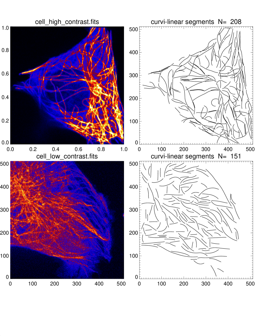
Figure 6: False-coloured images of microtubule filaments in live cells: a high-contrast image of CHO cell (top left panel, Cell-HC), a low-contrast image of U2OS cell (bottom left panel; Cell-LC). The size of the images corresponds to 34 $\mu$m. The automated curvi-linear tracing of both images was carried out with the parameters: $n_{sm1}=3$, $n_{sm2}=5$, and $r_{min}=15$ for Cell-HC, and $n_{sm1}=7$, $n_{sm2}=9$, and $r_{min}=30$ for Cell-LC.

4 Applications to Biophysics

Finally we apply our automated tracing code to images obtained in cellular biophysics, in order to test the versatility and universality of the OCCULT-2 code. As an example, we chose microscopy images of microtubules, but the same approach could be applied to any other filament-like structures: intermediate or actin filaments, fibrin, etc. Microtubules are long stiff polymers that are part of cytoskeleton (internal cellular scaffolding). They are important for cell division, motility and organization (kaverina2011 , deforges2012 ). The entangled network of microtubules serves as a “railroad” system for delivery of cargos by molecular motors and also as a stiff carcass controlling cellular mechanics (deforges2012 , subramanian2012 ). It is a dynamic network adapting and changing in time in response to external cues. The automated extraction of the microtubules network’s configuration from microscopy images and movies can provide insights on the mechanisms of these changes.

Fig. 6 shows two images of cells from two different cell lines with microtubules networks of different density. Cells belonging to CHO cell line (Fig. 6 top, image Cell-HC) are small and have sparse microtubule network. Cells from U2OS line (Fig. 6 bottom, image Cell-LC) are larger and contain more dense radial network. Since microtubules are transparent to the visible light, a fluorescent tag is used to observe them in the living cells. In the analyzed images (Fig. 6) microtubules were labeled with a green fluorescent protein (GFP) (tsien1998 ) that adsorbs light at 490 nm and has an emission peak at 510 nm wavelength. The images were acquired with a spinning disk confocal microscope using the corresponding GFP’s emission filter. The magnified image was projected on the 16-bit chip of camera with dimensions of $512\times 512$ pixels resulting in the final image pixel size of 66 nm. The width of microtubules filaments measured in the electron microscopy studies is about 25 nm (wade1993 ). Due to the diffraction limit the effective width of microtubules in the image is much larger and is defined by the microscopy setup and the wavelength used (abbe1884 ). In our case it is approximately equal to a half of the emission wavelength (510 nm) that is close to the measured microtubule width of $4.7\pm 2.0$ pixels. The two pictures shown in Fig. 6 (left) show cases of opposite contrast, one with high contrast (Fig. 6 top, image Cell-HC), and one with low contrast (Fig. 6 bottom, image Cell-LC). The difference in contrast is explained by a different amount of GFP fluorescent tag associated with microtubules. The automated tracing of the cell filaments provides their locations inside cell and curvature radii, from which flexural rigidity and mechanical stress can be inferred.

We optimize the automated filament tracing by varying the bipass filter constants and find a maximum number of detected filaments (with lengths $L>70$ pixels) with $n_{sm1}=3$, $n_{sm2}=5$, $r_{min}=50$ for the high-contrast cell image, and $n_{sm1}=7$, $n_{sm2}=9$, $r_{min}=40$ for the low-contrast cell image (Fig. 3). The low-contrast image has a higher degree of noise, and thus the filter constants have to be adjusted to a larger value for the low-contrast cell image ($n_{sm1}=7$) than for the high-contrast image ($n_{sm1}=3$).

5 Discussion and Conclusions

5.1 Optimization of Automated Curvi-Linear Tracing

The efficiency and accuracy of automated curvi-linear tracing can be controlled by a number of tuning or control parameters. For the present OCCULT-2 code we have three independent control parameters ($n_{sm1},r_{min},q_{med}$). A prerequisite for the application of curvi-linear tracing codes is the assumption that the structures of interest have a much smaller width $w$ than their length $l$, so that they can be represented by a 1D path, which is generally curved, possibly limited by a minimum curvature radius $r_{min}$. The larger the minimum curvature radius is, the less ambiguity there is for tracing of crossing 1D structures. In this study we explored the parameter space of the control parameters $n_{sm1}$ and $r_{min}$ in order to optimize the performance of the automated tracing code.

The lowpass filter ($n_{sm1}$) and highpass filter ($n_{sm2}$) represent the brackets or scale range of a bandpass filter, bracketing the range of cross-sections of detected structures. We expect to find structures with the smallest width preferentially in images with a high signal-to-noise ratio, while noisy images require more smoothing to enhance fine structure, and thus tend to have larger widths due to the smearing effect of the smoothing. We found the narrowest structures indeed in the two images with the highest contrast (i.e., the SST and Cell-HC image), where highpass filters with boxcars of $n_{sm2}=5$ pixels were used. In images with lower contrast, optimum performance occurred for highpass filters of $n_{sm1}=7,...,11$ pixels. In addition, we found that the smallest bandpass filters produce the sharpest structures and thus the highest detection rate of structures. Since a symmetric boxcar requires odd numbers $n_{sm}=1,3,5,...$, the smallest difference between a lowpass and a highpass filter is 2, and thus the optimum combination is expected to be $n_{sm2}=n_{sm1}+2$, which we indeed confirmed also experimentlly.

For the minimum curvature radius we found optimum performance for a typical range of $r_{min}\approx 30,..,50$ pixels (Fig. 3), which seems not to depend on the contrast of the image.

The control parameter $q_{med}=1$ suppresses faint structures in an image that are below the median value of the image brightness. A meaningful value for this parameter depends very much what fraction of the image contains bright structures of interest, which has to be decided depending on the area ratio of structures of interest to non-relevant background area. If the background has comparable brightness to the structures of interest, a thresholded separation may be impossible, but may still succeed if the background has a different texture than the curvi-linear features (see examples in Fig. 1, where moss and transition region emission have a different texture than coronal loops, while background ripples have the same texture as straight loops and can only be separated by a threshold control parameter). Future efforts aim to synthesize the loop tracings from multi-wavelength image sets, which are more robust and representative for magnetic modeling than single-wavelength images (aschwanden2013b ).

In conclusion, we recommend the following procedure to achieve optimum performance of the curvi-linear tracing code (OCCULT-2): (1) Start with the following recommended control settings: $n_{sm1}=1$, $n_{sm2}=3$, $r_{min}=30$, and $q_{med}=1.0$; (2) Vary the filter combination in the range of $n_{sm1}=1,3,...,15$, while setting $n_{sm2}=n{sm1}+2$, to find the maximum detection rate for a given loop length (e.g., here we used $L>70$ pixels); (3) Low-contrast images are likely to require higher highpass filter values $n_{sm2}$ than high-contrast images. (4) Vary the minimum curvature radius $r_{min}$ within some range to find the maximum detection rate of structures; (5) If the code yields a lot of random structures in obvious background areas, increase the base level factor $q_{med}>1$.

The software of the numerical code OCCULT-2 is publicly accessible in the Interactive Data Language (IDL) in the Solar Software (SSW) package. A tutorial and example is accessible at the authors homepage http://lmsal.com/$\sim$aschwand/software/.

5.2 Solar Applications

The automated tracing of curvi-linear structures in solar physics has mostly been applied to extreme-ultraviolet or soft X-ray images, which show magnetized coronal loops that outline the coronal magnetic field, due to the low plasma-$\beta$ parameter in the solar corona (which is defined as the ratio of the thermal to the magnetic pressure). Thus, coronal loops represent the perfect tracers of the otherwise invisible coronal magnetic field. Standard magnetic field models of the solar corona or parts of it, such as sunspot regions and active regions, have been modeled by extrapolating a photospheric magnetogram, either with a potential field solution or a force-free solution of Maxwell’s equations. However, since the chromosphere was found not to satisfy the force-free condition metcalf1995 , extrapolations of photospheric magnetograms do not exactly render the coronal magnetic field, while coronal loops outline the true coronal magnetic field. It is therefore desirable to trace such coronal loops in EUV and soft X-ray images and to use them to constrain a magnetic field solution. Such attempts have been performed with single EUV images as well as with stereoscopic EUV image pairs aschwanden2013a . Forward-fitting of theoretical magnetic field models to traced coronal loops is able to discriminate between potential field and force-free field models, as well as to quantify the free magnetic energy (that is released in solar flares) and Lorentz forces, e.g., gary2009 . Curvi-linear tracing of filamentary structures in the chromosphere and transition region (Fig. 5) may also help to constrain the horizontal magnetic field components in the non-forcefree regions, which has been used in pre-processing of solar force-free magnetic field extrapolations fuhrmann2011 .

One fundamental limitation of automated coronal loop tracing is the confusion by background structures resulting from EUV emission from the transition region, which has generally a cooler temperature than the coronal loops. Future efforts may use multi-wavelength image data sets to discriminate EUV emission from the chromosphere, transition region, and the corona by its temperature, using a a deconvolution of the multi-wavelength temperature filter response functions in terms of a differential emission measure (DEM) method.

5.3 Biological Applications

The method of curvi-linear tracing is increasingly used in the analysis of biological and medical images, such as to characterize blood vessel tracking in retinal images jiang2007 ; tang2004 ; martinez1999 , neurons xiong2006 , dendritic spines zhang2007 , or microtubule tracing in fluorescent and phase-contrast microscopy brangwynne2007 ; sargin2007 ; koulgi2010 , as shown in Fig. 6. In our experiment with a high-contrast (Fig. 6, top panel) and low-contrast image (Fig. 6, bottom panel), we demonstrated that a bipass or bandpass filter with a bandpass factor of $n_{sm2}=n_{sm1}+2$ enhances the structures to an optimum contrast for automated tracing. Moreover we found that the bandpass filter of low-contrast images requires a larger width ($n_{sm2}=9$ pixels in Fig. 6, bottom panel) than in a high-contrast image ($n_{sm2}=5$ pixels in Fig. 6, top panel).

In our optimization exercise we concentrated mostly on the completeness of detected long curvi-linear segments, but future efforts may also consider the optimization of linking multiple segments that are interrupted with gaps or subject to crossings. The efficiency and reliability of automated curvi-linear algorithms became more important with the massive increase of imaging data over the last decade, which exceeds our limited capabilities of visual inspection. Note that the algorithm used here tracks curvi-linear structures that differ by 16 orders of magnitude in size, from 66 nm to 360 km (pixel size in images).

6 Appendix A: Analytical Description of the OCCULT-2 Code

The Oriented Coronal CUrved Loop Tracing (OCCULT-2) code version 2 is an improved version of the original OCCULT code described in Aschwanden (2010). The improvements include: (1) a “curved” guiding segment that is adjusted to the local curvature radius of a traced loop (representing the second-order term of a polynomial), rather than the linear (first-order polynomial) guiding segment used in the original version, (2) suppression of faint structures, (3) bypass filtering instead of highpass filtering, and (4) simplification of selectable free parameters.

The input is a simple 2-dimensional (2D) image $z_{ij}$, with pixel numbers $i=0,...,n_{x}-1$ on the x-axis, and $j=0,...,n_{y}-1$ on the y-axis, respectively. The output is a number of curvi-linear structures (also called “loops” for short), which are parameterized in terms of x and y-coordinates, $[x(s_{k}),y(s_{k})]$, where the loop length coordinate $s_{k}=0,...,n_{s}$ is given in steps of $\Delta s=1$ pixel, so that for all $k=0,...,n_{s}-1$,

$$\Delta s_{k}=\sqrt{\left([x(s_{k}-x(s_{k-1})]^{2}+[y(s_{k})-y(s_{k-1})]^{2}\right)}=1,\quad k=0,...,n_{s}-1\ ,$$ (2)

with $n_{s}$ the number of loop points for each loop.

The goal of the algorithm OCCULT-2 is to retrieve as many curvi-linear structures as possible, without picking up false signals of non-existing structures in the noise of the image, which has some probability to form chains of random points in a curved array configuration. The challenges are therefore to evaluate an optimum threshold level that separates existing loops from noise structures, and to retrieve the real curvi-linear structures as completely as possible, without subdividing them into partial loop segments. Our strategy to obtain a fast numeric code is to retrieve the loops in a one-dimensional search algorithm, because any two-dimensional concept has a computation time that grows with the square of the image size. The one-dimensional parameter space is essentially the loop length coordinate $s_{k}$, $k=0,...,n_{s}-1$. In addition we define two other independent parameters in each loop point, which can be considered as the first-order and second-order term of a polynomial, namely the local direction angle $\alpha_{l}$, $l=0,...,n_{\alpha}$, and the curvature radius $r_{m}$, $m=0,...,n_{r}$. The algorithm selects iteratively the brightest position $(x_{i},y_{j})$ in the image and starts a bi-directional loop tracing, determining first the local direction $\alpha_{l}(x_{i},y_{j})$ and curvature radius $r_{m}(x_{i},y_{j})$ at the starting point, and continues tracing the loop within a small (guided) range of the local curvature radius, which is the principle of “orientation-guided tracing”. So we are dealing essentially with 1D-tracing in a 5D-parameter space $(x_{i},y_{j},s_{k},\alpha_{l},r_{m})$, which we parameterize with the 5 indices $(i,j,k,l,m)$ that have the index ranges $i=0,...,n_{x}-1,j=0,...,n_{y}-1,k=0,...,n_{s},l=0,...,n_{\alpha},m=0,...,n_{r}$. Specifically, we define the arrays,

$$s_{k}^{bi}=\Delta s\ (k-{n_{s}\over 2})\ ,\quad k=0,...,n_{s}-1\ ,$$ (3)

for a symmetric bi-directional array, used in the search of the local direction $\alpha_{l}$, and

$$s_{k}^{uni}=\Delta s\ k\ ,\quad k=0,...,n_{s}-1\ ,$$ (4)

for a uni-directional array, used in the search for the curvature radius in the forward-direction of a traced structure. For the directional angle $\alpha_{l}$, which is only determined at the starting point of the loop, we use a fixed array with a resolution of one degree (or $\pi/180$ radian),

$$\alpha_{l}=\pi\left({l\over n_{\alpha}}\right)\ ,\qquad l=0,...,n_{\alpha}\ ,\quad n_{\alpha}=180\ .$$ (5)

For the curvature radii $r_{m}$ we use a reciprocal scaling in order to obtain a uniform distribution of directional angles at the end of a curvature segment,

$$r_{m}={r_{min}\over[-1+2m/(n_{r}-1)]}\ ,\qquad n_{r}=30\ .$$ (6)

This parameterization covers positive and negative curvature radii in the ranges of $[-\infty,-r_{min}]$ and $[r_{min},+\infty]$. The choice of an even number $n_{r}$ prevents the singularity $r_{m}=\pm\infty$.

Now we describe the consecutive steps of the algorithm one by one, which follow more or less the same flow chart as depicted in Figure 1 of Aschwanden (2010).

(1) Image base level $(q_{base}$): If the image consists of high-contrast structures without unwanted secondary structures in the background, we do not have to worry about the image base level and can set it to the lowest value (which should be zero or positive in astrophysical images that record an intensity or brightness). However, if there are unwanted structures at a faint brightness level, we can just set the image base level $z_{base}$ above the brightness level of unwanted structures, which we parameterize with the factor $q_{med}$ in units of the median brightness level $z_{med}=median[z_{i,j}]$,

$$z_{base}=z_{med}\times q_{base}\ ,$$ (7)

so that the corrected brightness $z_{i,j}^{\prime}$ in each pixel fulfills the condition

$$z_{i,j}^{\prime}\geq z_{base}\ .$$ (8)

For $q_{med}=0$ the image is unchanged, while the image $z_{i,j}^{\prime}$ appears to be flat in the fainter half area of the image, if set $q_{med}=1.0$. So, the value $q_{med}$ can be adjusted depending on the estimated fraction of the image that is covered with structures of interest. For solar images, this feature offers a convenient way to filter out coronal loops in active regions (which are bright) from unwanted structures in the Quiet Sun (which are faint).

(2) Bandpass Filtering ($n_{sm1},n_{sm2}$): The tracing of curvi-linear structures is considerably eased by enhancing of fine structures within a chosen bandpass that corresponds to the typical width $n_{w}$ of structures of interest, which is typically a few pixels, and assuming that the curvi-linear structures has a much longer length $n_{s}$ than width, i.e., $n_{s}\gg n_{w}$. We accomplish the enhancement with a bandpass filter, which consists of a lowpass filter with a boxcar $n_{sm1}$ and a highpass filter with a boxcar $n_{sm2}$,

$$z_{i,j}^{filter}=smooth[z_{i,j}^{\prime},n_{sm1}]-smooth[z_{i,j}^{\prime},n_{sm2}]\ ,$$ (9)

which filters out broad structures with widths $n_{w}\lower 1.72218pt\hbox{$\;\buildrel>\over{\scriptstyle\sim}\;$}n_{sm2}$ (highpass filter), but smoothes out fine structure with a boxcar of $n_{sm1}<n_{sm2}$. We experimented with a large number of combinations $(n_{sm1},n_{sm2})$ and found that the optimum choice is,

$$n_{sm2}=n_{sm1}+2\ ,$$ (10)

which follows the principle of maximum possible smoothing of fine structures with a given width $n_{sm2}$. The values for the smoothing with a symmetric boxcar has to be an odd integer, i.e., $n_{sm1}=1,3,5,...)$, which implies $n_{sm2}=3,5,7,...$, where the lowest value $n_{sm1}=1$ corresponds to the original image without any smoothing. This experimentally tested relationship for the optimum choice of bandpass filters $(n_{sm1},n_{sm2})$ reduces also the possible parameter space by one dimension, and thus we have search only for $n_{sm1}=1,3,5,...$, while using $n_{sm2}=n_{sm1}+2$.

(3) Noise Threshold: Our algorithm starts with the brightest curvi-linear structure and proceeds to fainter structures, and thus we have to find a stop criterion that halts the procedure when it reaches the level of data noise. Such a noise threshold has to be determined empirically for every image, since there are many sources of possible data noise. Testing many images with completely different data types, we found that a most reasonable threshold level can be determined by an interactive choice of a noise area in the image that contains typical data noise but little structures of interest. Such an image area can be characterized by the pixel ranges $(i_{n1}:i_{n2},j_{n1}:j_{n2})$. In this noise area we determine the median brightness $z_{med}^{noise}$ and define a noise threshold at the doubled value,

$$z_{thresh}=2\times(z_{med}^{noise}>0)\ ,$$ (11)

using only the pixels with positive values in the noise area (in order to prevent a too low value of $z_{thresh}=0$ in the case when more than 50% of the noisy pixels are below the previously chosen base value $z_{base}$). The rationale for the factor 2 in the threshold level comes from the fact that the median separates out only half of the noisy pixels, while the double value would separate out all noisy pixels if the distribution of noisy pixel values follows a linear relationship.

(4) Start of Curvi-Linear Structures: We are ready now to trace the first curvi-linear structure. We determine the location $(i_{0},j_{0})$ of the absolute brightness maximum $z_{0}$ in the bandpass-filtered image $z_{i,j}^{filter}$,

$$z_{0}=z(x_{0},y_{0})=max[z_{i,j}^{filter}(x_{i},y_{j})]\ .$$ (12)

The rationale for the choice of this starting point is the expectation to trace first the most significant structure in the bandpass-filtered image, which can then be continued by going to the next-significant structure, once the tracing of the first structure has been successfully completed and the corresponding loop area is eliminated in a residual image. Consequently, the maximum of the brightness in the residual image marks the second-brightest structure and we can repeat the same procedure by tracing the next loop.

(5) Loop Direction at Starting Point: The next element of the structure to be traced is the first-order term of a polynomial, the direction angle $\alpha_{l}$, which is also the direction of a possible ridge that outlines the local segment of the structure. We determine this directional angle simply by measuring the flux averaged over a straight loop segment symmetrically placed over the starting point $(i_{0},j_{0})$ and rotated over a full range of possible angles $\alpha_{l}$ from $0^{\circ}$ to $180^{\circ}$ degrees. The x,y-coordinates of this linear segment are, with the array $s_{k}^{bi}$ defined by Eq. (5),

$$x_{k,l}=i_{0}+s_{k}^{bi}\cos{\alpha_{l}}\ ,$$ (13)

$$y_{k,l}=j_{0}+s_{k}^{bi}\sin{\alpha_{l}}\ ,$$ (14)

where the index $k$ runs along the length $s_{k}$ of the segment, and the index $l$ denotes a particular angle $\alpha_{l}$. Among the set of angular values $\alpha_{l}$ we determine the maximum of the summed flux in each rotated segment,

$$z_{max}(\alpha_{l})=max_{l}{\left[{1\over n_{s}}\sum_{k=0}^{n_{s}-1}z^{filter}(x_{k,l},y_{k,l})\right]}\ ,$$ (15)

which yields the local direction $\alpha_{max}=\alpha_{l}(l=l_{max})$. In the ideal case of a straight ridge with a constant value $z_{0}$ along the ridge segment with length $n_{s}$ pixels and zero-values outside, a value of $z_{\parallel}=z_{0}$ is found, while the value for a segment in perpendicular direction to the ridge is much smaller, namely $z_{\perp}=1/n_{s}$. This ridge criterion works even for a close succession of parallel ridges, in which case it is still a factor of 2 smaller than in parallel direction, i.e., $z_{\perp}=1/2$.

Figure 7: Geometry of curvature radii centers $(xr_{m},yr_{m})$ located on a line at angle $\beta$ (dash-dotted line), perpendicular to the tangent at angle $\alpha$ (solid line) that intersects a curvi-linear feature (thick solid curve) at position $(x_{0},y_{0})$. The angle $\gamma$ indicates the half angular range of the curved guiding segment (thick solid line).

(6) Local curvature radius: Next we determine the second-order term of a polynomial that follows the loop to be traced. We define a directional angle $\beta_{0}$ that is in perpendicular direction to the loop and defines the direction where all centers of possible curvature radii are located (that intersect the structure at location $(x_{0},y_{0})$), see geometric definition of the angles $\alpha$ and $\beta$ in Fig. 7,

$$\beta_{0}=\alpha_{0}+{\pi\over 2}\ .$$ (16)

The location $(x_{c},y_{c})$ of the curvature center with a minimum curvature radius $r_{min}$ is then found at,

$$x_{c}=x_{0}+r_{min}\cos{\beta_{0}}\ ,$$ (17)

$$y_{c}=y_{c}+r_{min}\sin{\beta_{0}}\ .$$ (18)

The loci of all curvature centers $(x_{m},y_{m})$ of a set of curvature radii $r_{m}=r_{min}/[-1+2m/(n_{r}-1)]$ (Eq. 6) is then found at,

$$x_{m}=x_{0}+(x_{c}-x_{0}){r_{m}\over r_{min}}\ ,$$ (19)

$$y_{m}=y_{0}+(y_{c}-y_{0}){r_{m}\over r_{min}}\ .$$ (20)

Since we want to follow a loop along a curved segment for every possible curvature radius $r_{m}$, we determine the coordinates for each segment point $s_{k}$. It is useful to define the angle $\beta_{m}$ of the line that connects a curvature center $(x_{m},y_{m})$ with a curved segment point $s_{k}$,

$$\beta_{m}=\beta_{0}+\sigma_{dir}\left({s_{k}\over r_{m}}\right)\ ,$$ (21)

where $\sigma_{dir}=\pm 1$ has two opposite signs, depending on the forward or backward tracing of a loop. The x,y-coordinates $(x_{km},y_{km})$ of the loop segment $s_{k}$ is then,

$$x_{km}=x_{m}-r_{m}\cos{(\beta_{m})}\ ,$$ (22)

$$y_{km}=y_{m}-r_{m}\sin{(\beta_{m})}\ .$$ (23)

In order to determine the curvature radius $r_{m}$ that fits the local loop segment best, we search for the segment with the maximum flux along the curve with radius $r_{m}$,

$$z_{max}=max_{m}[{1\over n_{r}}\sum_{k=0}^{n_{s}-1}z_{i,j}^{\prime}(x_{km},y_{km})]\ .$$ (24)

Since we know now the optimum curvature radius $r_{m}$, we can trace the loop incrementally by a step $\Delta s$ and extrapolate the position $(x_{k+1},y_{k+1})$ and angle $\alpha_{k+1}$ by

$$\alpha_{k+1}=\alpha_{k}+\sigma_{dir}{\Delta s\over r_{m}}\ ,$$ (25)

$$\alpha_{mid}={(\alpha_{k}+\alpha_{k+1})\over 2}\ ,$$ (26)

$$x_{k+1}=x_{k}+\Delta s\cos{\left[\alpha_{mid}+(\pi/2)(1+\sigma_{dir})\right]}\ ,$$ (27)

$$y_{k+1}=y_{k}+\Delta s\sin{\left[\alpha_{mid}+(\pi/2)(1+\sigma_{dir})\right]}\ .$$ (28)

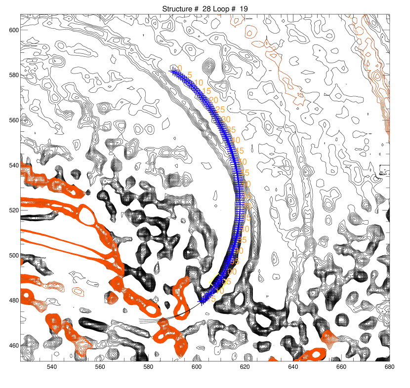
Figure 8: Example of loop tracing in the pixel area [525:680, 453:607] of the image shown in Fig. 2. Loop #19 is traced (blue crosses) over a length of 115 pixels (orange numbers), crossing another structure at a small angle. The curves at position 115 indicate the three curved segments that have been used in the tracing of the last loop point. The black contours indicate the bandpass-fitlered difference image, and the red contours indicate the previously traced and erased structures in the residual difference image.

(7) Bidirectional tracing: The step (6) describes the extrapolation or tracing of the loop segment from position $s_{k}=(x_{k},y_{k})$ to $s_{k+1}(x_{k+1},y_{k+1})$ by an incremental length step $\Delta s$. This step is repeated, starting from some arbitrary starting point $s_{0}$ inside the segment until the first endpoint $s_{n_{s1}}$, where the traced curvi-linear structure seems to end. The first endpoint generally is demarcated at a location where the bandpass-filtered image has zero or negative values, so one could just detect the first image pixel along the guiding segment $s_{k}$ that is non-positive. However, in order to allow for some minor gaps in noisy structures, it turned out to be more reliable to define a stop criterion when a least a few pixels have a nonpositive value, say $n_{gap}=3$ pixels. An example of a traced loop is shown in Fig. 8, which illustrates that a loop can reliably be traced even in the presence of secondary loops that intersect at small angles.

After completing the first half segment ($\sigma_{dir}=+1$), we repeat the same procedure from the midpoint $(x_{0},y_{0})$ in opposite direction ($\sigma_{dir}=-1$), until we stop at the second endpoint at $s_{n_{s2}}$. We combine than the two segments $[s_{0},s_{n1}]$ and $[s_{0},s_{n2}]$ by reversing one segment in order to maintain the same direction, and concatenating the two equal-directed segments into a single loop structure with indices $[s_{0},...,s_{n_{s}}]$, where the length is $s_{n}=(s_{n_{1}}+s_{n2})$.

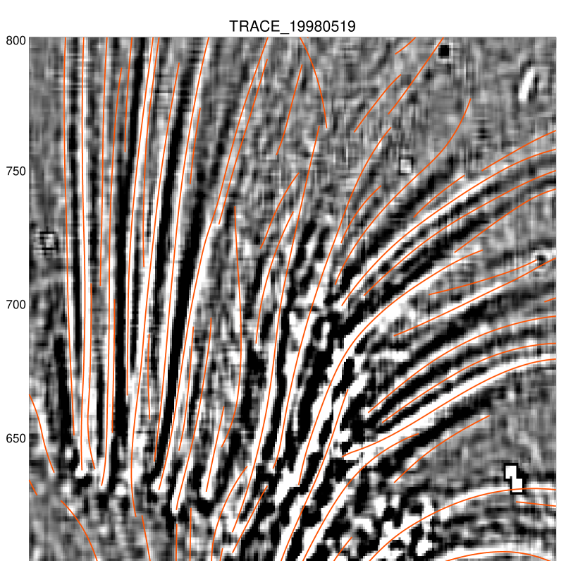
Figure 9: Example of loop tracings in area [300:550, 600:800] of the full image shown in Fig. 2. The greyscale indicates the bandpass-filtered image $(n_{sm1}=5,n_{sm2}=7)$, and the loop tracings are shown with red curves.

(8) Loop Iteration: The steps (4) to (7) describe the tracing of a single loop, specified by the $n_{L}$ coordinates $(x_{i},y_{i})=[x(s_{k}),y(s_{k})],k=0,...,n_{L}-1$. In order to proceed to the next loop we want first to erase the area of this traced loop in the residual image, so that no previously traced loop segment is traced a second time in a consecutive loop. The loop is erased in the residual image simply by setting those image pixels to zero that have a distance of $d\leq n_{w}=(n_{sm2}/2-1)$ from the loop coordinates, i.e., $z^{filter}[x_{i}\pm n_{w},y_{j}\pm n_{w}]=0$. An example of an image area with dense coverage of loops is shown in Fig. 9, where some loops are traced at flux levels close to the noise threshold.

(9) Loop Parameters: After we described analytically the numerical code, we summarize the free parameters and the dependent parameters (that do not require any selection by the user of the code). The code has the following free or input parameters: the lowpass filter boxcar $n_{sm1}$, the minimum curvature radius $r_{min}$, the base level factor $q_{med}$, in units of image median brightness values, and the corner coordinates of the noise area $[i_{n1}:i_{n2},j_{n1}:j_{n2}]$. All other parameters are dependent, or a fixed constant, such as the tracing step $\Delta s=1$, the highpass filter boxcar $n_{sm2}=n_{sm1}+2$, the half width of the erased loop cross-sections $n_{w}=n_{nsm2}/2-1$, and the loop termination gap $n_{gap}=3$.

- (1) Abbe, E. Note on the proper definition of the amplifying power of a lens or a lens-system, J. Royal Microsc. Soc. 1884, 4, 348-351.
- (2) Aschwanden, M.J. and Nightingale, R.W. Elementary loop structures in the solar corona analyzed from TRACE triple-filter images. Astrophys. J. 2005, 633, 499-517.
- (3) Aschwanden, M.J., Lee, J.K., Gary, G.A., Smith, M., and Inhester, B. Comparison of Five Numerical Codes for Automated Tracing of Coronal Loops. Solar Phys. 2008, 248, 359-377.
- (4) Aschwanden, M.J. A Code for Automated Tracing of Coronal loops Approaching Visual Perception. Solar Phys. 2010, 262, 399-423.
- (5) Aschwanden, M.J. Nonlinear Force-free Magnetic Field Fitting to Coronal Loops with and without Stereoscopy, Astrophys. J. 2013, 763, 115.
- (6) Aschwanden, M.J. and Sun. Y. The Active Region 11158 during the 2011 February 15 X-Class Flare: Nonlinear Force-free Magnetic Fields and Free Energies Inferred from Automated Loop Tracing, (in preparation).
- (7) Biskri, S., Antoine, J.-P., Inhester, B., and Mekideche, F. Extraction of Solar Coronal Magnetic Loops with the Directional 2D Morlet Wavelet Transform, Solar Phys., 2010, 262, 373.
- (8) Brangwynne, C.P., Koenderingk, G.H, Barry, E., Dogic, Z., MacKintosh, F.C., and Weitz, D.A. Bending dynamics of fluctuating biopolymers probed by automated high-resolution filament tracking, Biphys. J., 2007, 93/(1), 346-359.
- (9) de Forges, H., Bouissou, A., Perez, F. Interplay between microtubule dynamics and intracellular organization, Int. J. Biochem Cell Biol. 2012, 44, 266-274.
- (10) De Pontieu, B., Erdelyi, R., and James, S.P. Solar chromospheric spicules from the leakage of photospheric oscillations and flows, Nature 2004, 430, 536-539.
- (11) De Pontieu, B., Carlsson, M., Rouppe van der Voort, L., Löfdahl, M., van Noort M., Nordlund, Å., and Scharmer, G. Rapid temporal variability of faculae: high-resolution observations and modeling, Astrophys. J., 2006, 1405-1420.
- (12) Fuhrmann, M., Seehafer, N., Valori, G., and Wiegelmann, T. A comparison of preprocessing methods for solar force-free magnetic field extrapolation, Astron. Astrophys. 2011, 526, A70.
- (13) Gary, G.A. Evaluation of a selected case of the minimum dissipative rate method for non-force-free solar magnetic field extrapolation, Solar Phys. 2009, 257, 271-286.
- (14) Gonzales, R.C., Woods, R.E.. Digital Image Processing, Pearson Prentice Hall, Upper Saddle River, NJ 07458, 2008, p.689-794.
- (15) Jiang, Y., Bainbridge-Smith, A., and Morris, A.B. Blood vessel tracking in retinal images, in Proc. of Image and Vision Computing New Zealand, December 2007, p.126-131.
- (16) Kaverina, I. and Straube A. Regulation of cell migration by dynamic microtubules, Semin. Cell Dev. Biol., 2011, 22, 968-974.
- (17) Koulgi, P., Sargin, M.E., Rose, K., and Manjunath, B.S. Graphical model-based tracing of curvi-linear structures in bio-image sequences, in IEEE International Conference on Pattern Recognition, 2009, 2596-2599.
- (18) Lee, J.K., Newman, T.S., Gary, G.A. Automated Detection of Solar Loops by the Oriented Connectivity Method. In: Proc. 17th Int. Conf. on Pattern Recognition (ICPR), Cambridge, United Kingdom, 2004, 315.
- (19) Lee, J.K., Newman, T.S., Gary, G.A. Oriented connectivity-based method for segmenting solar loops. Pattern Recognition 2006, 39, 246-259.
- (20) Lemen, J.R., Title, A.M., Akin, D.J., Boerner, P.F., Chou, C., Drake, J.F., Duncan, D.W., Edwards, C.G., et al. The Atmospheric Imaging Assembly (AIA) on the Solar Dynamics Observatory (SDO), Solar Phys. 2012, 275, 17-40.
- (21) Martinez-Perez, M.E., Hughes, A.D., Stanton, A.V., Thom, S.A., Barath, A.A., and Parker, K.H. Segmentation of retinal blood bessels based on the second directional derivative and region growing, in International Conference on Image Processing (ICIP 99, 24-28 October 1999, 2, 173-176.
- (22) McAteer, R.T.J., Gallagher, P.T., and Ireland, J. Statistics of Active Region Complexity: A Large-Scale Fractal Dimension Survey, Astrophys. J. 2005, 631, 628-635.
- (23) Metcalf, T.R., Jiao, L., Uitenbroek, H., McClymont, A.N., and Canfield, R.C. Is the solar chromospheric magnetic field force-free? Astrophys. J. 1995, 439, 474-481.
- (24) Pawley, J.B. and Masters B.R. Handbook of Biological Confocal Microscopy, J. Biomedical Optics 2008, 13/2, p. 029902.
- (25) Sargin, M.E., Altinok, A., Rose, K., and Manjunath, B.S. Tracing curvi-linear structures in live cell images, in IEEE International Conference on Image Processing (ICIP 07, 16-19 September 2007, 6, 285-288.
- (26) Subramaniam, R., Kapoor, T.M. Building complexity: insights into self-organized assembly of microtubule-based architectures, Dev. Cell 2012, 22, 874-885.
- (27) Tang, J. and Acton, S.T. Vessel boundary tracking for intravital microscopy via multiscale gradient vector flow snakes, in IEEE International Conference on Acoustics, Speech, and Signal Processing (ICASSP 04, 17-21 May 2004, 51, no. 2, 316-324.
- (28) Tsien, R.Y. The green fluorescent protein, Annu. Rev. Biochem. 1998, 67, 506-544.
- (29) Wade, R.H., Chrétien, D. Cryoelectron microscopy of microtubules. J. Struct. Biol. 1993, 110, 1-27.
- (30) Xiong, G., Zhou, X, Degterev, A., Ji, L., and Wong, S.T. Automated neurite labeling and analysis in fluorescence microscopy images, Cytometry Part A 2006 69A, no. 6, 494-505.
- (31) Zhang, Y., Zhou, X., Witt, R.M., Sabatini, B.L., Adjeroh, D. and Wong, S.T. Dendritic spine detection using curvi-linear structure detector and Ida classifier, NeuroImage 2007 36, no. 2, 346-360.