DCE: A Novel Delay Correlation Measurement for Tomography with Passive Realization

Abstract

Tomography is important for network design and routing optimization. Prior approaches require either precise time synchronization or complex cooperation. Furthermore, active tomography consumes explicit probeing resulting in limited scalability. To address the first issue we propose a novel Delay Correlation Estimation methodology named DCE with no need of synchronization and special cooperation. For the second issue we develop a passive realization mechanism merely using regular data flow without explicit bandwidth consumption. Extensive simulations in OMNeT++ are made to evaluate its accuracy where we show that DCE measured delay correlation is highly identical with the true value. Also from test result we find that mechanism of passive realization is able to achieve both regular data transmission and purpose of tomography with excellent robustness versus different background traffic and package size.

I Introduction

Network tomography [1] studies internal characteristics of Internet using information derived from end nodes. One advantage is that it requires no participation from network elements other than the usual forwarding of packets while traditional traceroute method needs response to ICMP messages facing challenge of anonymous routers [2].

Many literatures choose delay to calculate correlation between end hosts for tomography. However, they require either precise time synchronization or complex cooperation. Moreover, active way consumes quantities of explicit probing bandwidth which results in limited scalability.

In this paper we propose a novel Delay Correlation Estimation approach named DCE with no need of cooperation and synchronization between end nodes. The greatest property is that we only need to measure the packet arriving time at receivers. To further reduce bandwidth consumption a passive mechanism using regular data flow is developed.

We do extensive simulations in OMNeT++ to evaluate its accuracy. Results show that $\sigma_{d_{a},d_{b}}^{2}$ measured by DCE is highly identical with the true value $\sigma_{s}^{2}$ on shared path. By altering background traffic and package size we see that passive mechanism has excellent robustness and is able to achieve regular data transmission as well as purpose of tomography.

I-A Contributions

• We propose DCE to estimate delay correlation. This method needs no special cooperation or synchronization and avoids issues using RTT, making it largely different from prior tomography tools [3] and [4].

• We develop a passive mechanism for realization that is efficient for bandwidth saving.

• Extensive simulations in OMNeT++ demonstrates its accuracy and robustness.

II Related work

Y. Vardi was one of the first to study network tomography [1] that can be implemented in either an active or passive way. Active network tomography [5], [6], [7] needs to explicitly send out probing messages to estimate the end-to-end path characteristics, while passive network tomography [8], [9], [10], [11] infers network topology without sending any explicit probing messages.

Article [3] describes delay tomography which however, needs synchronization and cooperation between sender and receiver. In [4] authors develop Network Radar based on RTT trying to solve these issues. However, two reasons distort the measurement accuracy. One is due to the variable processing delay at destination nodes and the other is its violation of a significant assumption that return paths of packet are uncorrelated while actually they overlaps.

In addition, delay correlation can be further used for topology recovery [12], [13] that is important to improve network performance.

III DCE for Delay Correlation Measurement

Figure 1: The tree structure: a sender $f$ and two receivers $a$, $b$

A simple model we use in this paper is shown in Fig.1. The routing structure from the sender $f$ to the receivers $a$ and $b$ must be a tree rooted at $f$. Otherwise, there is routing loop which must be corrected. Assume that router $s$ is the ancestor node of both $a$ and $b$. Assume that the sender uses unicast to send messages to receivers, and assume that packets are sent in a back-to-back pair. For the k-th pair of back-to-back packets, denoted as $a^{k}$ and $b^{k}$, sent from $f$ to $a$ and $b$, respectively, we use the following notation:

• $t_{a}(k)$: the time when $a$ receives $a^{k}$ in the k-th pair.

• $t_{b}(k)$: the time when $b$ receives $b^{k}$ in the k-th pair.

• $d_{a}(k)$: the latency of $a^{k}$ along the path from $f$ to $a$.

• $d_{b}(k)$: the latency of $b^{k}$ along the path from $f$ to $b$.

• $t_{f}(k)$: the time when $f$ sends the k-th pair of packets.

Using network model of Fig.1 we obtain Eq.(1) for $a^{0}$ (we start the index with 0 for convenience):

$$t_{a}(0)=t_{f}(0)+d_{a}(0)$$ (1)

Similarly, for $a^{k}$ we have

$$t_{a}(k)=t_{f}(k)+d_{a}(k)$$ (2)

Let Eq.(2) $-$ Eq.(1) and $\delta_{a}(k)\equiv t_{a}(k)-t_{a}(0)$, we can obtain Eq.(3):

$$\delta_{a}(k)=(t_{f}(k)-t_{f}(0))+(d_{a}(k)-d_{a}(0))$$ (3)

Denote the time interval between two consecutive pairs of packets as $\delta$. We assume that $\delta$ is a constant for simplicity at this moment, and relax this assumption later. In this case we use $k\delta\equiv k\cdot\delta$ to replace $t_{f}(k)-t_{f}(0)$ in Eq.(3), then we have

$$d_{a}(k)=\delta_{a}(k)-k\delta+d_{a}(0)$$ (4)

Let $\delta^{\prime}_{a}(k)\equiv\delta_{a}(k)-k\delta$, Eq.(4) is transformed into Eq. (5):

$$d_{a}(k)=\delta^{\prime}_{a}(k)+d_{a}(0)$$ (5)

We can achieve similar result at receiver $b$ as in Eq.(6):

$$d_{b}(k)=\delta^{\prime}_{b}(k)+d_{b}(0)$$ (6)

Where $\delta^{\prime}_{b}(k)\equiv\delta_{b}(k)-k\delta$.

To estimate the correlation between $d_{a}(k)$ and $d_{b}(k)$, we introduce the following lemma.

Lemma 1.

Assuming that $\zeta$, $\eta$ are two random variables, and $\chi=a\zeta+b$, $\gamma=c\eta+d$, where a,b,c,d are constant and a,c have the same symbol, thus we have $\sigma_{\zeta,\eta}^{2}=\sigma_{\chi,\gamma}^{2}$.

Proof:

$$\begin{split}\sigma_{\chi,\gamma}^{2}&=\frac{E(\chi-E\chi)(\gamma-E\gamma)}{\sqrt{D\chi}\sqrt{D\gamma}}\\ &=\frac{E(a\zeta+b-aE\zeta-b)(c\eta+d-cE\eta-d)}{\sqrt{a^{2}D\zeta}\sqrt{c^{2}D\eta}}\\ &=\frac{acE(\zeta-E\zeta)(\eta-E\eta)}{|a||c|\sqrt{D\zeta}\sqrt{D\eta}}\\ &=\frac{E(\zeta-E\zeta)(\eta-E\eta)}{\sqrt{D\zeta}\sqrt{D\eta}}\\ &=\sigma_{\zeta,\eta}^{2}\end{split}$$ (7)

∎

Based on Lemma 1, we have the following theorem:

Theorem 1.

The correlation between delay variables $d_{a}(k)$ and $d_{b}(k)$ is equivalent to the correlation between variables $\delta^{\prime}_{a}(k)$ and $\delta^{\prime}_{b}(k)$, which means

$$\sigma_{d_{a}(k),d_{b}(k)}^{2}=\sigma_{\delta^{\prime}_{a}(k),\delta^{\prime}_{b}(k)}^{2}$$ (8)

Based on the measurements of $\delta^{\prime}_{a}(k)$, $\delta^{\prime}_{b}(k)$ we can calculate the correlation of delays along the path from $f$ to $a$ ($path_{a}$) and long the path from $f$ to $b$ ($path_{b}$), denoted as $\hat{\sigma}_{\delta^{\prime}_{a},\delta^{\prime}_{b}}^{2}$ using Eq.(9):

$$\hat{\sigma}_{\delta^{\prime}_{a},\delta^{\prime}_{b}}^{2}=\frac{1}{n-1}\sum_{k=1}^{n}[\delta^{\prime}_{a}(k)-\overline{\delta^{\prime}_{a}}][\delta^{\prime}_{b}(k)-\overline{\delta^{\prime}_{b}}]$$ (9)

Where $\overline{\delta^{\prime}_{i}}$ is the sample mean of ${\delta^{\prime}_{i}(k)}_{k=1}^{n}$ for $i=a,b$.

Theorem 2.

$\hat{\sigma}_{\delta^{\prime}_{a},\delta^{\prime}_{b}}^{2}$ in Eq.(9) is an unbiased estimator of the correlation on shared path.

Proof:

First of all we show that $\hat{\sigma}_{d_{a},d_{b}}^{2}$ (not $\hat{\sigma}_{\delta^{\prime}_{a},\delta^{\prime}_{b}}^{2}$) is an unbiased estimator of the correlation on shared path $(f,s)$. Let $\lambda_{a}$, $\lambda_{b}$ denote the mean time latency of $path_{a}$, $path_{b}$ and let $\overline{d_{a}}$, $\overline{d_{b}}$ denote the sample mean correspondingly; true correlation ${\sigma}_{d_{a},d_{b}}^{2}=E[(d_{a}(k)-\lambda_{a})(d_{b}(k)-\lambda_{b})]$. To prove that $E[\hat{\sigma}_{d_{a},d_{b}}^{2}]=\sigma_{d_{a},d_{b}}^{2}$ we analyze the expectation of $E[(d_{a}(k)-\overline{d_{a}})(d_{b}(k)-\overline{d_{b}}]$:

$$\begin{split}&E[(d_{a}(k)-\overline{d_{a}})(d_{b}(k)-\overline{d_{b}}]\\ &=E[d_{a}(k)d_{b}(k)]-\frac{1}{n}\sum_{i=1}^{n}E[d_{a}(k)d_{b}(i)]\\ &-\frac{1}{n}\sum_{i=1}^{n}E[d_{a}(i)d_{b}(k)]+\frac{1}{n^{2}}\sum_{i=1}^{n}\sum_{j=1}^{n}E[d_{a}(i)d_{b}(j)]\end{split}$$ (10)

Since delays of the $i^{th}$ and $k^{th}$ pair are independent and

$$\begin{split}{\sigma}_{d_{a},d_{b}}^{2}&=E[(d_{a}(k)-\lambda_{a})(d_{b}(k)-\lambda_{b})]\\ &=E[d_{a}(k)d_{b}(k)]-\lambda_{a}\lambda_{b}\end{split}$$

We obtain Eq.(11)

$$\begin{split}E[d_{a}(k)d_{b}(i)]=\left\{\begin{aligned} &\lambda_{a}\lambda_{b}&k\neq i\\ &\lambda_{a}\lambda_{b}+\sigma_{d_{a},d_{b}}^{2}&k=i\\ \end{aligned}\right.\end{split}$$ (11)

Substituting Eq.(11) into Eq.(10) we obtain

$$\begin{split}E[(d_{a}(k)-\overline{d_{a}})(d_{b}(k)-\overline{d_{b}}]=(\frac{n-1}{n})\sigma_{d_{a},d_{b}}^{2}\end{split}$$

Therefore, $\hat{\sigma}_{d_{a},d_{b}}^{2}$ is an unbiased estimator of the correlation on shared path as is shown in Eq.(12)

$$\begin{split}E[\hat{\sigma}_{d_{a},d_{b}}^{2}]&=\frac{1}{n-1}\sum_{k=1}^{n}E[(d_{a}(k)-\overline{d_{a}})(d_{b}(k)-\overline{d_{b}})]\\ &=\frac{1}{n-1}n(\frac{n-1}{n})\sigma_{d_{a},d_{b}}^{2}=\sigma_{d_{a},d_{b}}^{2}\end{split}$$ (12)

According to $\sigma_{d_{a},d_{b}}^{2}=\sigma_{\delta^{\prime}_{a},\delta^{\prime}_{b}}^{2}$ in Theorem 1 we prove it. ∎

III-A Discussion of $\delta$

III-A1 $\delta$ is a constant

A complete delay correlation estimation algorithm (DCE) is summarized in Algorithm 1 if the time interval $\delta$ is a constant.

Algorithm 1 Delay Correlation Estimation Algorithm

0:    Given time interval $\delta$.

0:    

1:  for $k=0:n$ do

2:     Using Eq.(1) to Eq.(3) to measure $\delta_{a}(k)$ in the $k^{th}$ transmission;

3:     Using $\delta^{\prime}_{a}(k)\equiv\delta_{a}(k)-k\delta$ to calculate $\delta^{\prime}_{a}(k)$;

4:     Similarly measuring $\delta_{b}(k)$ and calculating $\delta^{\prime}_{b}(k)\equiv\delta_{b}(k)-k\delta$;

5:  end for

6:  For all the $\delta^{\prime}_{a}(k)$ and $\delta^{\prime}_{b}(k)$ using Eq.(9) to obtain the unbiased estimator for correlation $\sigma_{\delta^{\prime}_{a},\delta^{\prime}_{b}}^{2}$, which is equivalent to $\sigma_{d_{a},d_{b}}^{2}$ between a, b according to Theorem 1.

III-A2 $\delta$ is not a constant

If the time interval $\delta$ is not a constant then $t_{f}(k)-t_{f}(0)\neq k\delta$. In this case using $k\delta$ to replace $t_{f}(k)-t_{f}(0)$ is inappropriate and we choose $\delta_{f}(k)$ to denote $t_{f}(k)-t_{f}(0)$ in Eq.(3), then Eq.(4) can be rewritten to Eq.(13).

$$d_{a}(k)=\delta_{a}(k)-\delta_{f}(k)+d_{a}(0).$$ (13)

Correspondingly, Eq.(5) and Eq.(6) can be replaced with $\delta^{\prime}_{a}(k)\equiv\delta_{a}(k)-\delta_{f}(k)$ and $\delta^{\prime}_{b}(k)\equiv\delta_{b}(k)-\delta_{f}(k)$, respectively.

Note that $t_{f}(k)$ is a timestamp contained in the packet, and thus $\delta_{f}(k)=t_{f}(k)-t_{f}(0)$ is readily available.

III-B A mechanism for passive realization

To reduce explicit probing we propose a mechanism for passive realization of Algorithm 1 in real networks.

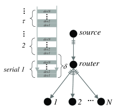
Figure 2: The mechanism for passive tomography with source and N end hosts.

As Fig.2 shows passive realization works as follows. In practical networks (for example, P2P networks) if N end hosts request common contents from a source, it will distribute packets. In this situation source first chooses the No.1 requested data block which is duplicated into packet serial 1 and sent out to all N hosts simultaneously guaranteeing that there exist two successive packets in a back-to-back manner. An indicator (IR) is needed to tell if the received packet at each host belongs to the back-to-back pair. If serial of No.1 is sent completely source repeats to the next until all requested contents are received by N hosts. As regular data flow proceeds transmitting we change destination address of the current two successive packets when delay correlation between the corresponding host pair has been measured (if number of packets sent to them with indicator IR reaches $\tau$ where $\tau$ is a tunable threshold).

One may naturally raise two questions: first is which two successive packets in one serial are chosen to add an IR? while the other is how to guarantee that in each transmission the two successive packets are in a back-to-back manner? A simple mechanism can solve both of them. The basic idea is that we divide packets into small size. This can satisfy both the need of back-to-back and regular data transmission. In fact our experiment results show that any two successive packets in a serial distributed to N hosts can be chosen to add IR as long as the time interval $\delta$ is appropriate.

III-C Arrangement of IR

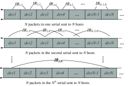
Figure 3: Arrangement of IR. IR_i,j in each serial indicates blocks destined to i, j should be successive.

Based on above argument that each successive pair of packets can be regarded as back-to-back, in one transmitting serial at most N-1 delay correlations are measured (shown in Fig.3). After N-1 times switching of destination addresses and IRs all delay correlations between N hosts can be obtained.

In this way the complexity is only $O(N)$ compared with $O(N^{2})$ to measure $N(N-1)/2$ correlations.

IV Simulation results

IV-A Setups of simulation

Figure 4: Structure for DCE test

We use OMNeT++ for simulations [14] to demonstrate the correctness and robustness of passive DCE tomography. We generate a network shown in Fig.4. Nodes of BG is for producing background traffic while others are the source and client nodes. When two hosts $a$, $b$ request contents from $f$, it will send regular data in a back-to-back manner. In this case route algorithm determines a multicast tree with root $f$ and leaves $a$, $b$.

We set packet hundreds of bytes to satisfy both regular transmission and back-to-back property. One advantage is that since it is smaller than Maximum Transmission Unit (MTU) we avoid delay for package segmentation. We set bandwidth of each link value of 100Mbps; the background traffic pattern conforms to the Poisson distribution, whose expectation value could be set from 1MBps to 12MBps. We also change the size of packet from 100 bytes to MTU to see its influence on DCE measurement.

IV-B Results

Using DCE methodology we set $\tau$ to be 1550 and observe over 1500 timing samples for receiver pair.

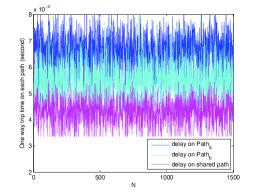
Figure 5: One way trip time latency on $path_{a}$, $path_{b}$ and shared path $(f,s)$

Fig.5 depicts the one way trip latency in our environment. One example of the average delay on $path_{a}$, $path_{b}$ and shared path are 0.6526ms, 0.5478ms and 0.4317ms respectively. In some case errors may happen to the timestamp as the variation of background traffic. Therefore, we ignore packets beyond twice the average delay on each path.

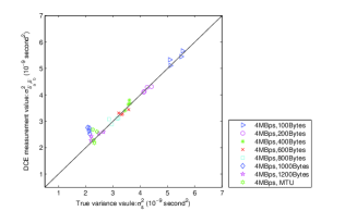
Figure 6: DCE measurement covariance $\sigma_{\delta^{\prime}_{a},\delta^{\prime}_{b}}^{2}$ versus the directly measured delay variance on the shared path $(f,s)$

Fig.6 shows the DCE covariance $\sigma_{\delta^{\prime}_{a},\delta^{\prime}_{b}}^{2}$ versus true value $\sigma_{s}^{2}$ on shared path $(f,s)$. Value $\sigma_{\delta^{\prime}_{a},\delta^{\prime}_{b}}^{2}$ is calculated using the arriving time of package at $a$, $b$ while $\sigma_{s}^{2}$ is calculated directly from delay on $(f,s)$. According to Theorem 1 we know that $\sigma_{d_{a},d_{b}}^{2}$ is equal to $\sigma_{\delta^{\prime}_{a},\delta^{\prime}_{b}}^{2}$ thus, ideally $\sigma_{\delta^{\prime}_{a},\delta^{\prime}_{b}}^{2}$ and $\sigma_{s}^{2}$ should be identical and fall onto the 45 degree line. Taking test result with package size of 800 Bytes for example we see the estimated value is always locating nearby the true value with slight difference which demonstrates the correctness of DCE tomography. If we change size of data packet from 100 bytes to MTU delay correlation measured by DCE is always desired. This demonstrates that passive mechanism is able to achieve both data transmission and tomography.

Figure 7: $\frac{|\sigma_{\delta^{\prime}_{a},\delta^{\prime}_{b}}^{2}-\sigma_{s}^{2}|}{\sigma_{s}^{2}}$: DCE measurement error versus different background traffic

In Fig.7 packet size is fixed to be MTU. In this case performance of DCE tomography is perfect with the percentage error below 4% when the expectation value of background traffic is within the region [1.25MBps,7.5MBps]. However, when it increases to 8MBps, error percentage increases sharply. This is because in this situation network’s performance becomes worse and some shared paths between higher level routers are congested heavily, which destroys the back-to-back property of packets. Note that when the expectation value of background traffic is relatively small (below 1MBps) delay correlation caused by queuing on routers will not be significant thus the performance also degrades.

V Conclusions and future work

In this paper we propose a novel tomography method named DCE to estimate delay correlation with no need of synchronization and cooperation between end hosts. We also develop the passive mechanism to further save bandwidth. Extensive simulations demonstrate the correctness of DCE. Moreover, passive realization is able to achieve both purpose of tomography and data transmission with excellent robustness versus different background traffic and package size.

In future, we plan to utilize the DCE measure for topology tomography.

References

- [1] Y. Vardi, “Network tomography: estimating source-destination traffic intensities from link data,” Journal of the American statistical association, vol. 91, no. 433, pp. 365–377, March 1996.
- [2] B. Yao, R. Viswanathan, F. Chang, and D. Waddington, “Topology inference in the presence of anonymous routers,” in Proceedings of the IEEE INFOCOM, San Francisco, CA, April. 2003, pp. 353–363.
- [3] Y. Tsang and R. D. Nowak, “Network delay tomography,” IEEE TRANSACTIONS ON SIGNAL PROCESSING, vol. 51, no. 8, August 2003.
- [4] Y. Tsang, P. Barford, and R. Nowak, “Network radar: Tomography from round trip time measurements,” in Proceedings of the 4th ACM SIGCOMM conference on Internet measurement(IMC 04), 2004, pp. 175–180.
- [5] M. Rabbat, R. Nowak, and M. Coates, “Multiple source, multiple destination network tomography,” in Proceedings of the IEEE INFOCOM, Piscataway, NJ, USA, March 2004, pp. 1628–1639.
- [6] R. Caceres, N. G. Duffield, J. Horowitz, and D. F. Towsley, “Multicast-based inference of network internal loss characteristics,” IEEE Transactions on Information Theory, vol. 45(7), pp. 2462–2480, November 1999.
- [7] F. L. Presti, N. G. Duffield, J. Horowitz, and D. Towsley, “Multicast-based inference of network-internal delay distributions,” IEEE/ACM TRANSACTIONS ON NETWORKING, vol. 10, no. 6, December 2002.
- [8] J. Cao, D. Davis, S. V. Wiel, B. Yu, S. Vander, and W. B. Yu, “Time-varying network tomography: router link data,” Journal of the American statistical association, vol. 95, pp. 1063–1075, 2000.
- [9] V. N. Padmanabhan, L. Qiu, and H. J. Wang, “Passive network tomography using bayesian inference,” Microsoft Research, 2002.
- [10] F. Ricciato, F. Vacirca, W. Fleischer, J. Motz, and M. Rupp, “Passive tomography of a 3g network: Challenges and opportunities,” in Proceedings of the IEEE INFOCOM, 2006.
- [11] H. Yao, S. Jaggi, and M. Chen, “Passive network tomography for erroneous networks: A network coding approach,” IEEE Transactions on Information Theory, vol. 58(9), pp. 5922–5940, 2012.
- [12] B. D. Eriksson, P. Barford, and R. Nowak, “Toward the practical use of network tomography for internet topology discovery,” in Proceedings of IEEE INFOCOM, 2010.
- [13] J. Ni, H. Xie, Tatikonda, and Yang, “Efficient and dynamic routing topology inference from end-to-end measurements,” IEEE/ACM Transactions on Networking, February 2010.
- [14] “Omnet++,” http://www.omnetpp.org/, the homepage of OMNet++.