A consistent operator splitting algorithm and a two-metric variant: Application to topology optimization

Abstract

In this work, we explore the use of operator splitting algorithms for solving regularized structural topology optimization problems. The context is the classical structural design problems (e.g., compliance minimization and compliant mechanism design), parameterized by means of density functions, whose ill-posendess is addressed by introducing a Tikhonov regularization term. The proposed forward-backward splitting algorithm treats the constituent terms of the cost functional separately which allows suitable approximations of the structural objective. We will show that one such approximation, inspired by the optimality criteria algorithm and reciprocal expansions, improves the convergence characteristics and leads to an update scheme that resembles the well-known heuristic sensitivity filtering method. We also discuss a two-metric variant of the splitting algorithm that removes the computational overhead associated with bound constraints on the density field without compromising convergence and quality of optimal solutions. We present several numerical results and investigate the influence of various algorithmic parameters.

Keywords: topology optimization; Tikhonov regularization; forward-backward splitting; two-metric projection; optimality criteria method

1 Introduction

The goal of topology optimization is to find the most efficient shape of a physical system whose behavior is captured by the solution to a boundary value problem that in turn depends on the given shape. As such, optimal shape problems can be viewed as a class of optimal control problems in which the control is the shape or domain of the governing state equation. These problems are in general ill-posed in that they do not admit solutions in the classical sense. For example, the basic compliance minimization problem in structural design, wherein one aims to find the stiffest arrangement of a fixed volume of material, favors non-convergent sequences of shapes that exhibit progressively finer features (see, for example, [2] and reference therein). A manifestation of the ill-posedness of the continuum problem is that naive finite element approximations of the problem may suffer from numerical instabilities such as spurious checkerboard patterns or exhibit mesh-dependency of the solutions, both of which can be traced back to the absence of an internal length-scale in the continuum description of the problem [37]. An appropriate regularization scheme, based on one’s choice of parametrization of the unknown geometry, must therefore be employed to exclude this behavior and limit the complexity of the admissible shapes.

One such restriction approach, known as the density filtering method, implicitly enforces a prescribed degree of smoothness on all the admissible density fields that define the topology [12, 16]. This method and its variations are consistent in their use of sensitivity information in the optimization algorithm since the sensitivity of the objective and constraint functions are computed with respect to the associated auxiliary fields whose filtering defines the densities. By contrast, the sensitivity filtering method [37, 36], which precedes the density filters and is typically described at the discrete level, performs the smoothening operation directly on the sensitivity field after a heuristic scaling step. The filtered sensitivities then enter the update scheme that evolves the design despite the fact they do not correspond to the cost function of the optimization problem. While the sensitivity filtering has proven effective in practice for certain class of problems (for compliance minimization, it enjoys faster convergence than the density filter counterpart), a proper justification has remained elusive. As pointed out by Sigmund [35], it is generally believed that “the filtered sensitivities correspond to the sensitivities of a smoothed version of the original objective function” even though “it is probably impossible to figure out what objective function is actually being minimized.” This view is confirmed in the present work, as we will show that an algorithm with calculations similar to what is done in the sensitivity filtering can be derived in a consistent manner from a proper regularization of the objective.

The starting point is the authors’ recent work [41] on an operator splitting algorithm for solving the compliance minimization problem where a Tikhonov regularizaton term is introduced to address the inherent ill-posedness of the problem. The derived update expression naturally contains a particular use of Helmholtz filtering, where in contrast to density and sensitivity filtering methods, the filtered quantity is the gradient descent step associated with the original structural objective. The key observation made here is that if the gradient descent step in this algorithm is replaced by the optimality criteria (OC) update, then the interim density has a similar form to that of the sensitivity filter and in fact produces similar results (cf. Figure 3). To make such a leap rigorous, we essentially embed the same reciprocal approximation of compliance that is at the heart of the OC scheme in the forward-backward algorithm. This leads to a variation of the forward-backward splitting algorithm in [41] that is consistent, demonstrably convergent and computationally tractable.

Within the more general framework presented here, we will examine the choice of move limits and the step size parameter more closely and discuss strategies that can improve the convergence of the algorithm while maintaining the quality of final solutions. We also discuss a two-metric variant of the splitting algorithm that removes the computational overhead associated with the bound constraints on the density field without compromising convergence and quality of optimal solutions. In particular, we present and investigate scheme based on the two-metric projection method of [8, 24] that allows for the use of a more convenient metric for the projection step enforcing these bound constraints. This algorithm requires a simple and computationally inexpensive modification to the splitting scheme but features a min/max-type projection operation similar to OC-based filtering methods. We will see from the numerical examples that the two-metric variation retains the convergence characteristics of the forward-backward algorithm for various choices of algorithmic parameters. The details of the two types of algorithms are described for the finite-dimensional optimization problem obtained from the usual finite element approximation procedure, which we prove is convergent for Tikhonov-regularized compliance minimization problem.

The remainder of this paper is organized as follows. In the next section, we describe the model topology optimization problem and its regularization. A general iterative scheme—one that encompasses the previous work [41]—for solving this problem based on forward-backward splitting scheme is discussed in section 3. Next, in section 4, the connection is made with the sensitivity filtering method and the OC algorithm, and the appropriate choice of the approximate Hessian is identified. For the sake of concision and clarity, the discussion in these three sections is presented in the continuum setting. In section 5, we begin by showing that the usual finite element approximations of the Tikhonov-regularized compliance minimization problem are convergent and derive the vector form of the discrete problem. The proposed algorithms along with some numerical investigation are presented in sections 6 and 7. We conclude the work with some closing remarks and future research directions in the section 8.

Before concluding the introduction, we briefly describe the notation adopted in this paper. As usual, $L^{p}(\Omega)$ and $H^{k}(\Omega)$ denote the standard Lebesgue and Sobolev spaces defined over domain $\Omega$ with their vector-valued counterparts $L^{p}(\Omega;\mathbb{R}^{d})$ and $H^{k}(\Omega;\mathbb{R}^{d})$, and $L^{p}(\Omega;K)=\left\{f\in L^{p}(\Omega):f(\mathbf{x})\in K\mbox{ a.e.}\right\}$ for a given $K\subseteq\mathbb{R}$. Symbols $\wedge$ and $\vee$ denote the point-wise min/max operators. Of particular interest are the inner product and norm associated with $L^{2}(\Omega)$, which are written as $\left\langle\cdot,\cdot\right\rangle$ and $\left\|\cdot\right\|$, respectively. Similarly, the inner product, norm and semi-norm associated with $H^{k}(\Omega)$ are denoted by $\left\langle\cdot,\cdot\right\rangle_{k}$, $\left\|\cdot\right\|_{k}$ and $\left|\cdot\right|_{k}$, respectively. Given a bounded and positive-definite linear operator $\mathcal{\mathcal{B}}$, we write $\left\langle u,v\right\rangle_{\mathcal{\mathcal{B}}}\equiv\left\langle u,\mathcal{\mathcal{B}}v\right\rangle$ and the associated norm by $\left\|u\right\|_{\mathcal{B}}\equiv\left\langle u,u\right\rangle_{\mathcal{B}}^{1/2}$. Similarly, the standard Euclidean norm of a vector $\mathbf{v}\in\mathbb{R}^{m}$ is denoted by $\left\|\mathbf{v}\right\|$ and given a positive-definite matrix $\mathbf{B}$, we define $\left\|\mathbf{v}\right\|_{\mathbf{B}}=\left(\mathbf{v}^{T}\mathbf{B}\mathbf{v}\right)^{1/2}$. The $i$th components of vector $\mathbf{v}$ and the $(i,j)$-th entry of matrix $\mathbf{B}$ are written as $\left[\mathbf{v}\right]_{i}$ and the $\left[\mathbf{B}\right]_{ij}$, respectively.

2 Model Problem and Regularization

We begin with the description of the compliance minimization problem which is used as the model problem in this work. Let $\Omega\subseteq\mathbb{R}^{d},d=2,3$ be the extended design domain with sufficiently smooth boundary. We consider boundary segments $\Gamma_{D}$ and $\Gamma_{N}$ that form a nontrivial partition of $\partial\Omega$, i.e., $\Gamma_{D}\cap\Gamma_{N}=\emptyset$, $\partial\Omega=\overline{\Gamma}_{D}\cup\overline{\Gamma}_{N}$ and $\Gamma_{D}$ has non-zero surface measure (see Figure 1). Each design over $\Omega$ is represented by a density function $\rho$ whose response is characterized by the solution $\mathbf{u}_{\rho}$ to the elasticity boundary value problem, given in the weak form by

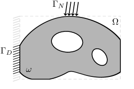
Figure 1: Illustration of the prescribed boundary conditions defined on the design domain $\Omega$. In a density formulation, each admissible shape $\omega\subseteq\Omega$ can be associated with some density function $\rho\in L^{\infty}(\Omega;\left[\delta_{\rho},1\right])$

$$a(\mathbf{u},\mathbf{v};\rho)=\ell(\mathbf{v}),\qquad\forall\mathbf{v}\in\mathcal{V}$$ (1)

where $\mathcal{V}=\{\mathbf{u}\in H^{1}(\Omega;\mathbb{R}^{d}):\mathbf{u}|_{\Gamma_{D}}=\mathbf{0}\}$ is the space of admissible displacements and

$$a(\mathbf{u},\mathbf{v};\rho)=\int_{\Omega}\rho^{p}\mathbf{C}_{0}\boldsymbol{\epsilon}(\mathbf{u}):\boldsymbol{\epsilon}(\mathbf{v})\mathrm{d}\mathbf{x},\qquad\ell(\mathbf{v})=\int_{\Gamma_{N}}\mathbf{t}\cdot\mathbf{v}\mathrm{d}s$$ (2)

are the usual energy bilinear and load linear forms. Moreover, $\boldsymbol{\epsilon}(\mathbf{u})=(\nabla\mathbf{u}+\nabla\mathbf{u}^{T})/2$ is the linearized strain tensor, $\mathbf{t}\in L^{2}(\Gamma_{N};\mathbb{R}^{d})$ is the prescribed tractions on $\Gamma_{N}$ and $\mathbf{C}_{0}$ is the elasticity tensor for the constituent material. Observe that the classical Solid Isotropic Material with Penalization (SIMP) model is used to describe the dependence of the state equation on the density field, namely that the stiffness is related to the density through the power law relation $\rho^{p}$ [6, 33, 32]. The bilinear form is continuous and also coercive provided that $\rho$ is measurable and bounded below by some small positive constant $0<\delta_{\rho}\ll 1$. In fact, there exist positive constants $c$ and $M$ such that for all $\rho\in L^{\infty}(\Omega;\left[\delta_{\rho},1\right])$,

$$\left|a(\mathbf{u},\mathbf{v};\rho)\right|\leq M\left\|\mathbf{u}\right\|_{1}\left\|\mathbf{v}\right\|_{1},\quad a(\mathbf{u},\mathbf{u};\rho)\geq c\left\|\mathbf{u}\right\|_{1}^{2},\qquad\forall\mathbf{u},\mathbf{v}\in\mathcal{V}$$ (3)

Together with continuity of the linear form $\ell$ (which follows from the assumed regularity of the applied tractions), these imply that (1) admits a unique solution $\mathbf{u}_{\rho}$ for all $\rho\in L^{\infty}(\Omega;\left[\delta_{\rho},1\right])$. Moreover, we have the uniform estimate $\left\|\mathbf{u}_{\rho}\right\|_{1}\leq c^{-1}\left\|\mathbf{t}\right\|$. For future use, we also recall that by the principle of minimum potential, $\mathbf{u}_{\rho}$ is characterized by

$$\mathbf{u}_{\rho}=\underset{\mathbf{v}\in\mathcal{V}}{\mbox{argmin}}\left[\frac{1}{2}a(\mathbf{v},\mathbf{v};\rho)-\ell(\mathbf{v})\right]$$ (4)

where the term in the bracket is the potential energy associated with deformation field $\mathbf{v}$. The following is a result that will be used later in the paper and readily follows from the stated assumptions (see, for example, [11]): Given a sequence $\left\{\rho_{n}\right\}$ and $\rho$ in $L^{\infty}(\Omega;\left[\delta_{\rho},1\right])$ such that $\rho_{n}\rightarrow\rho$ strongly in $L^{p}(\Omega),1\leq p\leq\infty$, the associate displacement fields $\mathbf{u}_{\rho_{n}}$, up to a subsequence, converge in the strong topology of $H^{1}(\Omega;\mathbb{R}^{d})$ to $\mathbf{u}_{\rho}$. This shows that if the cost functional depends continuously on $\left(\rho,\mathbf{u}\right)$ in the strong topology of $L^{p}(\Omega)\times H^{1}(\Omega;\mathbb{R}^{d})$, then compactness of the space of admissible densities in $L^{p}(\Omega)$ is a sufficient condition for existence of solutions.

The cost functional for the compliance minimization problem is given by

$$J(\rho)=\ell(\mathbf{u}_{\rho})+\lambda\int_{\Omega}\rho\mathrm{d}\mathbf{x}$$ (5)

The first term in $J$ is the compliance of the design while the second term represents a penalty on the volume of the material used. Minimizing this cost functional amounts to finding the stiffest arrangement while using the least amount of material with elasticity tensor $\mathbf{C}_{0}$. The parameter $\lambda>0$ determines the trade-off between the stiffness provided by the material and the amount that is used (which presumably is proportional to the cost of the design). Since the SIMP model assigned smaller stiffness to the intermediate densities compared to the their contribution to the volume, it is expected that in the optimal regime, the density function are nearly binary (taking only values of $\delta_{\rho}$ and 1) provided that the penalty exponent $p$ is sufficiently large.

As discussed in the introduction, the compliance minimization problem does not admit a solution unless additional restrictions are placed on the regularity of density functions. This may be accomplished by addition of a Tikhonov regularization term to the cost function [10, 41]:

$$\min_{\rho\in\mathcal{A}}\ \tilde{J}(\rho)=J(\rho)+\frac{\beta}{2}\left|\rho\right|_{1}^{2}$$ (6)

where $\beta>0$ is a positive constant determining the influence of this regularization (larger $\beta$ leads to smoother densities in the optimal regime). The minimization of $\tilde{J}$ is carried out over the set of admissible densities, defined as a subset of $H^{1}(\Omega)$, given by

$$\mathcal{A}=\left\{\rho\in H^{1}(\Omega):\delta_{\rho}\leq\rho\leq 1\mbox{ a.e.}\right\}$$ (7)

The proof of existence of minimizers for (6) can be found in [41] (see also [7] for a weaker result) and essentially follows from compactness of the minimizing sequences of (6) in $L^{p}(\Omega)$, $1\leq p<\infty$. We note that the norm of the density gradient also appears in phase field formulations of topology optimization (see, for example, [13, 17, 40]) as an interfacial energy term and is accompanied by a double-well potential penalizing intermediate densities. Taken together with appropriately chosen coefficients, the two terms serve as approximation to the perimeter of the design.

Under an additional assumption of $\partial\rho/\partial\mathbf{n}=0$ on $\partial\Omega$ and $\rho\in H^{2}(\Omega)$, the Tikhonov regularization term can be written as $\frac{1}{2}\left\langle\rho,-\beta\Delta\rho\right\rangle$. Similarly, the more general regularization term $\frac{1}{2}\left\langle\nabla\rho,\kappa\nabla\rho\right\rangle$ in which $\kappa(\mathbf{x})$ is a bounded and positive-definite matrix prescribing varying regularity of $\rho$ in $\Omega$ can be written as $\frac{1}{2}\left\langle\rho,-\nabla\cdot\left(\kappa\nabla\rho\right)\right\rangle$. For brevity and emphasizing the quadratic form of this type of regularization, in the next two sections, we write the regularizer generically as

$$\frac{1}{2}\left\langle\rho,\mathcal{R}\rho\right\rangle$$ (8)

where $\mathcal{R}$ is a linear, self-adjoint and positive semi-definite operator on $\mathcal{A}$, though the additional assumption on densities are in fact not required.

Finally, we recall that the gradient of compliance (with respect to variations of density in the $L^{2}$-metric) is given by [7]

$$J^{\prime}(\rho)=-E(\rho)+\lambda$$ (9)

where $E(\rho)=p\rho^{p-1}\mathbf{C}_{0}\boldsymbol{\epsilon}(\mathbf{u}_{\rho}):\boldsymbol{\boldsymbol{\epsilon}}(\mathbf{u}_{\rho})$ is a strain energy density field. Note that $E(\rho)$ is non-negative for any admissible density and this is related to the monotonicity of the self-adjoint compliance problem: given densities $\rho_{1}$ and $\rho_{2}$ such that $\rho_{1}\leq\rho_{2}$ a.e., one can show $\ell(\mathbf{u}_{\rho_{1}})\geq\ell(\mathbf{u}_{\rho_{2}})$. This property is the main reason why we restrict our attention in this paper to compliance minimization (though in section 7, we will provide an example of compliant mechanism design which is not self-adjoint). Observe that $\hat{\rho}$ is a stationary point of $J$ if

$$\begin{cases}E(\hat{\rho})(\mathbf{x)}<\lambda,&\mbox{if }\hat{\rho}(\mathbf{x)}=\delta_{\rho}\\ E(\hat{\rho})(\mathbf{x)}=\lambda,&\mbox{if }\delta_{\rho}<\hat{\rho}(\mathbf{x)}<1\\ E(\hat{\rho})(\mathbf{x)}>\lambda,&\mbox{if }\hat{\rho}(\mathbf{x)}=1\end{cases}$$ (10)

Thus, in regions where $E(\hat{\rho})$ exceeds the penalty parameter $\lambda$ (regions that experience “large” deformation), density is at its maximum. Similarly, below this cutoff value the density is equal to the lower bound $\delta_{\rho}$. Everywhere else, i.e., in the regions of intermediate density, the strain energy density is equal to the penalty parameter $\lambda$.

Figure 2 shows the distribution of $E(\rho)-\lambda$ for solutions to (6) obtained using the proposed algorithm (cf. section 7 and Figures 7(b) and (c)). Superimposed are the contour lines associated with $\rho=1/2$ (plotted in black) representing the boundary of the optimal shape and $E(\rho)=\lambda$ (plotted in dashed white). The fact that these lines are nearly coincident shows that the solutions to the regularized problem, at least for sufficiently small regularization parameter $\beta$, are close to ideal in the sense that they nearly satisfy the stationarity condition for the structural objective $J$.

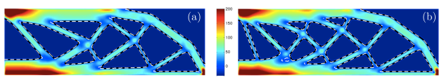
Figure 2: Plot of $E(\rho)-\lambda$ for two solutions to the MBB beam problem with $\beta=0.01$ (a) corresponds to solution shown in Figure 7(b) and (b) corresponds to solution shown in Figure 7(c). The black line is the contour line for $\rho=1/2$ and the dashed white line is the contour line where $E(\rho)=\lambda$. Note that only half the design domain is shown and the range of the colorbar is limited to $\left[-\lambda,6\lambda\right]$ for better visualization.

3 General Splitting Algorithm

In this section, we discuss a generalization of the forward-backward splitting algorithm that was explored in [41] for solving the regularized compliance minimization problem. The key idea behind this and other similar decomposition methods [20, 19, 29] is the separate treatment of constituent terms of the cost function.

A general algorithm for finding a minimizer of $\tilde{J}(\rho)$ consists of subproblems of the form:

$$\rho_{n+1}=\underset{\rho\in\mathcal{A}_{n}}{\mbox{argmin}}\ J(\rho_{n})+\left\langle\rho-\rho_{n},J^{\prime}(\rho_{n})\right\rangle+\frac{1}{2\tau_{n}}\left\|\rho-\rho_{n}\right\|_{\mathcal{H}_{n}}^{2}+\frac{1}{2}\left\langle\rho,\mathcal{R}\rho\right\rangle$$ (11)

where $\mathcal{H}_{n}$ is a bounded and positive-definite linear operator. Compared to (6), we can see that while the regularization term has remained intact, $J$ is replaced by a local quadratic model around $\rho_{n}$ in which $\mathcal{H}_{n}$ may be viewed as an approximation to the Hessian of $J$ evaluated at $\rho_{n}$. Note that constant terms such as $J(\rho_{n})$ and $\left\langle\rho_{n},J^{\prime}(\rho_{n})\right\rangle$ do not affect the optimization but are provided to emphasize the expansion of $J$. Moreover, $\tau_{n}>0$ is a step size parameter that determines the curvature of this approximation. For sufficiently small $\tau_{n}$ (large curvature), the approximation is conservative in that it majorizes (lies above) $J$, which is crucial in guaranteeing decent in each iteration and overall convergence of the algorithm (see section 6).

We have included another limiting measure in (11), a minor departure from the above-mentioned references, by replacing the constraint set $\mathcal{A}$ by a subset $\mathcal{A}_{n}$ in order to limit the point-wise change in the density to a specified move limit $m_{n}$. More specifically, we have defined

$$\mathcal{A}_{n}=\left\{\rho\in\mathcal{A}:\left|\rho-\rho_{n}\right|\leq m_{n}\mbox{ a.e.}\right\}=\left\{\rho\in H^{1}(\Omega):\rho_{n}^{\mathsf{L}}\leq\rho\leq\rho_{n}^{\mathsf{U}}\mbox{ a.e.}\right\}$$ (12)

where in the latter expression

$$\rho_{n}^{\mathsf{L}}=\delta_{\rho}\wedge\left(\rho_{n}-m_{n}\right),\quad\rho_{n}^{\mathsf{U}}=1\vee\left(\rho_{n}+m_{n}\right)$$ (13)

The presence of move limits (akin to a trust region strategy) is common in topology optimization literature as a means to stabilize the topology optimization algorithm, especially in the early iterations to prevent members from forming too prematurely. As we will show with an example, this is only important when a smaller regularization parameter is used and the final topology is complex. Near the optimal solution, the move limit strategy is typically inoperative. Of course, by setting $m_{n}\equiv 1$, we can get $\mathcal{A}=\mathcal{A}_{n}$ and recover the usual form of (11).

Ignoring the constant terms and with simple rearrangement, we can show that (11) is equivalent to

$$\rho_{n+1}=\underset{\rho\in\mathcal{A}_{n}}{\mbox{argmin}}\ \left\|\rho-\rho_{n+1}^{*}\right\|_{\left(\mathcal{H}_{n}+\tau_{n}\mathcal{R}\right)}^{2}$$ (14)

where the interim density $\rho_{n+1}^{*}$ is given by

$$\rho_{n+1}^{*}=\left(\mathcal{H}_{n}+\tau_{n}\mathcal{R}\right)^{-1}\left[\mathcal{H}_{n}\rho_{n}-\tau_{n}J^{\prime}(\rho_{n})\right]$$ (15)

Alternatively, the interim density can be written as a Newton-type update where the gradient of $\tilde{J}$ is scaled by the inverse of its approximate Hessian, namely

$$\rho_{n+1}^{*}=\rho_{n}-\tau_{n}\left(\mathcal{H}_{n}+\tau_{n}\mathcal{R}\right)^{-1}\left[J^{\prime}(\rho_{n})+\mathcal{R}\rho_{n}\right]$$ (16)

Returning to (14), we can see that next density $\rho_{n+1}$ is defined as the projection of the interim density, with respect to the norm defined by $\mathcal{H}_{n}+\tau_{n}\mathcal{R}$, onto the constraint space $\mathcal{A}_{n}$. From the assumptions on properties of $\mathcal{H}_{n}$ and the Tikhonov regularization operator $\mathcal{R}$ and the fact that $\mathcal{A}_{n}$ is a closed convex subset of $H^{1}(\Omega)$, it follows that the projection is well-defined and there is a unique update $\rho_{n+1}$.

By setting $\mathcal{R}=-\beta\Delta$, which corresponds to the regularization term of $\eqref{eq:reg-compliance}$ and choosing $\mathcal{H}_{n}$ to be the identity map $\mathcal{I}$, we recover the forward-backward algorithm investigated in [41]. In this case, the interim update satisfies the Helmholtz equation

$$\left(\mathcal{I}-\tau_{n}\beta\Delta\right)\rho_{n+1}^{*}=\rho_{n}-\tau_{n}J^{\prime}(\rho_{n})$$ (17)

with homogenous Neumann boundary conditions. Note that the right hand side is the usual gradient descent step (with step size $\tau_{n}$) associated with $J$ (the forward step) and the interim density is obtained from application of the inverse of the Helmholtz operator (the backward step), which can be viewed as the filtering of right-hand-side with the Gaussian Green’s function of the Helmholtz equation. As mentioned in the introduction, this appearance of filtering is fundamentally different from density and sensitivity filtering methods. Moreover, the projection operation in this case is with respect to a scaled Sobolev metric, namely

$$\rho_{n+1}=\underset{\rho\in\mathcal{A}_{n}}{\mbox{argmin}}\ \left\|\rho-\rho_{n+1}^{*}\right\|^{2}+\beta\tau_{n}\left|\rho-\rho_{n+1}^{*}\right|_{1}^{2}$$ (18)

which numerically requires the solution to a box-constrained convex quadratic program. In [41], we also explored an “inconsistent” variation of this algorithm where we neglected the second term in (18) and essentially used the $L^{2}$-metric for the projection step. Due to the particular geometry of the box constraints in $\mathcal{A}_{n}$, the $L^{2}$-projection has the explicit solution given by

$$\rho_{n+1}=\left(\rho_{n+1}^{*}\wedge\rho_{n}^{\mathsf{L}}\right)\vee\rho_{n}^{\mathsf{U}}$$ (19)

The appeal of this min/max type operation is that it is trivial from the computational point of view. Moreover, it coincides with the last step in the OC update scheme [7]. However, this is an inconsistent step for Tikhonov regularized problem since $\rho_{n+1}$ need not lie in $H^{1}(\Omega)$. In fact, strictly speaking, (19) is valid only if $\mathcal{A}_{n}$ is enlarged from functions in $H^{1}(\Omega)$ to all functions in $L^{2}(\Omega)$ bounded below by $\rho_{n}^{\mathsf{L}}$ and above by $\rho_{n}^{\mathsf{U}}$. In spite of this inconsistency, the algorithm composed of (17) and (19) was convergent and numerically shown to produce noteworthy solutions with minimal intermediate densities. This merits a separate investigation since as suggested in [41], this algorithm may in fact solve a smoothed version of the perimeter constraint problem where the regularization term is the total variation of the density field. We will return to the use of $L^{2}$-projection later in section 6 but this time in a consistent manner with the aid of the two-metric projection approach of [8, 24].

4 Optimality Criteria and Sensitivity Filtering

In structural optimization, the optimality criteria (OC) method is preferred to the gradient descent algorithm since it typically enjoys faster convergence (see [3] on the relationship between the two methods). Our interest here in the OC method is that the density and sensitivity filtering methods are typically implemented in the OC framework. Moreover, as we shall see, this examination will lead to the choice of $\mathcal{H}_{n}$ in the algorithm (11).

The interim density in the OC method for the compliance minimization problem (in the absence of regularization) is obtained from the fixed point iteration

$$\rho_{n+1}^{*}=\rho_{n}\left[\frac{E(\rho_{n})}{\lambda}\right]^{1/2}\equiv\rho_{n}\left[e_{\lambda}(\rho_{n})\right]^{1/2}$$ (20)

Note that the strain energy density $E(\rho_{n})$ and subsequently its normalization $e_{\lambda}(\rho_{n})$ are non-negative for any admissible density $\rho_{n}$ and therefore $\rho_{n+1}^{*}$ is well-defined. Recalling the necessary condition of optimality for an optimal density $\hat{\rho}$ stated in (10), it is evident that such $\hat{\rho}$ is a fixed point of the OC iteration. Intuitively, the current density $\rho_{n}$ is increased (decreased) in regions where $E(\rho_{n})$ is greater (less) than the penalty parameter $\lambda$ by a factor of $\left[e_{\lambda}(\rho_{n})\right]^{1/2}$. The next density $\rho_{n+1}$ in the OC is given by (19).

It is more useful here to adopt an alternative view of the OC scheme, namely that the OC update can be seen as the solution to an approximate subproblem where compliance is replaced by a Taylor expansion in the intermediate field $\rho^{-1}$ [25]. The intuition behind such expansion is that locally compliance is inversely proportional to density. In particular, $\rho_{n+1}^{*}$ can be shown to be the stationary point of the “reciprocal approximation” around $\rho_{n}$ defined by

$$J_{\mathsf{rec}}(\rho;\rho_{n})\equiv\ell(\mathbf{u}_{\rho_{n}})+\left\langle\frac{\rho_{n}}{\rho}\left(\rho-\rho_{n}\right),-E(\rho_{n})\right\rangle+\lambda\int_{\Omega}\rho\mathrm{d}\mathbf{x}$$ (21)

Note that the expansion in the inverse of density is carried out only for the compliance term, and the volume term, which is already linear, is not altered. The expression for $J_{\mathsf{rec}}(\rho;\rho_{n})$ can be alternatively written as

$$J_{\mathsf{rec}}(\rho;\rho_{n})=J(\rho_{n})+\left\langle\rho-\rho_{n},J^{\prime}(\rho_{n})\right\rangle+\frac{1}{2}\left\langle\rho-\rho_{n},\frac{2E(\rho_{n})}{\rho}\left(\rho-\rho_{n}\right)\right\rangle$$ (22)

which highlights the fact that the (nonlinear) curvature term in (22) makes it a more accurate approximation of compliance compared to the linear expansion. With regard to the OC update, one can show that the interim update satisfies $J^{\prime}_{\mathsf{rec}}(\rho_{n+1}^{*};\rho_{n})=0$, and its $L^{2}$-projection is indeed the minimizer of $J_{\mathsf{rec}}(\rho;\rho_{n})$ over $\mathcal{A}_{n}$ (again enlarged to $L^{2}$).

We now turn to the sensitivity filtering method, which is described with the OC algorithm. Let $\mathcal{F}$ denote a linear filtering map, for example, the Helmholtz filter $\mathcal{F}=\left(\mathcal{I}-r^{2}\Delta\right)^{-1}$ discussed before or the convolution filter of radius radius $r$ [12, 11]

$$\mathcal{F}(\psi)(\mathbf{x})\equiv\int_{\Omega}F_{r}(\mathbf{x}-\mathbf{y})\psi(\mathbf{y})\mathrm{d}\mathbf{y}$$ (23)

where the kernel is the linear hat function $F_{r}(\mathbf{x})=\max\left(1-\left|\mathbf{x}\right|/r,0\right)$. The main idea in the sensitivity filtering method is that $e_{\lambda}(\rho_{n})$ is heuristically replaced by the following smoothed version

$$\tilde{e}_{\lambda}(\rho_{n})\equiv\frac{1}{\rho_{n}}\mathcal{F}\left[\rho_{n}e_{\lambda}(\rho_{n})\right]$$ (24)

before entering the OC update. The interim density update is thus given by

$$\rho_{n+1}^{*}=\rho_{n}\left[\tilde{e}_{\lambda}(\rho_{n})\right]^{1/2}=\rho_{n}\left\{\frac{\mathcal{F}\left[\rho_{n}e_{\lambda}(\rho_{n})\right]}{\rho_{n}}\right\}^{1/2}=\rho_{n}^{1/2}\mathcal{F}\left[\rho_{n}e_{\lambda}(\rho_{n})\right]^{1/2}$$ (25)

A key observation in this work is that if we replace the gradient decent step in forward-backward algorithm (cf. (17)) with the OC step, we obtain a similar update scheme to that of the sensitivity filtering method. More specifically, note that (17) can be written as $\rho_{n+1}^{*}=\mathcal{F}\left[\rho_{n}-\tau_{n}J^{\prime}(\rho_{n})\right]$. Substituting the term in the bracket with $\rho_{n}\left[e(\rho_{n})\right]^{1/2}$ gives

$$\rho_{n+1}^{*}=\mathcal{F}\left\{\rho_{n}\left[e_{\lambda}(\rho_{n})\right]^{1/2}\right\}$$ (26)

which resembles (25). In fact, as illustrated in Figure 3, the two expressions produce very similar final results (in particular, observe the similarity between the patches of intermediate density in the corners that is characteristic of the sensitivity filtering method). Of course, the leap from the forward-backward algorithm to (26), just like the sensitivity filtering method, lacks mathematical justification. However, we will expand upon this observation and next derive the algorithm similar to this empirical modification of the forward-backward algorithm in a consistent manner.

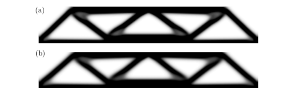
Figure 3: (a) The solution to the MBB beam problem (see section 6) using the sensitivity filtering method (consisting of (25) and (19)) (b) The solution using the update steps (26) and (19). In both cases, $\mathcal{F}$ is taken to be the “Helmholtz” filter and the move limit was set to $m_{n}=0.25$

Embedding the Reciprocal Approximation

Recalling the role of the reciprocal approximation of compliance in the OC method, the key idea is to embed such an approximation in the general subproblem of (11). We do so by choosing $\mathcal{H}_{n}$ to be the Hessian of $J_{\mathsf{rec}}(\rho;\rho_{n})$ evaluated at $\rho_{n}$, namely

$$\mathcal{H}_{n}=J_{\mathsf{rec}}^{\prime\prime}(\rho_{n};\rho_{n})=\frac{2E(\rho_{n})}{\rho_{n}}\mathcal{I}$$ (27)

As noted earlier, $E(\rho)$ is a non-negative function for any admissible $\rho$ but may vanish in some subset of $\Omega$. This means that $\mathcal{H}_{n}$ is only positive semi-definite and does not satisfy the definiteness requirement for use in (11). We can remedy this by replacing $E(\rho_{n})$ in (27) with $E(\rho_{n})\wedge\delta_{E}$ where $0<\delta_{E}\ll\lambda$ is a prescribed constant. However, in most compliance problems (e.g., the benchmark problem considered later in section 7) the strain energy field is strictly positive for all admissible densities. In fact, the regions with zero strain energy density do not experience any deformation and in light of the conditions of optimality (10) should be assigned the minimum density. Therefore, to simplify the matters, we assume in the remainder of this section that the loading and support conditions defined on $\Omega$ are such that $E(\rho)\geq\delta_{E}$ almost everywhere for all $\rho\in L^{\infty}(\Omega;\left[\delta_{\rho},1\right])$.

Comparing the quadratic approximation of $J$ with this choice of $\mathcal{H}_{n}$ and the reciprocal approximation itself (cf. (22)), we see that the difference is in their curvature terms (the linear terms of course match). The curvature of the quadratic model depends on and can be controlled by $\tau_{n}$ while the nonlinear curvature in $J_{\mathrm{rec}}$ is a function of $\rho$.

Substituting (27) into (15), the expression for the interim density becomes

$$\left[\frac{2E(\rho_{n})}{\rho_{n}}\mathcal{I}+\tau_{n}\mathcal{R}\right]\rho_{n+1}^{*}=2E(\rho_{n})+\tau_{n}\left[E(\rho_{n})-\lambda\right]=\left(2+\tau_{n}\right)E(\rho_{n})-\tau_{n}\lambda$$ (28)

Multiplying by $\rho_{n}/\left[2E(\rho_{n})\right]$ and simplifying yields

$$\left[\mathcal{I}+\frac{\rho_{n}}{2E(\rho_{n})}\tau_{n}\mathcal{R}\right]\rho_{n+1}^{*}=\rho_{n}\left[\left(1+\frac{\tau_{n}}{2}\right)-\frac{\tau_{n}}{2e_{\lambda}(\rho_{n})}\right]$$ (29)

To better understand the characteristics of this update, let us specialize to the case of Tikhonov regularization and set $\tau_{n}=1$ (so that the quadratic model and the reciprocal approximation have the same curvature at $\rho_{n}$). This gives

$$\left[\mathcal{I}-\frac{\rho_{n}}{2E(\rho_{n})}\beta\Delta\right]\rho_{n+1}^{*}=\rho_{n}\left[\frac{3}{2}-\frac{1}{2e_{\lambda}(\rho_{n})}\right]$$ (30)

First note that in the absence of regularization (i.e., $\beta=0$), the update relation has the same fixed-point iteration form as the OC update with the ratio $e_{\lambda}(\rho_{n})$ determining the scaling of $\rho_{n}$. The scaling field here is $3/2-1/\left[2e_{\lambda}(\rho_{n})\right]$ whereas in the OC method it is given by $\left[e_{\lambda}(\rho_{n})\right]^{1/2}$. As shown in Figure 4, the scaling fields and their derivatives coincide in the regions where $e_{\lambda}(\rho_{n})=1$, which means that locally the two are similar. The reduction in density is more aggressive with this scaling when $e_{\lambda}(\rho_{n})<1$ whereas the OC update leads to larger increase for $e_{\lambda}(\rho_{n})>1$.

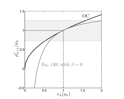
Figure 4: Comparison between scaling terms appearing in the OC update and right hand side of (30). The OC is more aggressive in regions $e_{\lambda}(\rho_{n})>1$ and less aggressive when $e_{\lambda}(\rho_{n})<1$.

As with the forward-backward algorithm (cf. equation (17)), the presence of regularization again leads to the appearance of Helmholtz filtering (the inverse of left-hand-side operator) but with two notable differences. First, the right-hand-side term now is an OC-like scaling of density instead of the gradient descent step (the same is true in (29) for an arbitrary step size $\tau_{n}$). Furthermore, the filtering is not uniform across the domain and its degree of smoothening is scaled by $\rho_{n}/\left[2E(\rho_{n})\right]$. The important result here is that, by embedding the reciprocal approximation of compliance in our quadratic model, we are able to obtain a relation for the $\rho_{n+1}^{*}$ that features an OC-like right-hand-side and its filtering, very much similar in form to the (heuristically) fabricated update scheme of (26) that was compared to the sensitivity filtering.

Another key difference between the forward-backward algorithm and the OC-based filtering methods is that the projection of $\rho_{n+1}^{*}$ defining the next iterate $\rho_{n+1}$ in the forward-backward scheme is with respect to the metric induced by $\mathcal{H}_{n}+\tau_{n}\mathcal{R}$ in contrast to the $L^{2}$-projection given by (19). As discussed before, the $L^{2}$-projection is well-suited for the geometry of the constraint set $\mathcal{A}_{n}$ due to decomposition of box constraints. It may be tempting to inconsistently use the interim density (29) with the $L^{2}$-projection but this is not necessarily guaranteed to decrease the cost function. Arbitrary projections of unconstrained Newton steps is not mathematically warranted.

In section 6, we explore a variant of the splitting algorithm that is related to the two-metric projection method of [8, 24], and allows for the use of a more convenient metric for the projection step. This can be done provided that the operator whose associated norm defines the gradient is modified appropriately in the regions where the constraints are active. More specifically, in the interim update step (cf. (16)), $\mathcal{H}_{n}+\tau_{n}\mathcal{R}$ is modified to produce a linear operator $\mathcal{D}_{n}$ with a particular structure that eliminates the coupling between regions of active and free constraints. The projection of the interim density given by

$$\rho_{n+1}^{*}=\rho_{n}-\tau_{n}\mathcal{D}_{n}^{-1}\left[J^{\prime}(\rho_{n})+\mathcal{R}\rho_{n}\right]$$ (31)

with respect to the $L^{2}$-norm is then guaranteed to decrease the cost function. Note that when there are no active constraints (e.g., in the beginning of the algorithm the density field takes mostly intermediate values), $\mathcal{D}_{n}=\mathcal{H}_{n}+\tau_{n}\mathcal{R}$ and (29) holds for the interim update and its $L^{2}$-projection produces the next iterate. In general, (29) holds locally for the regions where the box constraints are not active (i.e., regions of intermediate density) and so the analogy to the sensitivity filtering method holds in such regions.

To avoid some technical nuisances (that the $L^{2}$-projection on $H^{1}(\Omega)$ is not well-defined) and avoid the cumbersome notation required to precisely define $\mathcal{D}_{n}$ in the continuum setting (that may obscure the simple procedure for its construction), we defer the details to section 6 where we describe the algorithm for the finite-dimensional optimization problem obtained from the usual finite element approximation procedure. The intuition developed in the preceding discussion carries over to the discrete setting.

5 Finite Element Approximation

We begin with describing the approximate “finite element” optimization problem, based on a typical choice of discretization spaces, and establish the convergence of the corresponding optimal solutions to a solution of the continuum problem (6) in the limit of mesh refinement. Our result proves strong convergence of a subsequence of solutions, and therefore rules out the possibility of numerical instabilities such as checkerboard patterns observed in density-based methods. We remark that similar results are available for the density-based restriction formulations (see for example [31, 30, 12]) and the proof is along the same lines. Such convergence results are essential in justifying an overall optimization approach where one first discretizes a well-posed continuum problem and then chooses an algorithm to solve the resulting finite dimensional problem (this is the procedure adopted in this work). Then, with the FE convergence result in hand, the only remaining task is to analyze the convergence of the proposed optimization algorithm, which is discussed in the section 6.

5.1 Convergence under mesh refinement

Consider partitioning of $\Omega$ into pairwise disjoint finite elements $\mathcal{T}_{h}=\left\{\Omega_{e}\right\}_{e=1}^{l}$ with characteristic mesh size $h$. Let $\mathcal{A}_{h}$ be the FE subspace of $\mathcal{A}$ based on this partition:

$$\mathcal{A}_{h}=\left\{\rho\in C^{0}(\overline{\Omega}):\rho|_{\Omega_{e}}\in\mathcal{P}(\Omega_{e}),\forall e=1,\dots,l\right\}\cap\mathcal{A}$$ (32)

where $\mathcal{P}(\Omega_{e})$ is a space of polynomial (rational in the case of polygonal elements) functions defined on $\Omega_{e}$. Similarly, we define:

$$\mathcal{V}_{h}=\left\{\mathbf{u}\in C^{0}(\overline{\Omega};\mathbb{R}^{d}):\left[\mathbf{u}\right]_{i}|_{\Omega_{e}}\in\mathcal{P}(\Omega_{e}),\forall e=1,\dots,l,\forall i=1,\dots,d\right\}\cap\mathcal{V}$$ (33)

We also assume that the mesh $\mathcal{T}_{h}$ is chosen in such a way that the transition from $\Gamma_{D}$ to $\Gamma_{N}$ is properly aligned with the mesh. In practice, both density and displacement fields are discretized with linear elements (e.g., linear triangles, bilinear quads or linearly-complete convex polygons in two spatial dimensions). To avoid any ambiguity regarding the definition of the FE partitions, we assume a regular refinement of the meshes such that the resulting finite element spaces are ordered, e.g., $\mathcal{A}_{h}\supseteq\mathcal{A}_{h^{\prime}}$ whenever $h\leq h^{\prime}$. We consider the limit $h\rightarrow 0$ to establish convergence of solutions under mesh refinement.

What is needed in the proof of convergence is the existence of an interpolation operator $\mathcal{I}_{h}:\mathcal{V}\rightarrow\mathcal{V}_{h}$ such that for all $\mathbf{u}\in\mathcal{V}\cap H^{2}(\Omega;\mathbb{R}^{d})$

$$\left\|\mathcal{I}_{h}\mathbf{u}-\mathbf{u}\right\|_{1}\leq Ch\left|\mathbf{u}\right|_{2}$$ (34)

which in turn shows that $\mathcal{I}_{h}\mathbf{u}\rightarrow\mathbf{u}$ as $h\rightarrow 0$. Similarly, we need the mapping $i_{h}:\mathcal{A}\rightarrow\mathcal{A}_{h}$ for the design space such that $i_{h}\rho\rightarrow\rho$ as $h\rightarrow 0$. The construction of such interpolants is standard in finite element approximation theory, see for example [15].

The approximate finite element problem, specialized to Tikhonov regularization, is defined by

$$\min_{\rho\in\mathcal{A}_{h}}\tilde{J}_{h}(\rho):=J_{h}(\rho)+\frac{\beta}{2}\left|\rho\right|_{1}^{2}$$ (35)

where $J_{h}(\rho):=\ell(\mathbf{u}_{\rho,h})+\lambda\int_{\Omega}\rho\mathrm{d}\mathbf{x}$ and $\mathbf{u}_{\rho,h}$ is the solution to the Galerkin approximation of (1) given by

$$a(\mathbf{u}_{h},\mathbf{v}_{h};\rho)=\ell(\mathbf{v}_{h}),\qquad\forall\mathbf{v}_{h}\in\mathcal{V}_{h}$$ (36)

By the principle of minimum potential, we can write

$$\ell(\mathbf{u}_{\rho,h})=-2\min_{\mathbf{v}_{h}\in\mathcal{V}_{h}}\left[\frac{1}{2}a(\mathbf{v}_{h},\mathbf{v}_{h};\rho)-\ell(\mathbf{v}_{h})\right]=\max_{\mathbf{v}_{h}\in\mathcal{V}_{h}}\left[2\ell(\mathbf{v}_{h})-a(\mathbf{v}_{h},\mathbf{v}_{h};\rho)\right]$$ (37)

From the above relation, it is easy to see that $\mathcal{V}_{h}\subseteq\mathcal{V}$ implies $\ell(\mathbf{u}_{\rho,h})\leq\ell(\mathbf{u}_{\rho})$ for any given $\rho$, and therefore

$$\tilde{J}_{h}(\rho)\leq\tilde{J}(\rho)$$ (38)

that is, the finite approximation of the state equation leads to a smaller computed value of the cost function for any density field.

Consider a sequence of FE partitions $\mathcal{T}_{h}$ with $h\rightarrow 0$ and let $\rho_{h}$ be the optimal solution to the associated finite element approximation (35), i.e., minimizer of $\tilde{J}_{h}$ in $\mathcal{A}_{h}$. We first show the sequence $\rho_{h}$ is bounded in $H^{1}(\Omega)$. To see this, fix $h_{0}$ in this sequence. If $\hat{\rho}_{h}$ is the minimizer of $\tilde{J}$ in $\mathcal{A}_{h}$ (there is no approximation of the displacement field involved here), then

$$\tilde{J}(\hat{\rho}_{h})\leq\tilde{J}(\rho_{h_{0}})$$ (39)

since $\rho_{h_{0}}\in\mathcal{A}_{h_{0}}\subseteq\mathcal{A}_{h}$. Now, from the definition of $\rho_{h}$ and (38), we have $\tilde{J}_{h}(\rho_{h})\leq\tilde{J}_{h}(\hat{\rho}_{h})\leq\tilde{J}(\hat{\rho}_{h})$ and so

$$\tilde{J}_{h}(\rho_{h})\leq\tilde{J}(\rho_{h_{0}})=\tilde{J}_{h_{0}}(\rho_{h_{0}})+\left[J(\rho_{h_{0}})-J_{h_{0}}(\rho_{h_{0}})\right]:=\tilde{J}_{h_{0}}(\rho_{h_{0}})+\epsilon_{h_{0}}$$ (40)

where $\epsilon_{h_{0}}$ is the finite element error in computing compliance of $\rho_{h_{0}}$ on mesh $\mathcal{T}_{h_{0}}$. Since (40) holds for all $h\leq h_{0}$, we conclude that

$$\limsup_{h\rightarrow 0}\tilde{J}_{h}(\rho_{h})\leq\tilde{J}_{h_{0}}(\rho_{h_{0}})+\epsilon_{h_{0}}$$ (41)

Both the compliance and volume terms in $\tilde{J}_{h}(\rho_{h})$ are uniformly bounded, and so (41) shows $\limsup_{h}\left|\rho_{h}\right|_{1}^{2}<\infty$ . Thus the sequence $\rho_{h}$ is bounded in $H^{1}(\Omega)$. By Rellich’s theorem Evans [23], we have convergence of a subsequence, again denoted by $\left\{\rho_{h}\right\}$, strongly in $L^{2}(\Omega)$ and weakly in $H^{1}(\Omega)$ to some $\rho^{*}\in\mathcal{A}$. We next show that $\rho^{*}$ is a solution to continuum problem, thereby establishing the convergence of the FE approximate problem. First note that by lower semi-continuity of the norm under weak convergence,

$$\left|\rho^{*}\right|_{1}^{2}\leq\liminf_{h}\left|\rho_{h}\right|_{1}^{2}$$ (42)

Furthermore, to show convergence of $\mathbf{u}_{\rho_{h},h}$ to $\mathbf{u}_{\rho^{*}}$ in $H^{1}(\Omega;\mathbb{R}^{d})$, first note that the convergence results stated in section 2 implies that up to a subsequence $\mathbf{u}_{\rho_{h}}\rightarrow\mathbf{u}_{\rho^{*}}$ as $h\rightarrow 0$. Moreover,

$$\left\|\mathbf{u}_{\rho^{*}}-\mathbf{u}_{\rho_{h},h}\right\|_{1} \leq \left\|\mathbf{u}_{\rho^{*}}-\mathbf{u}_{\rho_{h}}\right\|_{1}+\left\|\mathbf{u}_{\rho_{h}}-\mathbf{u}_{\rho_{h},h}\right\|_{1}$$

$$\leq \left\|\mathbf{u}_{\rho^{*}}-\mathbf{u}_{\rho_{h}}\right\|_{1}+\frac{M}{c}\left\|\mathbf{u}_{\rho_{h}}-\mathcal{I}_{h}(\mathbf{u}_{\rho_{h}})\right\|_{1}$$

$$\leq \left\|\mathbf{u}_{\rho^{*}}-\mathbf{u}_{\rho_{h}}\right\|_{1}+\hat{C}h\left|\mathbf{u}_{\rho_{h}}\right|_{2}$$

where the second inequality follows from Cea’s lemma [15] and last inequality follows from estimate (34). Hence $\mathbf{u}_{\rho_{h},h}\rightarrow\mathbf{u}_{\rho^{*}}$ in $H^{1}(\Omega;\mathbb{R}^{d})$ and so $J_{h}(\rho_{h})\rightarrow J(\rho^{*})$. Together with the above inequality, we have

$$\tilde{J}(\rho^{*})\leq\liminf_{h}\tilde{J}_{h}(\rho_{h})$$ (44)

To establish optimality of $\rho^{*}$, take any $\rho\in\mathcal{A}_{h}$. The definition of $\rho_{h}$ as the optimal solution to (35) implies

$$\tilde{J_{h}}(\rho_{h})\leq\tilde{J_{h}}\left[i_{h}(\rho)\right]$$ (45)

Using a similar argument as above, we can pass (45) to the limit to show $\tilde{J}(\rho^{*})\leq\tilde{J}(\rho)$.

5.2 The Discrete Problem

We proceed to obtain explicit expressions for the discrete problem (35) for a given finite element partition $\mathcal{T}_{h}$. For each $\rho_{h}\in\mathcal{A}_{h}$, we have the expansion $\rho_{h}(\mathbf{x})=\sum_{k=1}^{m}\left[\mathbf{z}\right]_{k}\varphi_{k}(\mathbf{x})$ where $\mathbf{z}$ is the vector of nodal densities characterizing $\rho_{h}$ and $\left\{\varphi_{k}\right\}_{k=1}^{m}$ the set of finite element basis functions for $\mathcal{A}_{h}$. The finite-dimensional space corresponding to $\mathcal{A}_{h}$ is simply the closed cube $\left[\delta_{\rho},1\right]^{m}$. Moreover, the vector form for the Tikhonov regularization term is

$$\frac{\beta}{2}\left|\rho_{h}\right|_{1}^{2}=\frac{1}{2}\mathbf{z}^{T}\mathbf{G}\mathbf{z}$$ (46)

where $\mathbf{G}$ is the usual finite element matrix defined by $\left[\mathbf{G}\right]_{k\ell}=\beta\int_{\Omega}\nabla\varphi_{k}\cdot\nabla\varphi_{\ell}\mathrm{d}\mathbf{x}$, which is positive semi-definite. Similarly, the volume term $\int_{\Omega}\rho\mathrm{d}\mathbf{x}$ can be written as $\mathbf{z}^{T}\mathbf{v}$ where $\left[\mathbf{v}\right]_{k}=\int_{\Omega}\varphi_{k}\mathrm{d}\mathbf{x}$.

With regard to state equation (36), we make one approximation in the energy bilinear form by assuming that the density field has a constant value over each element, equal to the centroidal value, in the bilinear form. If $\mathbf{x}_{e}$ denotes the location of the centroid of element $\Omega_{e}$, we replace each $\rho_{h}(\mathbf{x})$ by

$$\sum_{e=1}^{l}\chi_{\Omega_{e}}(\mathbf{x})\rho_{h}(\mathbf{x}_{e})$$ (47)

in the state equation. The use of piecewise element density is common practice in topology optimization (cf. [43]) and makes the calculations and notation simpler. If $\left\{\mathbf{N}_{i}\right\}_{i=1}^{q}$ denotes the basis functions for the displacement field such that $\mathbf{u}_{h}(\mathbf{x})=\sum_{i=1}^{q}\mathbf{\left[U\right]}_{i}\mathbf{N}_{i}(\mathbf{x})$, the vector form of (36) is given by

$$\mathbf{K}\mathbf{U}=\mathbf{F}$$ (48)

where the load vector $\left[\mathbf{F}\right]_{i}=\int_{\Gamma_{N}}\mathbf{t}\cdot\mathbf{N}_{i}\mathrm{d}s$ and the stiffness matrix, with the above approximation of density, is

$$\left[\mathbf{K}\right]_{ij}=\int_{\Omega}\rho_{h}^{p}\mathbf{C}_{0}\nabla\mathbf{N}_{i}:\nabla\mathbf{N}_{j}\mathrm{d}\mathbf{x}=\sum_{e=1}^{l}\left[\rho_{h}(\mathbf{x}_{e})\right]^{p}\int_{\Omega_{e}}\mathbf{C}_{0}\nabla\mathbf{N}_{i}:\nabla\mathbf{N}_{j}\mathrm{d}\mathbf{x}$$ (49)

Let us define the matrix $\mathbf{P}$ whose $\left(e,k\right)$-entry is given by $\mathbf{\left[P\right]}_{ek}=\varphi_{k}(\mathbf{x}_{e})$. Then

$$\rho_{h}(\mathbf{x}_{e})=\sum_{k=1}^{m}\varphi_{k}(\mathbf{x}_{e})\left[\mathbf{z}\right]_{k}=\sum_{k=1}^{m}\mathbf{\left[P\right]}_{ek}\left[\mathbf{z}\right]_{k}=\left[\mathbf{P}\mathbf{z}\right]_{e}$$ (50)

The vector $\mathbf{P}\mathbf{z}$ thus gives the vector of elemental density values. Returning to (49) and denoting the element stiffness matrix by $\mathbf{k}_{e}=\int_{\Omega_{e}}\mathbf{C}_{0}\nabla\mathbf{N}_{i}:\nabla\mathbf{N}_{j}\mathrm{d}\mathbf{x}$, we have the simplified expression for the global stiffness matrix

$$\mathbf{K}(\mathbf{z})=\sum_{e=1}^{l}\left(\left[\mathbf{P}\mathbf{z}\right]_{e}\right)^{p}\mathbf{k}_{e}$$ (51)

The summation effectively represents the assembly routine in practice. We note the continuity and ellipticity of the bilinear form (cf. (3)) and non-degeneracy of the finite element partition imply that the eigenvalues of $\mathbf{K}(\mathbf{z})$ are bounded below by $c_{h}$ and above by $M_{h}$ (which depend on the mesh size – see chapter 9 of [15]) for all admissible density vectors $\mathbf{z}\in\left[\delta_{\rho},1\right]^{m}$.

The discrete optimization problem (35) can now be equivalently written as (with a slight abuse of notation for $J$ and $\tilde{J}$ )

$$\min_{\mathbf{z}\in\left[\delta_{\rho},1\right]^{m}}\tilde{J}(\mathbf{z}):=J(\mathbf{z})+\frac{1}{2}\mathbf{z}^{T}\mathbf{G}\mathbf{z}$$ (52)

where

$$J(\mathbf{z})=\mathbf{F}^{T}\mathbf{U}(\mathbf{z})+\lambda\mathbf{z}^{T}\mathbf{v}$$ (53)

and $\mathbf{U(\mathbf{z})}$ is the solution to $\mathbf{K}(\mathbf{z})\mathbf{U}=\mathbf{F}$. Observe that matrices $\mathbf{P}$ and $\mathbf{G}$, the vector $\mathbf{v}$, as well as the element stiffness matrices $\mathbf{k}_{e}$ and load vector $\mathbf{F}$ are all fixed and do not change in the course of optimization. Thus they can be computed once in the beginning and stored.

The gradient of $J$ with respect to the nodal densities $\mathbf{z}$ can readily computed as

$$\partial_{k}J(\mathbf{z})=-\mathbf{U}(\mathbf{z})^{T}\left(\partial_{k}\mathbf{K}\right)\mathbf{U(\mathbf{z})}+\lambda\mathbf{\left[v\right]}_{k}$$ (54)

The expression for $\partial_{k}\mathbf{K}$ can be obtained from (51). Defining the vector of strain energy densities $\left[\mathbf{E}(\mathbf{z})\right]_{e}=p\left[\mathbf{P}\mathbf{z}\right]_{e}^{p-1}\mathbf{U}(\mathbf{z})^{T}\mathbf{k}_{e}\mathbf{U}(\mathbf{z})$, we have

$$\nabla J(\mathbf{z})=-\mathbf{P}^{T}\mathbf{E}(\mathbf{z})+\lambda\mathbf{v}$$ (55)

With the first order gradient information in hand, we can find the reciprocal approximation of compliance about point $\mathbf{y}$ as

$$J_{\mathsf{rec}}(\mathbf{z};\mathbf{y})\equiv J(\mathbf{y})+\lambda\left(\mathbf{z}-\mathbf{y}\right)^{T}\mathbf{v}+\sum_{k=1}^{m}\left(\frac{\left[\mathbf{y}\right]_{k}}{\left[\mathbf{z}\right]_{k}}\right)\left(\left[\mathbf{z}\right]_{k}-\left[\mathbf{y}\right]_{k}\right)\left[-\mathbf{P}^{T}\mathbf{E}(\mathbf{y})\right]_{k}$$ (56)

The Hessian of $J_{\mathsf{rec}}(\mathbf{z};\mathbf{y})$, evaluated at $\mathbf{z}=\mathbf{y}$, is a diagonal matrix with entries

$$h_{k}(\mathbf{y})=\partial_{kk}J_{\mathsf{rec}}(\mathbf{y};\mathbf{y})=\frac{2}{\left[\mathbf{y}\right]_{k}}\left[\mathbf{P}^{T}\mathbf{E}(\mathbf{y})\right]_{k},\quad k=1,\dots,m$$ (57)

The entries of the vector $\mathbf{E}(\mathbf{y})$ are non-negative for all admissible nodal densities but can be zero and therefore Hessian of $J_{\mathsf{rec}}(\mathbf{z};\mathbf{y})$ is only positive semi-definite.

6 Algorithms for the Discrete Problem

We begin with the generalization of the forward-backward algorithm for solving the discrete problem (52) before discussing the two-metric projection variation. As in section 3, we consider a splitting algorithm with iterations of the form

$$\mathbf{z}_{n+1}=\underset{\mathbf{z}_{n}^{\mathsf{L}}\leq\mathbf{z}\leq\mathbf{z}_{n}^{\mathsf{U}}}{\mbox{argmin}}\ Q_{J}(\mathbf{z};\mathbf{z}_{n},\tau_{n})+\frac{1}{2}\mathbf{z}^{T}\mathbf{G}\mathbf{z}$$ (58)

where, compared to (52), the regularization term is unchanged while $J$ is replaced by the following local quadratic model around current iterate $\mathbf{z}_{n}$

$$Q_{J}(\mathbf{z};\mathbf{z}_{n},\tau_{n})=J(\mathbf{z}_{n})+\left(\mathbf{z}-\mathbf{z}_{n}\right)^{T}\nabla J(\mathbf{z}_{n})+\frac{1}{2\tau_{n}}\left\|\mathbf{z}-\mathbf{z}_{n}\right\|_{\mathbf{H}_{n}}^{2}$$ (59)

The move limit constraint is accounted for through the bounds

$$\left[\mathbf{z}_{n}^{\mathsf{L}}\right]_{k}=\max\left(\delta_{\rho},\left[\mathbf{z}_{n}\right]_{k}-m_{n}\right),\quad\left[\mathbf{z}_{n}^{\mathsf{U}}\right]_{k}=\min\left(1,\left[\mathbf{z}_{n}\right]_{k}+m_{n}\right),\qquad k=1,\dots,m$$ (60)

In order to embed the curvature information from the reciprocal approximation (56) in the quadratic model, we choose

$$\mathbf{H}_{n}=\mbox{diag}(\hat{h}_{1}(\mathbf{z}_{n}),\dots,\hat{h}_{m}(\mathbf{z}_{n}))$$ (61)

where $\hat{h}_{k}(\mathbf{z}_{n})\equiv\max(h_{k}(\mathbf{z}_{n}),\delta_{E})$ and, as defined before, $0<\delta_{E}\ll\lambda$ is a small positive constant. This modification not only ensures that $\mathbf{H}_{n}$ is positive definite but also that the eigenvalues of $\mathbf{H}_{n}$ are uniformly bounded above and below, a condition that is useful for the proof of convergence of the algorithm [9]. Observe that for all $\mathbf{z}\in\left[\delta_{\rho},1\right]^{m}$,

$$0\leq h_{k}(\mathbf{z})\leq 2\delta_{\rho}^{-1}\left\|\mathbf{E}(\mathbf{z})\right\|_{\infty}\leq 2p\delta_{\rho}^{-p-1}M_{h}\left\|\mathbf{U}(\mathbf{z})\right\|^{2}\leq 2p\delta_{\rho}^{-p-1}M_{h}c_{h}^{-2}\left\|\mathbf{F}\right\|^{2}$$ (62)

where we used the fact that $\mathbf{U}^{T}\mathbf{k}_{e}\mathbf{U}\leq\delta_{\rho}^{-p}\mathbf{U}^{T}\mathbf{K}(\mathbf{z})\mathbf{U}\leq\delta_{\rho}^{-p}M_{h}\left\|\mathbf{U}(\mathbf{z})\right\|^{2}$ and that the eigenvalues of $\mathbf{K}^{-1}$ are bounded above by $c_{h}^{-1}$.

The step size parameter $\tau_{n}$ in (58) must be sufficiently small so that the quadratic model is a conservative approximation and majorizes $J$. If $\tau_{n}>0$ is chosen so that the update $\mathbf{z}_{n+1}$ satisfies

$$J(\mathbf{z}_{n+1})\leq Q_{J}(\mathbf{z}_{n+1};\mathbf{z}_{n},\tau_{n})$$ (63)

then one can show [9]

$$\tilde{J}(\mathbf{z}_{n})-\tilde{J}(\mathbf{z}_{n+1})\geq\frac{1}{2\tau_{n}}\left\|\mathbf{z}_{n}-\mathbf{z}_{n+1}\right\|_{\mathbf{H}_{n}}^{2}$$ (64)

If $\mathbf{z}_{n}$ is a stationary point of $\tilde{J}$, that is $(\mathbf{z}-\mathbf{z}_{n})^{T}\nabla\tilde{J}(\mathbf{z}_{n})\geq 0$ for all $\mathbf{z}\in\left[\delta_{\rho},1\right]^{m}$, then $\mathbf{z}_{n+1}=\mathbf{z}_{n}$ for all $\tau_{n}>0$. To see this, we write (58) equivalently as

$$\min_{\mathbf{z}_{n}^{\mathsf{L}}\leq\mathbf{z}\leq\mathbf{z}_{n}^{\mathsf{U}}}(\mathbf{z}-\mathbf{z}_{n})^{T}\nabla\tilde{J}(\mathbf{z}_{n})+\frac{1}{2\tau_{n}}\left\|\mathbf{z}-\mathbf{z}_{n}\right\|_{\mathbf{H}_{n}+\tau_{n}\mathbf{G}}^{2}$$ (65)

Since $\mathbf{H}_{n}+\tau_{n}\mathbf{G}$ is positive definite and $\mathbf{z}_{n}$ is a stationary point, the objective function is strictly positive for all $\mathbf{z}\in\left[\mathbf{z}_{n}^{\mathsf{L}},\mathbf{z}_{n}^{\mathsf{U}}\right]$ with $\mathbf{z}\neq\mathbf{z}_{n}$ while it vanishes at $\mathbf{z}_{n}$, thereby establishing optimality of $\mathbf{z}_{n}$ for subproblem (58). Otherwise, if $\mathbf{z}_{n}$ is not a stationary point of $\tilde{J}$, then $\mathbf{z}_{n+1}\neq\mathbf{z}_{n}$ for sufficiently small $\tau_{n}$, and (64) shows that there is a decrease in the objective function. This latter fact shows that the algorithm is monotonically decreasing.

A step size parameter satisfying (63) is guaranteed to exist if $J$ has a Lipschitz gradient, that is, for some positive constant $L$,

$$\left\|\nabla J(\mathbf{z})-\nabla J(\mathbf{y})\right\|\leq L\left\|\mathbf{z}-\mathbf{y}\right\|,\quad\forall\mathbf{z},\mathbf{y}\in\mathrm{dom}(J)$$ (66)

One can show $J(\mathbf{z})\leq Q_{J}(\mathbf{z};\mathbf{z}_{n};\tau_{n})$ for all $\mathbf{z}\in\left[\delta_{\rho},1\right]^{m}$ if the step size satisfies

$$\tau_{n}^{-1}\mathbf{H}_{n}>L\mathbf{I}$$ (67)

in the sense of quadratic forms, i.e., $\tau_{n}^{-1}\mathbf{H}_{n}-L\mathbf{I}$ is positive definite [9]. We verify that the gradient of compliance $\nabla J$ given by (55) is indeed Lipschitz:

$$\left\|\nabla J(\mathbf{z})-\nabla J(\mathbf{y})\right\| = p\left\|\mathbf{E}(\mathbf{z})-\mathbf{E}(\mathbf{y})\right\|$$

$$\leq p\left[\sum_{e=1}^{l}\left(\left[\mathbf{P}\mathbf{z}\right]_{e}^{p-1}\delta_{\rho}^{-p}M_{h}\left\|\mathbf{U}(\mathbf{z})\right\|^{2}-\left[\mathbf{P}\mathbf{y}\right]_{e}^{p-1}\delta_{\rho}^{-p}M_{h}\left\|\mathbf{U}(\mathbf{y})\right\|^{2}\right)^{2}\right]^{1/2}$$

$$\leq p\delta_{\rho}^{-p}M_{h}\left[\sum_{e=1}^{l}\left(\left[\mathbf{P}\mathbf{z}\right]_{e}c_{h}^{-2}\left\|\mathbf{F}\right\|^{2}-\left[\mathbf{P}\mathbf{y}\right]_{e}c_{h}^{-2}\left\|\mathbf{F}\right\|^{2}\right)^{2}\right]^{1/2}$$

$$\leq p\delta_{\rho}^{-p}M_{h}c_{h}^{-2}\left\|\mathbf{F}\right\|^{2}\left\|\mathbf{P}\mathbf{z}-\mathbf{P}\mathbf{y}\right\|$$

$$\leq p\delta_{\rho}^{-p}M_{h}c_{h}^{-2}\left\|\mathbf{F}\right\|^{2}\left\|\mathbf{z}-\mathbf{y}\right\|$$

The step size $\tau_{n}$ can be selected with a priori knowledge of the Lipschitz constant $L$ but this may be too conservative and may slow down the convergence of the algorithm. Instead, in each iteration, one can gradually decrease the step size via a backtracking routine until $\mathbf{z}_{n+1}$ satisfies (63). An alternative, possibly weaker, descent condition is the Armijo rule which requires that for some constant $0<\nu<1$, the update satisfies

$$\tilde{J}(\mathbf{z}_{n})-\tilde{J}(\mathbf{z}_{n+1})\geq\nu\left(\mathbf{z}_{n}-\mathbf{z}_{n+1}\right)^{T}\nabla\tilde{J}(\mathbf{z}_{n})$$ (69)

Though the implementation of such step size routines is straightforward, due to the high cost of function evaluations for the compliance problem (which requires solving the state equation to compute the value of $J$), the number of trials in satisfying the descent condition must be limited. Therefore, there is a tradeoff between attempting to choose a large step size to speed up convergence and the cost associated with the selection routine. As shown in the next section, we have found that fixing $\tau_{n}=1$, which eliminates the cost of backtracking routine, generally leads to a stable and convergent algorithm. In some cases, however, the overall cost can be reduced by using larger step sizes.

As in section 3, ignoring constant terms in $\mathbf{z}_{n}$ and rearranging, we can write (58) equivalently as

$$\mathbf{z}_{n+1}=\underset{\mathbf{z}_{n}^{\mathsf{L}}\leq\mathbf{z}\leq\mathbf{z}_{n}^{\mathsf{U}}}{\mbox{argmin}}\ \left\|\mathbf{z}-\mathbf{z}_{n+1}^{*}\right\|_{\mathbf{H}_{n}+\tau_{n}\mathbf{G}}^{2}$$ (70)

where the interim update $\mathbf{z}_{n+1}^{*}$ is the given by

$$\mathbf{z}_{n+1}^{*}=\mathbf{z}_{n}-\tau_{n}\left(\mathbf{H}_{n}+\tau_{n}\mathbf{G}\right)^{-1}\left[\nabla\tilde{J}(\mathbf{z}_{n})\right]$$ (71)

With the appropriate choice of step size (satisfying any one of the conditions (63), (67), or (69)) and boundedness of $\mathbf{H}_{n}$, it can be shown that every limit point of the the sequence $\mathbf{z}_{n}$ generated by the algorithm is a critical point of $\tilde{J}$. For the particular case of quadratic regularization, it is evident from (71) that the algorithm reduces to the so-called scaled gradient projection algorithm, and the convergence proof can be found in [9]. A more general proof can be found in the review paper on proximal splitting method by [5] though the metric associated with the proximal term, i.e., $\left\|\mathbf{z}-\mathbf{z}_{n}\right\|_{\mathbf{H}_{n}+\tau_{n}\mathbf{G}}^{2}$ in (58), is fixed there.

As seen from (58) or (70), the forward-backward algorithm requires the solution to a sparse, strictly convex quadratic program subject to simple bound constraints which can be efficiently solved using a variety of methods, e.g., the active set method. Alternatively, the projection of $\mathbf{z}_{n+1}^{*}$ can be recast as a bound constrained sparse least squares problem and solved using algorithms in [1].

Two-metric projection variation

Next we discuss a variation of the splitting algorithm that simplifies the projection step (70) by augmenting the interim density (71). More specifically, we adopt a variant of the two-metric projection method [8, 24], in which the norm in (70) is replaced by the usual Euclidean norm, and the scaling matrix $\mathbf{H}_{n}+\tau_{n}\mathbf{G}$ in the interim step (71) is made diagonal with respect to the active components of $\mathbf{z}_{n}$.

Let $I_{n}=I_{n}^{\mathsf{L}}\cup I_{n}^{\mathsf{U}}$ denote the set of active constraints where

$$I_{n}^{\mathsf{L}} = \left\{k:\left[\mathbf{z}_{n}\right]_{k}\leq\delta_{\rho}+\epsilon\mbox{ and }\left[\nabla\tilde{J}(\mathbf{z}_{n})\right]_{k}>0\right\}$$ (72)

$$I_{n}^{\mathsf{U}} = \left\{k:\left[\mathbf{z}_{n}\right]_{k}\geq 1-\epsilon\mbox{ and }\left[\nabla\tilde{J}(\mathbf{z}_{n})\right]_{k}<0\right\}$$ (73)

Here $\epsilon$ is an algorithmic parameter (we fix it at $10^{-3}$ for the numerical results) that enlarges the set of active constraints in order to avoid the discontinuities that may otherwise arise [8]. Then

$$\left[\mathbf{D}_{n}\right]_{ij}\equiv\begin{cases}0&\mbox{if }i\neq j\mbox{ and }i\in I_{n}\mbox{ or }j\in I_{n}\\ \left[\mathbf{H}_{n}+\tau_{n}\mathbf{G}\right]_{ij}&\mbox{otherwise}\end{cases}$$ (74)

is a scaling matrix formed from $\mathbf{H}_{n}+\tau_{n}\mathbf{G}$ that is diagonal with respect to $I_{n}$ and therefore removes the coupling between the active and free constraints. The operation in (74) essentially consists of zeroing out all the off-diagonal entries of $\mathbf{H}_{n}+\tau_{n}\mathbf{G}$ for the active components. Note that any other positive matrix with the same structure as $\mathbf{D}_{n}$ can be used. The new interim density is then defined as

$$\mathbf{z}_{n+1}^{*}=\mathbf{z}_{n}-\tau_{n}\mathbf{D}_{n}^{-1}\left[\nabla\tilde{J}(\mathbf{z}_{n})\right]$$ (75)

and the next iterate is given by the Euclidian projection of this interim density onto the constraint set

$$\mathbf{z}_{n+1}=\underset{\mathbf{z}_{n}^{\mathsf{L}}\leq\mathbf{z}\leq\mathbf{z}_{n}^{\mathsf{U}}}{\mbox{argmin}}\ \left\|\mathbf{z}-\mathbf{z}_{n+1}^{*}\right\|^{2}$$ (76)

which has an explicit solution

$$\left[\mathbf{z}_{n+1}\right]_{k}=\min\left(\max\left(\left[\mathbf{z}_{n}^{\mathsf{L}}\right]_{k},\left[\mathbf{z}_{n+1}^{*}\right]_{k}\right),\left[\mathbf{z}_{n}^{\mathsf{U}}\right]_{k}\right),\quad k=1,\dots,m$$ (77)

Since $\mathbf{D}_{n}^{-1}\nabla\tilde{J}(\mathbf{z}_{n})$ can be viewed as the gradient of $\tilde{J}$ with respect to the metric induced by $\mathbf{D}_{n}$, we can see that the present algorithm consisting of (75) and (76) utilizes two separate metrics for differentiation and projection operations. The significant computational advantage of carrying out the projection step with respect to the Euclidian norm is due to the particular separable structure of the constraint set. Compared to the forward-backward algorithm discussed before, at the cost of modifying the scaling matrix, the overhead associated with solving the quadratic program (cf. (70)) is eliminated.

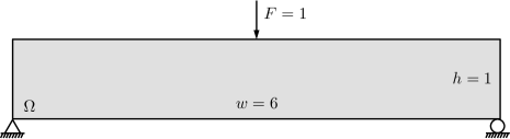
Figure 5: The design domain and boundary conditions for the MBB beam problem

As in the previous algorithm, one can show that $\mathbf{z}_{n}$ is a critical point of $\tilde{J}$ if and only if $\mathbf{z}_{n+1}=\mathbf{z}_{n}$ for all $\tau_{n}>0$. Similarly, if $\mathbf{z}_{n}$ is not a stationary point, then for a sufficiently small step size, the next iterate decreases the value of the cost function, i.e., $\tilde{J}(\mathbf{z}_{n+1})<\tilde{J}(\mathbf{z}_{n})$. The choice of $\tau_{n}$ can be again obtained from an Amijo-type condition along the projection arc (cf. [8]), namely,

$$\tilde{J}(\mathbf{z}_{n})-\tilde{J}(\mathbf{z}_{n+1})\geq\nu\mathbf{d}_{n}^{T}\nabla\tilde{J}(\mathbf{z}_{n})$$ (78)

where the direction vector $\mathbf{d}_{n}$ is given by

$$\left[\mathbf{d}_{n}\right]_{k}=\begin{cases}\left[\mathbf{z}_{n}\right]_{k}-\left[\mathbf{z}_{n+1}\right]_{k}&k\in I_{n}\\ \left[\tau_{n}\mathbf{D}_{n}^{-1}\nabla\tilde{J}(\mathbf{z}_{n})\right]_{k}&k\notin I_{n}\end{cases}$$ (79)

In the next section, we will compare the performance of the forward-backward algorithm consisting of (70) and (71) with the two-metric projection consisting of (75) and (77).

7 Numerical Investigations

The model compliance minimization problem adopted here is the benchmark MBB beam problem, whose domain geometry and prescribed loading and boundary conditions are shown in Figure 5. Using appropriate boundary conditions, the symmetry of the problem is exploited to pose and solve the state equation only on half of the extended domain. The constituent material $\mathbf{C}_{0}$ is assumed to be isotropic with unit Young’s modulus and Poisson ratio of $0.3$. The volume penalty parameter is $\lambda=200/\left|\Omega\right|$ where $\left|\Omega\right|$ is the area of the extended design domain. For all the results in this section, the lower bound on the density is set to $\delta_{\rho}=10^{-3}$ and, unless otherwise stated, the SIMP penalty exponent is fixed at $p=3$. A simple backtracking algorithm is used to determine the value of the step size parameter. Given constants $\tau_{0}>0$ and $0<\sigma<1$, the step size parameter in the $n$th iteration is given by

algorithm	$\mathbf{H}_{n}$	$\tau_{0}$	# it.	# bt.	$\ell(\mathbf{u}_{\rho})$	$R(\rho)$	$V(\rho)$	$\tilde{J}(\rho)$	$E_{1}$	$E_{2}$
FBS	identity	1	316	0	100.019	8.553	0.5120	210.965	9.962e-6	9.943e-5
FBS	identity	2	215	154	100.093	8.537	0.5114	210.914	9.178e-6	5.812e-5
FBS	reciprocal	1	186	0	99.937	8.594	0.5125	211.032	9.769e-6	9.363e-5
FBS	reciprocal	2	91	39	100.095	8.568	0.5117	211.008	4.926e-6	9.746e-5
TMP	identity	1	330	0	100.076	8.533	0.5117	210.951	9.958e-6	9.973e-5
TMP	identity	2	151	78	100.060	8.556	0.5116	210.938	9.639e-6	5.900e-5
TMP	reciprocal	1	179	0	99.943	8.592	0.5125	211.031	9.878e-6	9.453e-5
TMP	reciprocal	2	85	34	100.078	8.578	0.5117	210.999	9.043e-6	8.074e-5

Table 1: Summary of influence of various factors in the algorithm for the MBB problem with $\beta=0.06$. The acronym FBS designates the forward-backward algorithm and TMP refers to the two-metric projection algorithm. Forth and fifth columns show the total number of iterations and backtracking steps. The remaining columns show the final value of compliance $\ell(\mathbf{u}_{\rho})$, regularization term $R(\rho)$, volume fraction $V(\rho)=\left|\Omega\right|^{-1}\int_{\Omega}\rho\mathrm{d}\mathbf{x}$, the regularized objective $\tilde{J}(\rho)$, the relative change in cost function value $E_{1}$ and the error in satisfaction of the first order conditions of optimality $E_{2}$

$$\tau_{n}=\sigma^{k_{n}}\tau_{0}$$ (80)

where $k_{n}$ is the smallest non-negative integer such that $\tau_{n}$ satisfies (69) or (78). In practice, this means that we begin with the initial step size $\tau_{0}$ and reduce it by a factor of $\sigma$ until descent conditions are satisfied. The descent parameter is set to $\nu=10^{-3}$ and the backtracking parameter is $\sigma=0.6$. Note that larger $\nu$ leads to a more severe descent requirement and subsequently smaller $\tau_{n}$. Similarly, smaller $\sigma$ reduces the step size parameter by a larger factor which can decrease the number of backtracking step. Note, however, that using small step sizes may lead to slow convergence of the algorithm.

Since each backtracking step involves evaluating the cost functional and therefore solving the state equation, as a measure of computational cost, we keep track of the total number of backtracking steps (i.e., $\sum_{n}k_{n}$) in addition to the total number of iterations. The convergence criteria adopted here is based on the relative decrease in the objective function

$$E_{1}=\frac{\bigl{|}\tilde{J}(\mathbf{z}_{n+1})-\tilde{J}(\mathbf{z}_{n})\bigr{|}}{\bigl{|}\tilde{J}(\mathbf{z}_{n})\bigr{|}}\leq\epsilon_{1}$$ (81)

and the satisfaction of the first order conditions of optimality according to

$$E_{2}=\frac{\bigl{\|}\mathcal{P}[\mathbf{z}_{n+1}-\nabla\tilde{J}(\mathbf{z}_{n+1})]-\mathbf{z}_{n+1}\bigr{\|}}{\bigl{\|}\mathbf{z}_{n+1}\bigr{\|}}\leq\epsilon_{2}$$ (82)

Here $\mathcal{P}$ is the Euclidian projection onto the constraint set $\left[\delta_{\rho},1\right]^{m}$ defined by $\left[\mathcal{P}(\mathbf{y})\right]_{i}=\min\left(\max\left(0,\left[\mathbf{y}\right]_{i}\right),1\right)$. Unless otherwise stated, we have selected $\epsilon_{1}=10^{-5}$ and $\epsilon_{2}=10^{-4}$.

We begin with the investigation of the behavior of two forms of the algorithm with different choice of parameters discussed in the previous section. In particular, we compare the forward-backward algorithm with the two-metric projection method and investigate the influence of the Hessian approximation. In addition to the choice of $\mathbf{H}_{n}$ defined by (61), we also consider a fixed scaling of the identity matrix

Figure 6: Final density field for the MBB problem and $\beta=0.06$ plotted in grayscale. This result was generated using the TMP algorithm with $\tau_{0}=2$ and $m_{n}=1$

$$\mathbf{H}_{n}\equiv\alpha\mathbf{I},\qquad n=1,2,\dots$$ (83)

for which the algorithm becomes the basic forward-backward algorithm with the same proximal term in every iteration. The scaling coefficient $\alpha$ is set to $4\lambda A$ where $A$ is the area of an element. This choice is made so that the step size parameter $\tau_{n}$ is the same order of magnitude as with reciprocal Hessian. The other parameter investigated here is the initial step size parameter $\tau_{0}$ and we consider two choices $\tau_{0}=1$ and $\tau_{0}=2$. In all cases, the move limit is fixed at $m_{n}=1$ for all $n$ and thus $\mathcal{A}_{n}=\mathcal{A}$.

The model problem is the MBB beam discretized with a grid of 300 by 50 bilinear quad elements and Tikhonov regularization parameter is set to $\beta=0.06$. The initial guess in all cases is taken to be uniform density field $\rho_{h}\equiv 1/2$. All the possible combinations of the above choices produce the same final topology, similar to the representative solution shown in Figure 6. This shows the framework exhibits stable convergence to the same final solution and is relatively insensitive to various choices of algorithmic parameters for this level of regularization. What is different, however, is the speed of convergence and the required computational effort as measured by the number of the backtracking steps, total number of iterations, and cost per iteration. The results are summarized in Table 1.

First we note that the initial step size $\tau_{0}=1$ does not lead to any backtracking steps which means that in each iteration the step size parameter is $\tau_{n}=1$. By contrast, using the larger initial step size parameter $\tau_{0}=2$ requires backtracking steps to satisfy the descent condition but substantially reduces the total number of iterations. Moreover, in all cases, the constant Hessian (83) requires nearly twice as many iterations and backtracking steps compared to the “reciprocal” Hessian. This highlights the fact that embedding the reciprocal approximation of compliance does indeed lead to faster convergence. Overall, the best performance is obtained using the reciprocal approximation and larger initial step size parameter.

For this problem, the forward-backward algorithm and the two-metric projection method roughly have the same number of iterations and backtracking steps. However, the cost per iteration for the two-metric projection is significantly lower since the projection step is computationally trivial. Therefore, the two-metric projection is more efficient.

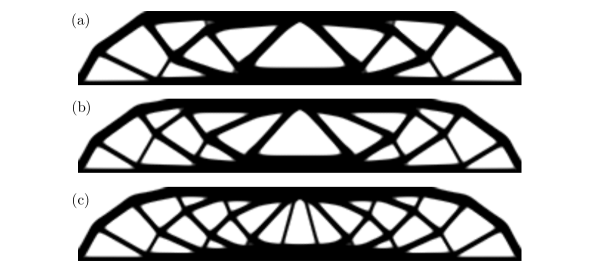
Figure 7: Final densities plotted in grayscale for the MBB problem and $\beta=0.01$. The results are generated using the TMP algorithm with (a) $\tau_{0}=2$, $m_{n}=1$ (b) $\tau_{0}=1$, $m_{n}=1$ (c) $\tau_{0}=1$, $m_{n}=0.03$

Next we investigate the performance of the algorithm for a smaller value of the regularization parameter which is expected to produce more complex topologies. For the next set of results, we set $\beta=0.01$. In all cases considered, the forward-backward and the two-metric projection algorithms both give identical final topologies with roughly the same number of iterations and so we only report the results for the two-metric projection algorithm. Also, as demonstrated by the first study, the use of reciprocal approximation leads to better and faster convergence of the algorithm so we limit the remaining results to the “reciprocal” $\mathbf{H}_{n}$. The tolerance level $\epsilon_{2}=10^{-4}$ for satisfaction of the optimality condition is relatively stringent in this case due to the complexity of final designs (compared to $\beta=0.06$) and leads to a large number of iterations with little change in density near the optimum. We therefore increase the tolerance to $\epsilon_{2}=2\times 10^{-4}$ which gives nearly identical final topologies but with fewer iterations.

We examine the influence of the step size parameter and move limit, which unlike the previous case of large regularization parameter, can lead to different final solutions. We consider two possible initial step size parameters $\tau_{0}=1$ and $\tau_{0}=2$, as well as two choices for the move limit $m_{n}\equiv 1$ and $m_{n}\equiv 0.03$. Here we are using a fixed move limit $m_{n}$ for all iteration $n$. It may be possible to devise a strategy to increase $m_{n}$ in the later stages of optimization to improve convergence. The results are summarized in Table 2 and the final solutions are shown in Figure 7.

First note that with no move limit constraints, i.e., $m_{n}=1$, the final solution with the more aggressive choice of initial step size parameter ($\tau_{0}=2$) is less complex and has fewer members compared to $\tau_{0}=1$, which as before does not require any backtracking steps. Note, however, that the more aggressive scheme in fact requires more iterations to converge. In the presence of move limits, there is no backtracking step with either choice of step size but the larger step size does reduce the total number of iterations. The final topologies are identical and have more members compared to the solutions obtained without the move limits. It is interesting to note that the overall iteration count is lowest for $\tau_{0}=2$ and $m_{n}=0.03$ despite the limit on the change in density in each iteration. As noted earlier, the use of move limits can stabilize the convergence of the topology optimization problem.

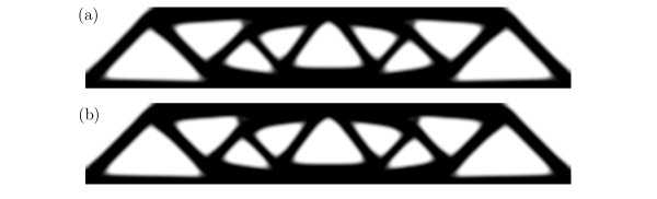
Figure 8: Final densities plotted in grayscale for the MBB problem with $\beta=0.06$ and SIMP penalty exponent (a) $p=4$ (b) $p=5$

The overall trend that the move aggressive choice of parameters produce less complex final solutions is due to the fact that member formation occurs early on in the algorithm. The most aggressive algorithm ($\tau_{0}=2$, $m_{n}=1$) still produces the best solution as measured by $\tilde{J}$ while the solution obtained enforcing the move limit $m_{n}=0.03$ has the lowest value of compliance $J$ (due to distribution of members and slightly higher volume fraction).

We note that aside from the higher degree of complexity, the optimal densities for $\beta=0.01$ contain fewer intermediate values compared to the solution for $\beta=0.06$. One measure of discreteness used in [35] is given by

$$M(\rho)=\frac{1}{\left|\Omega\right|}\int_{\Omega}4\left(\rho-\delta_{\rho}\right)\left(1-\rho\right)\mathrm{d}\mathbf{x}$$ (84)

which is equal to zero if $\rho$ takes only values of $\delta_{\rho}$ and 1. For the solutions shown in Figure 7, $M(\rho)$ is equal to 6.98%, 7.64% and 8.90% from top to bottom, respectively. In contrast, the optimal density for $\beta=0.06$ (cf. Figure 6) has a discreteness measure of 15.0%. By increasing the value of the SIMP exponent $p$, the optimal densities can be made more discrete. The results for $\beta=0.06$ using $p=4$ and $p=5$ are shown in Figure 8. While the optimal topologies are nearly identical to that the solution for $p=3$, the discrete measure is lower to 13.1% and 12.1%, respectively. Observe, however, that the layer of intermediate densities around the boundary cannot be completely eliminated even when $p$ is increase to a very large value since the Tikhonov regularizer is singular in the discontinuous limit of density.

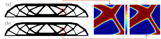
Figure 9: Results of the mesh refinement study with (a) $600\times 100$ (b) $1200\times 200$ elements.

As shown in the previous section, the optimal solutions to the discrete problem converge to an optimal solution of the continuum problem as the finite element mesh is refined. We next demonstrate numerically that solutions produced by the present optimization algorithms appear to be stable with respect to mesh refinement. We do this for the case of $\beta=0.01$ using the two-metric projection algorithm with $\tau_{n}\equiv 1$ where the final topology is relatively complex and the algorithm is expected to be more sensitive. As shown in Figure 9, we solve the problem using finer grids consisting of $600\times 100$ and $1200\times 200$ bilinear square elements. The final density distribution is nearly identical indicating convergence of optimal densities in the $L^{p}$-norm.

Compliant mechanism design

The discussion so far has been limited to the problem of compliance minimization which, as noted earlier, is self-adjoint and its gradient has the same sign. We conclude this section with design of a compliant force inverter for which the cost functional is no longer self-adjoint and therefore, unlike compliance, the gradient field may take both negative and positive values in the domain.

The objective of mechanism design is to identify a structure that maximizes the force exerted on a workpiece under the action of an external actuator. As illustrated in Figure 10, the force inverter transfers the input force of the actuator to a force at the prescribed output location in the opposite direction. We assume in this setting that both the workpiece and the actuator are elastic and their stiffness are represented by vector fields $\mathbf{k}_{1}\in L^{\infty}(\Gamma_{S_{1}})$ and $\mathbf{k}_{2}\in L^{\infty}(\Gamma_{S_{2}})$, respectively. Here $\Gamma_{S_{1}},\Gamma_{S_{2}}$ are segments of the traction boundary $\Gamma_{N}\subseteq\partial\Omega$ where the structure is interacting with these elastic bodies. The tractions experienced by the structure through this interaction for a displacement field $\mathbf{u}$ can be written as

$$\mathbf{t}_{S_{r}}(\mathbf{u})=-\left(\mathbf{k}_{r}\cdot\mathbf{u}\right)\frac{\mathbf{k}_{r}}{\left\|\mathbf{k}_{r}\right\|},\qquad\mbox{on }\Gamma_{S_{r}}\mbox{ for }r=1,2$$ (85)

Accordingly, the displacement $\mathbf{u}_{\rho}$ for a given distribution of material $\rho$ in $\Omega$ is the solution to the following boundary problem

$$a(\mathbf{u}_{\rho},\mathbf{v};\rho)+a_{s}(\mathbf{u}_{\rho},\mathbf{v})=\ell(\mathbf{v})\quad\forall\mathbf{v}\in\mathcal{V}$$ (86)

where

$$a_{s}(\mathbf{u},\mathbf{v})=\sum_{r=1,2}\int_{\Gamma_{S_{r}}}\frac{\left(\mathbf{k}_{r}\cdot\mathbf{u}\right)\left(\mathbf{k}_{r}\cdot\mathbf{v}\right)}{\left\|\mathbf{k}_{r}\right\|}\mathrm{d}s$$ (87)

The cost functional for the mechanism design problem is defined as

$$J(\rho)=-\int_{\Gamma_{S_{1}}}\mathbf{k}_{1}\cdot\mathbf{u}_{\rho}\mathrm{d}s+\lambda\int_{\Omega}\rho\mathrm{d}\mathbf{x}$$ (88)

where the second term again represents a constraint on the volume of the design. The first term of this objective is a measure of the (negative of) force applied to the workpiece in the direction of $\mathbf{k}_{1}$ which can be seen from the following relation:

$$\int_{\Gamma_{S_{1}}}\mathbf{k}_{1}\cdot\mathbf{u}_{\rho}\mathrm{d}s=\int_{\Gamma_{S_{1}}}\left[-\mathbf{t}_{S_{1}}(\mathbf{u}_{\rho})\right]\cdot\frac{\mathbf{k}_{1}}{\left\|\mathbf{k}_{1}\right\|}\mathrm{d}s$$ (89)

Viewed another way, the minimization of the first term of (88) amounts to maximizing the displacement of the structure at the location of the workpiece in the direction of $\mathbf{k}_{1}$.

algorithm	$\tau_{0}$	$m_{n}$	# it.	# bt.	$\ell(\mathbf{u}_{\rho})$	$R(\rho)$	$V(\rho)$	$\tilde{J}(\rho)$	$E_{1}$	$E_{2}$
TMP	1	1	138	0	102.306	4.669	0.4740	201.779	6.989e-6	1.978e-5
TMP	2	1	169	62	102.716	4.075	0.4720	201.189	9.780e-6	1.679e-5
TMP	1	0.03	153	0	100.738	5.185	0.4855	203.014	7.217e-6	1.998e-4
TMP	2	0.03	98	0	100.568	5.173	0.4862	202.970	9.795e-6	1.566e-4

Table 2: Summary of the results for the MBB problem with $\beta=0.01$

The cost functional, in the discrete setting, is given by

$$J(\mathbf{z})=-\mathbf{L}^{T}\mathbf{U}(\mathbf{z})+\lambda\mathbf{z}^{T}\mathbf{v}$$ (90)

where $\left[\mathbf{L}\right]_{i}=\int_{\Gamma_{S_{1}}}\mathbf{k}_{1}\cdot\mathbf{N}_{i}\mathrm{d}s$ and $\mathbf{U}(\mathbf{z})$ solves and, as before, $\mathbf{U}(\mathbf{z})$ is the solution to $\left[\mathbf{K}(\mathbf{z})+\mathbf{K}_{s}\right]\mathbf{U}=\mathbf{F}$. Here $\mathbf{K}_{s}$ is the stiffness matrix associated with bilinear form $a_{s}(\cdot,\cdot)$ and is independent of the design. The gradient of $J$ can be readily computed as $\nabla J(\mathbf{z})=-\mathbf{P}^{T}\overline{\mathbf{E}}(\mathbf{z})+\lambda\mathbf{v}$ where

$$\left[\overline{\mathbf{E}}(\mathbf{z})\right]_{e}=p\left[\mathbf{P}\mathbf{z}\right]_{e}^{p-1}\overline{\mathbf{U}}(\mathbf{z})^{T}\mathbf{k}_{e}\mathbf{U}(\mathbf{z})$$ (91)

and $\overline{\mathbf{U}}(\mathbf{z})$ is the solution to the adjoint problem

$$\left[\mathbf{K}(\mathbf{z})+\mathbf{K}_{s}\right]\overline{\mathbf{U}}=\mathbf{L}$$ (92)

For more details on the formulation of the compliant mechanism design, we refer the reader to [34, 7]. It is evident that $\nabla J$ can take both positive and negative values. The main implication of this for the proposed algorithm is that the reciprocal approximation of the cost functional is not convex and so we cannot use its Hessian directly in the proximal term of the quadratic model. A simple alternative that we tested is to use (61) with the diagonal entries modified as

$$h_{k}(\mathbf{y})=\left|\frac{2}{\left[\mathbf{y}\right]_{k}}\left[\mathbf{P}^{T}\overline{\mathbf{E}}(\mathbf{y})\right]_{k}\right|$$ (93)

Such an approximation has been previously explored by [26, 27] and is similar in spirit to approximations in Svanberg’s Method of Moving Asymptotes [38]. We defer a more detailed study of suitable approximation of the Hessian for general problems to our future work which, as illustrated in this paper, must be based on a priori knowledge of the cost functional.

The compliant mechanism design is known to be more prone to getting trapped in suboptimal local minima. One such local minimum is $\rho_{h}\equiv\delta_{\rho}$ where the entire structure is eliminated and (virtually) no work is transferred between the input actuator and the output location. For this case, the value of the cost functional is roughly zero since there is no density variation and minimum volume of material. To avoid converging to this solution, we use a smaller step size parameter $\tau_{n}=0.1$. Also we begin with small volume penalty parameter of $\lambda=0.02$ which is then increased to $\lambda=0.15$ once the value of cost functional reaches a negative value. This point roughly corresponds to an intermediate density distribution in which the structure connects the input force to the output location. The final solution for $\beta=3\times 10^{-4}$, a grid of $160\times 160$ quadrilateral elements, and the two-metric projection algorithm is shown in Figure 10. This solution required a total of 140 iterations.

8 Discussion and Concluding Remarks

Since the splitting algorithm presented here is a first-order method, it is also appropriate to compare its performance to the gradient projection algorithm, which is among the most basic first-order methods for solving constrained optimization problems. The next iterate in the gradient projection method is simply the projection of the unconstrained gradient descent step onto the admissible space. In the absence of move limits and in the discrete setting, we have the following update expression

$$\mathbf{z}_{n+1}=\underset{\mathbf{z}\in\left[\delta_{\rho},1\right]^{m}}{\mbox{argmin}}\ \left\|\mathbf{z}-\left[\mathbf{z}_{n}-\frac{\tau_{n}}{\alpha}\nabla\tilde{J}(\mathbf{z}_{n})\right]\right\|^{2}$$ (94)

where the scaling parameter $\alpha=4\lambda A$ is defined as before in order to allow for a direct comparison with the forward-backward splitting in the case $\mathbf{H}_{n}=\alpha\mathbf{I}$. We determine the step size parameter $\tau_{n}$ in each iteration using the backtracking procedure (80) based on the Armijo-type descent condition (69). Note that due to the simple structure of the constraint set, computing the gradient $\nabla\tilde{J}$ constitutes the main computational cost of the gradient projection algorithm in each iteration. Table 3 summarizes the results for the MBB beam problem with $\beta=0.06$ for two different choice of initial step size parameter $\tau_{0}$. First observe that the step sizes are smaller compared to the forward-backward algorithm, a fact that can be seen from the equivalent expression for (94) given by

$$\mathbf{z}_{n+1}=\underset{\mathbf{z}\in\left[\delta_{\rho},1\right]^{m}}{\mbox{argmin}}\ \tilde{J}(\mathbf{z}_{n})+\left(\mathbf{z}-\mathbf{z}_{n}\right)^{T}\nabla\tilde{J}(\mathbf{z}_{n})+\frac{1}{2\tau_{n}}\left\|\mathbf{z}-\mathbf{z}_{n}\right\|_{\alpha\mathbf{I}}^{2}$$ (95)

This shows that in each iteration, we construct a quadratic model for the composite objective $\tilde{J}$. By constrast, the quadratic model in (58) is only used for $J$ and the regularization term appears exactly. Since $\nabla\tilde{J}$ has a larger Lipschitz constant compared to $\nabla J$, it is therefore expected that $\tau_{n}$ must be smaller to ensure descent. It is also instructive to recall the informal derivation of the forward-backward algorithm in [41] where the main difference with the gradient projection algorithm was the use of a semi-implicit (in place of an explicit) temporal discertization of the gradient flow equation. Note that the gradient projection algorithm converged to the same solution as before (cf. Figure 6) though in the case of $\tau_{0}=0.25$, the convergence was too slow and we terminated the algorithm after 1,000 iterations.

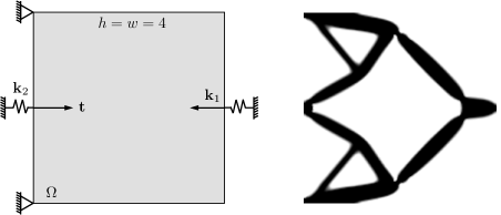
Figure 10: The design domain and boundary conditions for the force inverter problem (left) and the optimal topology (right). For this example, $\left\|\mathbf{k}_{1}\right\|=\left\|\mathbf{k}_{2}\right\|=0.1$

Since the Method of Moving Asymptotes [38] is the most widely used algorithm in the topology optimization literature, we also tested its performance using the same MBB problem. We followed the common practice and used the algorithm as a black-box optimization routine. In particular, we provided the algorithm with the gradient of composite objective $\tilde{J}$ and did not make any changes to the open source code provided by Svangberg. MMA internally generates a separable convex approximation to $\tilde{J}$ using reciprocal-type expansions with appropriately defined and updated asymptotes. Though such approximations are suitable for the structural term, they may be inaccurate for the Tikhonov regularizer and the composite objective. As shown in Table 3, MMA did not converge (according to the convergence criteria described earlier) in 1,000 iterations before it was terminated. Furthermore, not only was the final value of the objective function larger than that obtained by gradient projection or either splitting algorithm, the final density was topologically different from the solution shown in the Figure 6.

The fact that the present splitting framework outperforms MMA should not be surprising. Unlike MMA, which is far more general and can handle a much broader class of problems [39], the present algorithm is tailored to the specific structure of (6) (or (52) in the discrete setting) and provides an ideal treatment of its constituents. First, the composite objective is the sum of two terms and algorithm deals with each term separately. The regularization term $R$ is represented with a high degree fidelity since the resulting subproblem with its simple structure can be solved efficiently. The structural term $J$, while expensive to compute, contains many local minima and very fast convergence usually at best reaches a suboptimal local minimum. Moreover, $J$ tends to be rather flat near stationary points and so one should not require a high level accuracy for satisfaction of the first order conditions of optimality. As a side remark, these characteristics indicate that second order methods do not pay off given their significantly higher computational cost per iteration. The other drawback of using exact second order information is the storage requirements, quadratic in the size of the problem, which can be prohibitive for large-scale problems such as those encountered in practical applications of topology optimization. Therefore, first order methods are better suited for minimizing $J$.

In the splitting algorithm proposed here, we use additional knowledge about the behavior of $J$ to construct accurate approximations using only first order information and minimal storage requirements. Furthermore, the two-metric approach allows for a computationally efficient treatment of the constraint set. In fact, the proposed approach is aligned with the renewed interest in first-order convex optimization algorithms for solving large-scale inverse problems in signal recovery, statistical estimation, and machine learning [44, 21, 14, 22]. Our rather restricted and narrow comparison with MMA is meant to motivate the virtue of developing such tailored algorithms. We note that, aside from efficiency, robustness is also a major issue for solving topology optimization problems (see, for example, comments in [10] on total variation regularization). Although the high sensitivity to parameters is, to a large extent, intrinsic to the size, nonconvexity and sometimes nonsmoothness of these problems, we emphasize that it should be minimized as much as possible. Developing an appropriately-designed optimization algorithm that fits the structure of the problem at hand can be key to achieving this.

algorithm	$\tau_{0}$	# it.	# bt.	$\tilde{J}(\rho)$	$E_{2}$
GP	0.25	1000*	0	210.74	1.362e-4
GP	0.5	568	79	210.68	8.939e-5
MMA	–	1000*	0	213.39	1.913e-4

Table 3: Summary of the results for gradient projection and MMA algorithm for the MBB beam problem with $\beta=0.06$. The asterisk indicates that the maximum allowed iteration count of 1,000 was reached before the convergence criteria was met

In the extensions of this work, we intend to consider nonsmooth regularizers such as the total variation of density within the present variable metric scheme. This would require the extension of available denoising algorithms (e.g. [18, 14]) for solving the resulting subproblems in each iteration. Also of interest is the use of accelerated first order methods such as those proposed in [28] and [4] that can improve the convergence speed of the algorithms. Developing a two-metric variation of such algorithms for the constrained minimization problems of topology optimization is promising.

References

- [1] M. Adlers, Sparse Least Squares Problems with Box Constraints, Department of Mathematics, Linkoping University, Thesis, 1998.
- [2] G. Allaire, Shape Optimization by the Homogenization Method, Springer, New York, 2001.
- [3] J. S. Arora, Analysis of optimality criteria and gradient projection methods for optimal structural design, Comput Methods Appl Mech Engrg, 23 (1980), pp. 185–213.
- [4] A. Beck and M. Teboulle, A fast iterative shrinkage-thresholding algorithm for linear inverse problems, SIAM J Image Sci, 2 (2008), pp. 183–202.
- [5] , Gradient-based algorithms with applications to signal recovery problems, in Convex Optimization in Signal Processing and Communications, Cambridge university press, 2010.
- [6] M. P. Bendsøe, Optimal design as material distribution probelm, Struct Optimization, 1 (1989), pp. 193–202.
- [7] M. P. Bendsøe and O. Sigmund, Topology Optimization: Theory, Methods and Applications, Springer, 2003.
- [8] D. P. Bertsekas, Projected newton methods for optimization problems with simple constraints, SIAM J Control Opt, 20 (1982), pp. 221–246.
- [9] , Nonlinear Programming, Athena Scientific, 2nd ed., 1999.
- [10] T. Borrvall, Topology optimization of elastic continua using restriction, Arch Comput Method E, 8 (2001), pp. 251–285.
- [11] T. Borrvall and J. Petersson, Topology optimization using regularized intermediate density control, Comput Methods Appl Mech Engrg, 190 (2001), pp. 4911–4928.
- [12] B. Bourdin, Filters in topology optimization, Int J Numer Meth Eng, 50 (2001), pp. 2143–2158.
- [13] B. Bourdin and A. Chambolle, Design-dependent loads in topology optimization, ESAIM Contr Optim Ca, 9 (2003), pp. 19–48.
- [14] K. Bredies, A forward–backward splitting algorithm for the minimization of non-smooth convex functionals in Banach space, Inverse Probl, 25 (2009), p. 015005.
- [15] S. C. Brenner and L. R. Scott, The Mathematical Theory of Finite Element Methods, Springer, 2nd ed., 2002.
- [16] T. Bruns and D. A. Tortorelli, Topology optimization of non-linear elastic structures and compliant mechanisms, Comput Methods Appl Mech Engrg, 190 (2001), pp. 3443–3459.
- [17] M. Burger and R. Stainko, Phase-field relaxation of topology optimization with local stress constraints, SIAM J Control Optim, 45 (2006), pp. 1447–1466.
- [18] A. Chambolle, An algorithm for total variation minimization and applications, J Math Imaging Vis, 20 (2004), pp. 89–97.
- [19] G. H. G. Chen and R. T. Rockafellar, Convergence rates in forward-backward splitting, SIAM J Optimiz, 7 (1997), pp. 421–444.
- [20] G. Cohen, Optimization by decomposition and coordination: a unified approach, IEEE Trans Autom Control, 23 (1978), pp. 222–232.
- [21] P. L. Combettes and V. R. Wajs, Signal recovery by proximal forward-backward splitting, Multiscale Model Sim, 4 (2006), pp. 1168–1200.
- [22] J. Duchi and Y. Singer, Efficient online and batch learning using forward backward splitting, J Mach Learn Res, 10 (2009), pp. 2899–2934.
- [23] L. C. Evans, Partial Differential Equations, Graduate Studies in Mathematics, American Mathematical Society, Rhode Island, 1998.
- [24] E. M. Gafni and D. Bertsekas, Two-metric projection methods for constrained optimization, SIAM J Control Opt, 20 (1984), pp. 936–964.
- [25] A. A. Groenwold and L. F. P. Etman, On the equivalence of optimality criterion and sequential approximate optimization methods in the classical topology layout problem, Int J Numer Meth Eng, 73 (2008), pp. 297–316.
- [26] , A quadratic approximation for structural topology optimization, Int J Numer Meth Eng, 82 (2010), pp. 505–524.
- [27] A. A. Groenwold, L. F. P. Etman, and D. W. Wood, Approximated approximations for SAO, Struct Multidisc Optim, 41 (2010), pp. 39–56.
- [28] Y. Nesterov, Gradient methods for minimizing composite objective function. available at http://www.ecore.be/DPs/dp1191313936.pdf., 2007.
- [29] M. Patriksson, Cost approximation: A unified framework of descent algorithms for nonlinear programs, SIAM J Optimiz, 8 (1998), pp. 561–582.
- [30] J. Petersson, Some convergence results in perimeter-controlled topology optimization, Comput Methods Appl Mech Engrg, 171 (1999), pp. 123–140.
- [31] J. Petersson and O. Sigmund, Slope constrained topology optimization, Int. J. Numer. Meth. Engng, 41 (1998), pp. 1417–1434.
- [32] G. I. N. Rozvany, A critical review of established methods of structural topology optimization, Struct Multidisc Optim, 37 (2009), pp. 217–237.
- [33] G. I. N. Rozvany, M. Zhou, and T. Birker, Generalized shape optimization without homogenization, Struct Optimization, 4 (1992), pp. 250–252.
- [34] O. Sigmund, On the design of compliant mechanisms using topology optimization, Mechanics Based Design of Structures and Machines, 25 (1997), pp. 493–524.
- [35] , Morphology-based black and white filters for topology optimization, Struct Multidisc Optim, 33 (2007), pp. 401–424.
- [36] O. Sigmund and K. Maute, Sensitivity filtering from a continuum mechanics perspective, Struct Multidisc Optim, 46 (2012), pp. 471–475.
- [37] O. Sigmund and J. Petersson, Numerical instabilities in topology optimization: A survey on procedures dealing with checkerboards, mesh-dependencies and local minima, Struct Optimization, 16 (1998), pp. 68–75.
- [38] K. Svanberg, The Method of Moving Asymptotes–A new method for structural optimization, Int J Numer Meth Eng, 24 (1987), pp. 359–373.
- [39] , A class of globally convergent optimization methods based on conservative convex separable approximations, SIAM J Optimiz, 12 (2001), pp. 555–573.
- [40] A. Takezawa, S. Nishiwaki, and M. Kitamura, Shape and topology optimization based on the phase field method and sensitivity analysis, J Comput Phys, 229 (2010), pp. 2697–2718.
- [41] C. Talischi and G. H. Paulino, An operator splitting algorithm for Tikhonov-regularized topology optimization, Comput Methods Appl Mech Engrg, 253 (2013), pp. 599–608.
- [42] C. Talischi, G. H. Paulino, A. Pereira, and I. F. M. Menezes, Polygonal finite elements for topology optimization: A unifying paradigm, Int J Numer Meth Eng, 82 (2010), pp. 671–698.
- [43] , PolyTop: a Matlab implementation of a general topology optimization framework using unstructured polygonal finite element meshes, Struct Multidisc Optim, 45 (2012), pp. 329–357.
- [44] S. J. Wright, Optimization in machine learning, in Neural Information Processing Systems (NIPS) Workshop, 2008.