The statistical nature of the brightest group galaxies

Abstract

We examine the statistical properties of the brightest group galaxies (BGGs) using a complete spectroscopic sample of groups/clusters of galaxies selected from the Data Release 7 of the Sloan Digital Sky Survey. We test whether BGGs and other bright members of groups are consistent with an ordered population among the total population of group galaxies. We find that the luminosity distributions of BGGs do not follow the predictions from the order statistics (OS). The average luminosities of BGGs are systematically brighter than OS predictions. On the other hand, by properly taking into account the brightening effect of the BGGs, the luminosity distributions of the second brightest galaxies are in excellent agreement with the expectations of OS. The brightening of BGGs relative to the OS expectation is consistent with a scenario that the BGGs on average have over-grown about 20 percent masses relative to the other member galaxies. The growth ($\Delta M$) is not stochastic but correlated with the magnitude gap ($G_{1,2}$) between the brightest and the second brightest galaxy. The growth ($\Delta M$) is larger for the groups having more prominent BGGs (larger $G_{1,2}$) and averagely contributes about 30 percent of the final $G_{1,2}$ of the groups of galaxies.

1. INTRODUCTION

The brightest group/cluster galaxies (hereafter BGGs) are typically red, old ellipticals located near the centers of their dark matter host haloes. Because of their extreme brightness and uniformity in luminosity, they can be used to trace the large scale structure and to study galaxy evolution in massive haloes (Postman & Lauer, 1995; Rozo et al., 2010; Ascaso et al., 2011; Wen & Han, 2011). On the other hand, BGGs are also known to differ from ordinary ellipticals in their more extended surface brightness profiles and in their deviations from scaling relations obeyed by other ellipticals (e.g., Bernardi et al., 2007; von der Linden et al., 2007; Liu et al., 2008).

In the framework of hierarchical structure formation in a $\Lambda$CDM cosmology, galaxies build up their stellar mass through mergers with other galaxies, and through in-situ star formation, fed by cold flows and/or cooling flows that deliver gas to the potential well centers of their host haloes. In the absence of any environmental effects, BGGs should simply be statistical extremes: their extreme luminosities/stellar masses are merely a consequence of them being defined as the brightest/most massive galaxies in their group. Put differently, from a physical point of view, there is nothing special about a BGG. However, it is well known that environment does play an important role. Of particular importance is the distinction between central galaxies, defined as the galaxy in a host halo with the minimal specific potential energy, and satellite galaxies, which are galaxies that orbit around a central galaxy (see e.g. van den Bosch et al., 2008; Weinmann et al., 2009; Pasquali et al., 2010). Typically central galaxies are expected to grow in mass by cannibalizing their satellites (Dubinski, 1998; Cooray & Milosavljević, 2005) and by being the repositories of cooling flows [although AGN feedback may prevent such gas from being turned into stars; e.g. Rafferty et al. (2008)], whereas satellite galaxies are subjected to a number of processes that quench star formation (i.e., ram-pressure stripping, strangulation) and strip mass (i.e. tidal stripping). If these ‘environmental’ effects have a significant impact on the luminosities and/or stellar masses of the galaxies, one might expect BGGs, which typically are central galaxies (though not always, see e.g. Skibba et al., 2011) to evolve into a distinct population.

There are still controversies concerning the statistical nature of BGGs. Early analysis (Peebles, 1968; Geller & Peebles, 1976; Geller & Postman, 1983) found that the luminosity distribution of BGGs is consistent with an statistical extreme value population. More recent analyses, using statistical tests such as the asymptotic form of the BGG luminosity function (Bhavsar & Barrow, 1985) and the luminosity gap between the first and second ranked group members (Tremaine & Richstone, 1977; Loh & Strauss, 2006; Lin et al., 2010; Tavasoli et al., 2011), reached the opposite conclusion: BGGs are distinct compared to the extreme value statistics (however, see Paranjape & Sheth (2012). There have also been investigations that attempt to reconcile the two results by considering two populations for the BGGs (Bhavsar, 1989; Bernstein & Bhavsar, 2001). Most of these analysis focused on rich clusters, where the number of member galaxies is large but the total number of systems is limited. More recently, Dobos & Csabai (2011) applied an order statistics to a large sample of luminous red galaxies (LRG) selected from the Sloan Digital Sky Survey (SDSS, York, 2000) Data Release 7 (DR7, Abazajian, 2009) and concluded that LRGs can be viewed as an extreme value sample when they are binned in redshift rather than in terms of the richness of their host group. Using LRGs selected from the SDSS and the SDSS-III Baryon Oscillation Spectroscopic Survey (Schlegel et al., 2009), Tal et al. (2012) found that the large luminosity gap between the LRG and the most luminous satellite can be reproduced by sparsely sampling a Schechter function obtained for galaxies in random fields, suggesting that LRGs obey extreme value statistics(see also More, 2012; Paranjape & Sheth, 2012; Hearin et al., 2013b).

In the present paper, we study the statistical properties of BGGs using an order statistics analysis similar to that carried out by Dobos & Csabai (2011). The order statistics (hereafter OS) studies the expected distribution of the $k$-th order (largest value) of a given quantity (e.g. luminosity) among a sample (group) with $N$ members (galaxies) which are randomly drawn from an underlying probability density distribution. The extreme value statistic (hereafter EVS) thus corresponds to $k=1$ of the OS. Our analysis is based on galaxies in individual groups selected from a large spectroscopic survey, the SDSS DR7. This allows us to divide our group sample into different richness bins, and to study the luminosity distribution of the member galaxies separately for each of the richness bins (Section 2). We simulate statistical samples by building mock groups using the observed group member distribution function, and compare the properties of the member galaxies in a given rank between real and simulated samples to examine whether the luminosity distributions of BGGs and other highly-ranked member galaxies are consistent with the OS populations (Section 3). Simple models are then presented to understand how BGGs may over-grow their masses relative to other members (Section 4). The specialties of BGGs are further discussed in Section 5 using the Tremaine-Richestone test(Tremaine & Richstone, 1977) . Finally we summarize our results and make discussions in Section 6.

2. The Data

In this paper, we use the SDSS galaxy group catalogs of Yang et al. (2007), constructed using the adaptive halo-based group finder of Yang et al. (2005). The groups are selected from the DR7 version of the New York University Value-Added Galaxy Catalogue (NYU-VAGC, Blanton et al., 2005). From NYU-VAGC, we select all galaxies in the Main Galaxy Sample with redshifts in the range $0.01\leq z\leq 0.20$ and with a redshift completeness $c>0.7$. The resulting SDSS galaxy catalog contains a total of $639,359$ galaxies, with a sky coverage of 7,748 square degrees.

Because of the fiber collision effect in the SDSS observation, two fibers on the same plate cannot be closer than 55 arcsecs and so a small fraction of galaxies (about 7 percent) eligible for spectroscopy do not have spectroscopic measurements. As a result, three group catalogs are provided in Yang et al. (2007), samples I, II and III. Sample I only includes the galaxies with measured redshifts from the SDSS, whereas sample II are further supplied with a small fraction of galaxies with spectroscopic redshifts from other redshift catalogs. In Sample III, those galaxies without spectroscopic measurements are assigned redshifts according to their nearest neighbors. To avoid incompleteness, we use sample III as our group catalog. As pointed out in Yang et al. (2007), the added redshifts in sample III may cause the number of members of some of the galaxy groups to be overestimated. However, since we are mainly concerned with the brightest galaxies, this fiber-collision effect is not expected to have a significant impact on our results. Indeed, we have tested that using sample II leads to negligible changes in all of our conclusions.

For each group in the catalog, the model magnitudes are used for both luminosity and stellar mass measurements. A characteristic luminosity $L_{19.5}$ and a characteristic stellar mass $M_{19.5}$ are defined, respectively, as the total luminosity and total stellar mass of all group members with $M_{\rm r}<-19.5$. The $r$ band absolute magnitude $M_{\rm r}$ is calculated from the SDSS galaxy model magnitude and $K+E$ corrected to redshift $z=0.1$. The host halo mass of each group is then estimated using the abundance matching of $L_{19.5}$ or $M_{19.5}$ with the halo mass according to the halo mass function given by Tinker et al. (2008) for spherical over-density $\Delta=200$. The cosmological parameters used for the halo mass function are consistent with the 7-year data release of the WMAP mission: $\Omega_{\rm m}=0.275$, $\Omega_{\rm\Lambda}=0.725$, $h=0.702$, and $\sigma_{8}=0.816$ (Komatsu et al., 2011), where the reduced Hubble constant, $h$, is defined through the Hubble constant as $H_{0}=100h~{}{\rm km~{}s^{-1}~{}Mpc^{-1}}$.

The halo masses for the galaxy groups described above are cosmology and model dependent. To reduce such dependence, we use instead a richness parameter $N_{\rm 19.5}$, defined as the number of member galaxies with $M_{\rm r}<-19.5$, as a halo-mass proxy. As we will show, this richness parameter also plays as a key parameter in the OS study. Since group members are identified from the SDSS spectroscopic galaxy catalog, which is complete to $r\sim 17.77$, $N_{\rm 19.5}$ can be obtained for all the groups at redshift $z<0.09$. For our analysis, we use only groups with $z<0.09$, which therefore is a volume complete sample. We exclude the groups with all their members fainter than $-19.5$ mag. Such groups have no halo mass been estimated in Yang et al. (2007) and have $N_{\rm 19.5}=0$ in our definition. We also eliminate all groups with $f_{\rm edge}<0.9$ to reduce boundary effects, where $f_{\rm edge}$ is a measure for the volume of the group that lies within the SDSS survey edges(see Yang et al. 2007 for details). The total number of finally selected groups is 113,436 and the number of member galaxies with $M_{\rm r}<-19.5$ is 159,503.

We show the distributions of some of the basic parameters of our group sample in Fig. 1. The top left panel shows the histograms of group richness $N_{\rm 19.5}$. Our group sample includes a large population that only having one group member, i.e. $N_{\rm 19.5}=1$. These single galaxies are the cases that no any other bright members can be found inside their linking radii. In other words, all of their satellites were fainter than $-19.5$ mag. The number of such $N_{\rm 19.5}=1$ groups is 97,422. Besides them, our group sample spans a very wide range, from poor groups ($N_{\rm 19.5}=2$) to rich clusters ($N_{\rm 19.5}>100$). The richest cluster in our sample has $N_{\rm 19.5}=144$ (Abell 2029). For $N_{\rm 19.5}\geq 2$ groups, the host halo mass($M_{\rm h}$) ranges from $10^{12}h^{-1}M_{\odot}$ to $\sim 10^{14.5}h^{-1}M_{\odot}$. Their $M_{\rm h}$ distribution is shown as the solid histogram in the top right panel of 1. In this panel, we also plot the $M_{\rm h}$ distribution of the single galaxies($N_{\rm 19.5}=1$) as a separated dotted histogram. As we can see, the $M_{\rm h}$ of single galaxies also has a wide distribution, about two orders of magnitude from $10^{11.6}h^{-1}M_{\odot}$ to $\sim 10^{13.5}h^{-1}M_{\odot}$. This wide $M_{\rm h}$ distribution of single galaxies stems from their wide luminosity distribution, which is shown as the dotted histogram in the bottom left panel of Fig. 1. In that panel, we also show the BGG magnitude($M_{1}$) distribution of the $N_{\rm 19.5}\geq 2$ groups as the solid histogram for comparison. The luminosity distribution of the single galaxies has a monotonic shape, which can be approximated with a Schechter function. On the other hand, the$M_{1}$ distribution of the $N_{\rm 19.5}\geq 2$ groups shows a peaks at $M_{\rm r}\sim-21.7$ and has a very wide dispersion, spanning from our sample limit $M_{\rm r}=-19.5$ to the very bright end $\sim-23.3$. As we will show in next sections, both of the peak and dispersion of the BGG magnitudes are actually functions of $N_{\rm 19.5}$. The bottom right panel shows the distribution of $G_{1,2}$, the magnitude gap between the BGG and the second brightest group galaxy,

$$G_{1,2}=M_{2}-M_{1}\,.$$ (1)

This quantity plays an important role in the test of the statistical properties of the BGGs (see Sections 4.3 and Section 5).

Figure 1.— The number histograms of the richness $N_{\rm 19.5}$, halo mass $M_{\rm h}$, BGG absolute magnitude $M_{1}$ and magnitude gap $G_{1,2}$ of our group sample. In the $M_{\rm h}$ and $M_{1}$ panels, the histograms of the single galaxies($N_{\rm 19.5}=1$) and groups($N_{\rm 19.5}\geq 2$) are shown by the dotted and solid histograms separately.

2.1. The $M_{\rm h}$-$N_{\rm 19.5}$ correlation

The halo mass ($M_{\rm h}$) we used is obtained by matching the number density of groups with the characteristic luminosity(the total luminosities of the $M_{\rm r}<-19.5$ group members) above $L_{19.5}$ with the number density of dark matter haloes with masses above $M_{\rm h}$ predicted by a halo mass function (Yang et al., 2007). Not surprisingly, a strong correlation between the group richness $N_{\rm 19.5}$ and $M_{\rm h}$ is expected.

We show the correlation between $N_{\rm 19.5}$ and $M_{\rm h}$ in Fig. 2, where the stars show the mean halo masses (in logarithm space) at each $N_{\rm 19.5}$. In this plot, we see again that $M_{\rm h}$ has a very large variance for single galaxies($N_{\rm 19.5}=1$). With the increasing of $N_{\rm 19.5}$, the variance of $M_{\rm h}$ at given $N_{\rm 19.5}$ decreases systematically. This is because the variance of $L_{19.5}$(so that $M_{\rm h}$) decreases with the increasing of $N_{\rm 19.5}$ for any given conditional luminosity function of the group members. The mean $\log M_{\rm h}$ shows a linear correlation with $\log N_{\rm 19.5}$ for rich groups with $N_{\rm 19.5}\geq 7$. Such a linear relation has also been obtained in other studies where the halo masses are estimated from independent measurements, e.g., satellite kinematics (Becker et al., 2007) and the X-ray data (Andreon & Hurn, 2010). For poor groups with $N_{\rm 19.5}<7$, however, the slope of the $M_{\rm h}$ - $N_{\rm 19.5}$ relation becomes steeper, which is attributed to the different shapes between the halo mass function and group member luminosity function at the low mass end. For simplicity, we fit the $M_{\rm h}$-$N_{\rm 19.5}$ correlation with a broken-power law which breaks at $N_{\rm 19.5}=7$. Fixing the power law index to be $n=1$ at $N_{\rm 19.5}\geq 7$ we find that

$$M_{\rm h}=\left\{\begin{array}[]{ll}10^{12.04}\,N_{\rm 19.5}^{1.90}\,h^{-1}M_{\odot}&\mbox{if $N_{\rm 19.5}<7$}\\ 10^{12.72}\,N_{\rm 19.5}\,h^{-1}M_{\odot}&\mbox{if $N_{\rm 19.5}\geq 7$}\end{array}\right.\,.$$ (2)

This is shown in Fig. 2 as the solid line. The scatter in the relation is quite small for rich systems (about 0.2 dex at $N_{\rm 19.5}=7$), so that $N_{\rm 19.5}$ is a good indicator of halo mass. For poorer systems, the scatter becomes increasingly larger. Because it has been assumed that there is no scatter between $L_{19.5}$ and $M_{\rm h}$(Yang et al., 2007), the scatter of $M_{\rm h}$ at given $N_{\rm 19.5}$ actually reflects the scatter between $L_{19.5}$ and $N_{\rm 19.5}$.

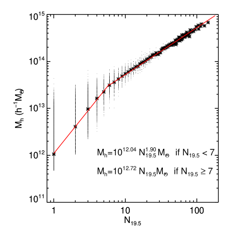
Figure 2.— The correlation between the group richness $N_{\rm 19.5}$ and the host halo mass $M_{\rm h}$. The solid line shows the fitting relation of Equ. (2)

Although $N_{\rm 19.5}$ and $M_{\rm h}$ have a correlation as shown in Equ. 2, they are two different measurements of the global properties of groups. From statistical point of view, our sample is complete in $N_{\rm 19.5}\geq 1$ while it is not in $M_{\rm h}\geq M_{\rm h,min}$, where $M_{\rm h,min}$ is the minimum $M_{\rm h}$ of our group sample, $\sim 5\times 10^{11}h^{-1}M_{\odot}$. The reason is that there is no $M_{\rm h}$ estimation for these groups with all their members fainter than $-19.5$ mag(i.e. $N_{\rm 19.5}=0$). In our group sample, $M_{\rm h,min}$ corresponds to the case of a single galaxy with the minimal sample luminosity $M_{\rm r}=-19.5$ mag. It is certain that there are $N_{\rm 19.5}=0$ groups with $M_{\rm h}\geq M_{\rm h,min}$. Therefore, in following, we will use $N_{\rm 19.5}$ as the reference parameter of the groups to make OS studies. When required, we will use Equ. 2 to make discussions on $M_{\rm h}$.

2.2. Group member luminosity function

To quantify the statistical nature of BGGs, the luminosity distribution of the group members need to be determined. The group member luminosity function is shown to depend on the host halo mass (Hansen et al., 2005; Weinmann et al., 2006; Yang et al., 2008; Hansen et al., 2009). Here, we present the luminosity distributions of the group members in different richness bins.

For $N_{\rm 19.5}=1$ groups, the group member luminosity distribution equals to the BGG luminosity distribution and we can not obtain any further conclusions from OS. Therefore, we will limit our following studies only on $N_{\rm 19.5}\geq 2$ groups. For clarity, we will note $N_{\rm 19.5}=1$ groups as ‘single galaxies’ hereafter. When we state ‘group’, we only refer to the groups with $N_{\rm 19.5}\geq 2$.

We separate our groups into 6 $N_{\rm 19.5}$ bins: $[2,2]$, $[3,4]$, $[5,6]$, $[7,10]$, $[11,20]$, $[21,144]$. The widths of the bins are a compromise between the resolution in $N_{\rm 19.5}$ and the number of groups and group members within each bin. For reference, the average logarithmic halo mass, the number of groups and group members are listed in Table 1 for each of the richness bins.

The conditional luminosity functions (hereafter CLF) of the group members in different richness bins are shown as the solid histograms in Fig. 3. To see whether the CLF changes with group richness(halo mass), we also plot in each panel the luminosity function of the single galaxies as a reference(dashed line). In a given panel, this function has been normalized by the same number of the group members in each $N_{\rm 19.5}$ bin. As we can see, the CLFs of the group members in all $N_{\rm 19.5}$ bins are brighter than the luminosity function of the single galaxies and vary significantly with $N_{\rm 19.5}$. Groups with increasing $N_{\rm 19.5}$ contain systematically larger fraction of bright galaxies with $M_{\rm r}<-22$. The Kolmogorov-Smirnov (KS) test probabilities that the CLFs follow the same distribution are close to zero for any two $N_{\rm 19.5}$ bins.

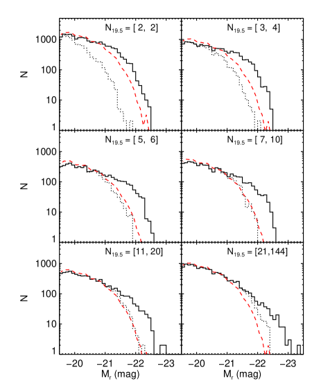
Figure 3.— The $r$ band absolute magnitude distributions of the group members(solid histograms) and the satellites(dotted histograms) in different $N_{\rm 19.5}$ bins. In each panel, the dashed line shows the luminosity distribution function of the single galaxies, which are normalized to the same number of the group members in each $N_{\rm 19.5}$ bin.

In each panel of Fig. 3, we also show the CLF of the satellite members, i.e. the $M_{\rm r}$ distribution of the group members except BGGs, as the dotted histogram. Similar as the CLFs of all group members, the satellite distribution functions also show a systematical dependence on $N_{\rm 19.5}$. Satellites are also on average brighter in higher mass haloes.

In OS, the statistical properties of the $k$th order ($k$th brightest) members depend both on the sample size $N$ ($N_{\rm 19.5}$ in our case) and the underlying distribution function of the sample members (Dobos & Csabai, 2011; Paranjape & Sheth, 2012). In Fig. 3, we have shown that the CLFs of the group members and the CLFs of the satellites both vary systematically with the group richness (halo mass). This demonstrates clearly that galaxies in these groups do not have the underlying luminosity distribution as the general population. This also means that BGGs cannot be tested as the extremes of a general galaxy population. Paranjape & Sheth (2012) showed that the group members follow a universal luminosity distribution. However, their conclusions are only based on the comparison between two subsamples of groups with $N\geq 10$ and $N\geq 15$ members.

Thus, in our following study of the statistical properties of the group members using OS, we will consider groups in given $N_{\rm 19.5}$ bins, and use the CLF corresponding to the $N_{\rm 19.5}$ as the underlying distribution to test if BGGs are consistent with the extreme value statistics of the galaxy population contained in such groups.

3. The order statistic prediction

In this section, we start from the observed CLFs and make predictions for the statistical properties of the BGGs and other bright members using OS. By comparing the statistical properties of the ordered members of the real groups with the OS predictions, we test whether BGGs and other bright members are consistent with the OS.

3.1. The brightest group galaxies

We make OS predictions for BGGs by building a sample of mock groups for each $N_{\rm 19.5}$ bin, which is designed to have the same richness distribution and underlying luminosity distribution as the real groups but with their members assigned in a statistical (random) way. To achieve this, we make mock groups that have exactly the same richness as the real groups in the sample. We then assign random luminosities to the members of each mock according to the observed CLF (solid histogram in Fig. 3). By this construction, the BGGs of the mock groups can be compared with the BGGs of the real groups. For clarity, we refer to the mock groups as OS groups, and the BGGs of the OS groups as OS BGGs.

We show the histograms of the absolute magnitude of the real and OS BGGs in Fig. 4. In each panel ($N_{\rm 19.5}$ bin), the solid histogram shows the real BGGs, while the dotted histogram represent the OS BGGs. We make a comparison of the $M_{1}$ distributions of the real BGGs and OS BGGs with a non-parametric KS test. The KS test probability that the real BGGs follow the same distribution as the OS BGGs ($P_{\rm OS}$) is labeled on top of each panel. As we can see, for all richness bins, the KS test probabilities that the OS BGGs follow the same distributions as the real BGGs are very small ($<10^{-4}$).

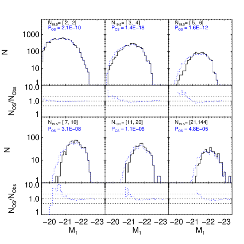
Figure 4.— The distributions of the $r$ band absolute magnitudes of the BGGs in six $N_{\rm 19.5}$ bins (as indicated in each of the six panels). In the upper part of each panel, the solid histogram shows the $M_{1}$ distribution of the real BGGs, while the dotted histogram shows the $M_{1}$ distribution of the OS BGGs. The KS test probability ($P_{\rm OS}$) that the OS BGGs follow the same $M_{1}$ distribution as the real BGGs is labeled on top of each panel. In the lower half panel, we show the ratio in the number between OS BGGs and real BGGs. The three dotted lines show the constant ratios, 0.5, 1 and 2 respectively.

To further quantify how the $M_{1}$ distribution of the real BGGs deviates from the OS prediction, we calculate the ratio of the two histograms and plot it in the lower part of each panel. As one can see, the OS BGGs are systematically biased to the low luminosity ends for all $N_{\rm 19.5}$ bins. In other words, the real BGGs are systematically brighter than the OS predictions. These systematical deviations are visually comparable or even larger in high $N_{\rm 19.5}$ bins(lower panels) than in low $N_{\rm 19.5}$ bins(upper ones). However, because of the numbers of the groups are less in large $N_{\rm 19.5}$ bins, the statistical significance there is even less(larger KS test probabilities) .

The brighter luminosity of the real BGGs than the OS predictions may be consistent with the evolutionary scenario of BGGs. For instance, the ‘environmental’ effects may boost the luminosities of BGGs through galaxy cannibalism, star formation in cooling flow etc. We will come back to this scenario with simple models in Section 4.

3.2. The second brightest group galaxies

In this section, we further check whether the magnitude ($M_{2}$) distribution of the second brightest group galaxies (hereafter SGGs) are consistent with the OS predictions. In the above section, we have shown that the observed BGGs are not consistent with an OS population, namely the luminosities of the BGGs must have evolved from the expected statistical extremes. Because of this, we can not use the observed CLFs of the group member as the underlying distribution to make OS predictions for the SGGs before the change in the BGGs is taken into account (see Section 4).

As an alternative, we may view BGGs as a distinguished population(centrals) and exclude them from other members(satellites). In this case, the SGGs can be named in another way, the BSGs, the brightest satellite galaxies. Our statistical test is then changed to whether the observed $M_{2}$ distributions are consistent with the BSGs from OS prediction.

As for BGGs, we also generate a mock sample of satellite galaxies for each richness bin, which have the same group richness distribution and follow the same satellite CLF as the real groups (dotted histograms in Fig. 3 ). We then make OS predictions for the luminosity distributions of the BSGs from this mock sample and compare them with the $M_{2}$ distribution of real groups. The results are shown in Fig. 5. The arrangement of this figure is the same as Fig. 4.

For the first richness bin, $N_{\rm 19.5}=2$, there is only one satellite for each group, and so by definition the mock BSGs will follow the same luminosity distribution as the real SGGs. We therefore do not show the distribution of the OS BSGs for this case. For all other richness bins, the luminosity distributions of the real SGGs are in excellent agreement with the BSGs obtained from the OS prediction. The KS test probabilities that the OS BSGs follow the same distribution as the real SGGs are significant for all the richness bins. This result implies that, unlike the central galaxies, the luminosities of the bright satellite galaxies have not been significantly changed by ‘environmental’ effects relative to the underlying population.

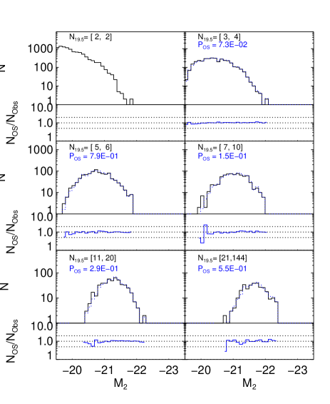
Figure 5.— The distributions of the $r$ band absolute magnitudes of the SGGs, i.e. the BSGs in six $N_{\rm 19.5}$ bins. The solid histogram shows the $M_{2}$ distribution of the real SGGs, while the dotted histogram shows that for the BSGs obtained from the OS prediction. The arrangement of the figure is the same as Fig. 4.

4. Modeling the magnitude distribution of BGGs

As shown above, the luminosity distribution of the BGGs are not consistent with the OS population expected from the CLF, while the SGGs are consistent with being the extremes of the satellite members expected from the CLF of satellite galaxies. These results suggest that BGGs are distinct from other member galaxies. In the current hierarchical structure formation model, BGGs are typically associated with the host haloes and located at the centers of their hosts, while other member galaxies are typically associated with dark matter subhaloes. Thus, being the centrals, BGGs may have the privilege to grow more during their evolution through galaxy cannibalism or through star formation fueled by cooling flows. Here, we test such a scenario using a toy model. We assume that the assembly history of a halo is only correlated with its halo mass, so that for groups with a given richness (halo mass), their members follow the same initial luminosity distribution function. After the BGGs settle into the group centers, they are assumed to be brightened by some environmental processes, while the luminosities of other members are assumed to remain unchanged. We denote the initial absolute magnitude of a BGG by $M^{*}_{1}$ and the subsequent change as $\Delta M$ ($>0$), so that the final magnitude of the BGG $M_{1}$ is written as

$$M_{1}=M^{*}_{1}-\Delta M.$$ (3)

The magnitudes of the other member galaxies remain unchanged, so that

$$M_{k}=M^{*}_{k}\,,$$ (4)

where $k$ is the rank order in luminosity of group members. In this scenario, the distributions of $M^{*}_{1}$ and $M_{k}(k=2,\cdot\cdot\cdot N_{\rm 19.5})$ are expected to follow the OS predictions of the same underlying (initial) distribution function, if the model for $\Delta M$ is correct. Thus, to test the model, we apply the reversed brightening process ($\Delta M$) to the observed BGGs ($M_{1}$) and check whether or not the ‘dimmed’ BGGs ($M^{*}_{1}$) is consistent with the OS prediction of the luminosity distribution of galaxies in the sample where BGGs are replaced by their ‘dimmed’ counterparts (referred to as the ‘BGG-dimmed’ sample). Moreover, to get further constraints on $\Delta M$, we may also check whether the magnitude of SGGs ($M_{2}$) and galaxies in other rank orders are consistent with the OS predictions based on the underlying distributions of the ‘BGG-dimmed’ sample.

In practice, for each $N_{\rm 19.5}$ bin we reduce the luminosity of each BGG by an amount of $\Delta M$, where $\Delta M$ is parameterized by some simple model parameters (to be specified later). In order to ensure that the BGG retains its brightest status after dimming, $\Delta M$ is constrained to be smaller than the observed magnitude gap, $G_{1,2}$, for any given group (to be discussed later). After this dimming, we make statistical tests on whether all the ordered members become being consistent with OS predictions. To do that, we apply a shuffling algorithm on the group members of this ‘BGG-dimmed sample’ within each $N_{\rm 19.5}$ bin. More specifically, we first assign all member galaxies of the ‘BGG-dimmed’ sample in a given richness bin into an array, $\{i=1,2,\cdot\cdot\cdot,N_{\rm gal}\}$, so that each group is represented by a set of integers equal to the indices assigned to their member galaxies. We then randomly shuffle the elements of the corresponding magnitude array $M_{i}$ so that each index is now associated with a new magnitude in the shuffled array. Finally we build a sample of new groups so that each group contains member galaxies specified by their original indices but with their magnitudes according to the shuffled magnitude array. Because the members of each new group are assigned in a statistical (random) way, the BGGs and the members at any other ranks can be considered as a statistical population of the primordial distribution (i.e. the distribution before the evolution of the BGGs).

For convenience, we refer these new groups as ‘shuffled groups’. Finally, we apply a non-parametric KS test to check the probabilities that the distributions of the‘BGG-dimmed’ sample, (e.g. $M^{*}_{1},M_{2}$) are consistent with those of the shuffled groups.

4.1. Average brightening of the brightest group galaxies

As a first step, we estimate the average brightening of the BGGs relative to that of other member galaxies. For a given $N_{\rm 19.5}$ bin, we assume that the BGG brightening is independent of any other group properties and can be parameterized by a simple parameter $\Delta M$. In principle, one can assume that the BGG brightening $\Delta M$ has some random scatter.However, we have found that our statistical model can not provide any constraints on this scatter. The reason is that any random scatters on the BGGs do not change the statistical nature of the BGGs and are degenerated with the random shuffling process. Therefore, the parameter $\Delta M$ we assumed in different $N_{\rm 19.5}$ bins is better to be understood as the average values of the BGG brightening rather than a constant. Nevertheless, we refer to this BGG brightening model parameterized by a constant $\Delta M$ as $C$ model below.

For a given $N_{\rm 19.5}$ bin and a given value of $\Delta M$, we calculate the KS test probabilities, $P_{\rm BGG}$ and $P_{\rm SGG}$, which are the $M^{*}_{1}$ and $M_{2}$ distributions of the BGG-dimmed sample follow the same distributions as those of the shuffled groups respectively. We define a combined KS test probability,

$$P_{\rm B,S}=P_{\rm BGG}*P_{\rm SGG}\,.$$ (5)

For each $N_{\rm 19.5}$ bin, we then search the best values of $\Delta M$ in the parameter space by maximizing $P_{\rm B,S}$. To reduce the statistical fluctuations during the shuffling process, we make the shuffling process 100 times for each assumed value of $\Delta M$, and use the mean of these 100 realizations to estimate the KS test probabilities.

In Fig. 6, we show the $P_{\rm BGG}$, $P_{\rm SGG}$ and $P_{\rm B,S}$ as function of $\Delta{M}$ for 6 different $N_{\rm 19.5}$ bins with the dotted, dashed and solid lines respectively. As one can see, we get very good estimates of $\Delta M$ (with $P_{B,S}>0.1$) in all richness bins. Although the constraint on $\Delta M$ mainly comes from the BGG distribution($P_{\rm BGG}$), the behavior of the SGG distribution($P_{\rm SGG}$) also shows good consistence.

For each $N_{\rm 19.5}$ bin, we define the best estimate of the average BGG brightening, $\Delta\bar{M}$, as the value at which the accumulated probability starting from $\Delta M=0$ is half of that from $\Delta M=0$ to $\Delta M=0.5$. This estimate matches the maximum $P_{\rm BS}$ estimation well in most of the cases, but is more robust. The uncertainties of the best estimates are then calculated from the 68 percentiles of the likelihood distribution on each side of $\Delta\bar{M}$. The values of $\Delta\bar{M}$ so obtained are $0.09$, $0.20$, $0.30$, $0.23$, $0.19$, $0.22$ magnitudes for six richness bins, respectively. They are plotted together with their uncertainties in the top panel of Fig. 7 and are listed in Table 1.

The actual average magnitudes we have used to dim the BGGs are slightly smaller than the values of $\Delta\bar{M}$, because we have forced $\Delta M<G_{1,2}$ so that each BGGs remains to be the brightest after the dimming. However, since the fraction of groups with $G_{1,2}<\Delta\bar{M}$ is quite small (see the bottom right panel of Fig. 1), the difference between the real average dimming and $\Delta\bar{M}$ is small, typically $\sim 0.01$ mag.

We may abandon the constraint $\Delta M<G_{1,2}$ in our model. However, we find that the value of $\Delta\bar{M}$ can no longer be strongly constrained by the observational data. The reason is, because then a galaxy at any rank can in principle become the BGG when $\Delta M$ is chosen sufficiently large. For example, consider a case in which the initial luminosities of the current BGGs are fainter than the third brightest group galaxies (TGGs) of the current groups. Thus, after the BGG-dimming, the SGGs of the current groups become the BGGs of the initial groups and the TGGs of the current groups become the SGGs of the initial groups. Since the distributions of the SGGs and TGGs of the current groups are consistent with the OS prediction(Section 3.2), such a scenario is also acceptable if we give up the assumption $\Delta M<G_{1,2}$.

Except the lowest $N_{\rm 19.5}=2$ bin, the average BGG brightening $\Delta\bar{M}$ is roughly a constant $\sim 0.2$ mag. Using the $N_{\rm 19.5}-M_{\rm h}$ relation in Equ. 2, we label the median $M_{\rm h}$ of the groups in 6 $N_{\rm 19.5}$ bins on the top axis of Fig. 7. We see that the $N_{\rm 19.5}>2$ groups corresponds to the haloes with $M_{\rm h}>10^{13}h^{-1}M_{\odot}$.

It is worthy to mention that the low $N_{\rm 19.5}$ groups are not complete in halo mass(see Fig. 2). There are low mass groups with all their members/satellites $M_{\rm r}$ fainter than $-19.5$ mag. Such groups have $N_{\rm 19.5}=0/1$ by definition. The BGGs of these $N_{\rm 19.5}<2$ groups may also over-grow their stellar masses through, e.g. cannibalizing the very faint satellites($M_{\rm r}<-19.5$ mag). However, our OS studies requires at least two members for each group and can not be applied to them .

To get the implication on how large is the BGG brightening for these $N_{\rm 19.5}<2$ groups, one way is to go to a sample of groups with deeper magnitude limit. With a lower magnitude limit to the member galaxies, some of the $N_{\rm 19.5}<2$ groups become to have more than two members and so that the OS studies can be applied. We provide such an analysis in Appendix A, where we select a sample of lower redshift groups with members complete to $M_{\rm r}<-18.5$ mag. By including fainter members, we show that the BGGs of $N_{\rm 19.5}<2$ groups also have experienced a significant brightening process, i.e. $\Delta M>0$. Moreover, we further show that the brightening process of the BGGs of the low mass groups varies among different groups and shows complicate dependence on the group richness parameters. The physics behind this variety is that, the BGG growth history depends on its real halo mass and environment, while for the low mass halos, any single observable parameter is not adequate to characterize its real halo mass and/or environment. We will leave a detailed discussion of the dependence of $\Delta M$ on the group properties in a forthcoming paper.

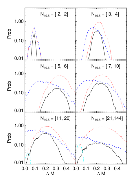
Figure 6.— The KS test probabilities $P_{\rm BGG}$, $P_{\rm SGG}$ and $P_{\rm B,S}$ as function of the average BGG brightening $\Delta M$ for 6 different $N_{\rm 19.5}$ bins, which are shown by the dotted, dashed and solid lines in each panel respectively. The dot-dashed lines in bottom two panels show the KS test probability $P_{\rm GAP}$(see Section 4.3). For the other $N_{\rm 19.5}$ bins, $P_{\rm GAP}<0.01$ at all $\Delta M$ values and therefore are not shown.

4.2. The average stellar mass increment of the brightest group galaxies

The systematic brightening of BGGs may be caused either by extra star formation (which makes them bluer and brighter) or by an increase in stellar mass. In order to partly distinguish these two possibilities we also carry out modeling in terms of the stellar masses of the BGGs. In the group catalog used here, the stellar mass ($M_{\rm s}$) of each group member galaxy was obtained from the relation between the stellar mass-to-light ratio and the color (Bell et al., 2003). We thus make a similar study on the mass distribution of the most massive galaxies (MMGs) as we have done for the BGGs by assuming that all MMGs have increased their stellar masses on average by amounts $\Delta{\rm log}M_{\rm s}$ in logarithm unit. Since the analysis is parallel with that for BGGs, the details are given in Appendix B.

Here we make use of the groups whose MMGs are also the BGGs (99% of the cases), and plot the best estimate of the average mass increment $\Delta{\rm log}\bar{M}_{\rm s}$ as a function of group halo mass $M_{\rm h}$ in the top panel of Fig. 7. The error-bars also represent the 68 percentiles of the likelihood distribution at each side of the best estimate. Note that the ranges of the left vertical axis ($\Delta\bar{M}$ ) and the right vertical axis ($\Delta{\rm log}\bar{M}_{\rm s}$) of the top panel of Fig. 7 are $0.0-0.625$ mag and $0.0-0.25$ dex, respectively, and so the results show that the values of $\Delta\bar{M}$ and $\Delta{\rm log}\bar{M}_{\rm s}$ are consistent, suggesting that the brightening of BGGs is mainly caused by the increase in stellar mass. The amount of average mass increment is about twenty percent, $\Delta{\rm log}\bar{M}_{s}\sim 0.09$, for the massive haloes with $M_{\rm h}>10^{13}h^{-1}M_{\odot}$. For the low mass haloes in the lowest richness bin, the stellar mass increment is also lower, about 10 percent ($\Delta{\rm log}\bar{M}_{s}\sim 0.05$). Again, we caution that our low mass groups are not complete when in terms of halo mass.

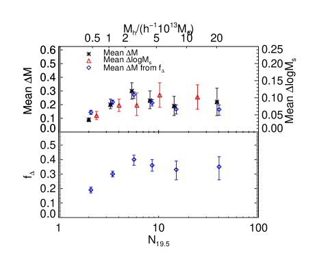
Figure 7.— The best estimates of the average magnitude brightening $\Delta\bar{M}$ of the BGGs as functions of the $N_{\rm 19.5}$ and host halo mass (top panel). Stars represent $\Delta\bar{M}$ estimated from the constant BGG brightening model (Section 4.1), while the diamonds show that estimated from the gap dependent BGG brightening model (Section 4.4). The triangles show the average stellar mass increment $\Delta{\rm log}\bar{M}_{s}$ of the MMGs (labelled on the right vertical axis) (Section 4.2). Bottom: The best estimate of $f_{\Delta}$ in the gap-dependent BGG brightening model (Section 4.4).

4.3. The magnitude gap $G_{1,2}$ distribution

So far we have studied on average how much BGGs are brightened by modeling the absolute magnitude distributions of the BGGs and SGGs together. In this subsection we study how the brightening is correlated with the other group properties. e.g. the magnitude gap $G_{1,2}$. The distribution of $G_{1,2}$ and its correlation with the host halo mass have been explored by many recent studies(More, 2012; Paranjape & Sheth, 2012; Tal et al., 2012). Some studies find that the $G_{1,2}$ distribution may contain dynamical information of the groups that is not contained in the group richness and BGG luminosity (Hearin et al., 2013a, b).

If we have a model that describes how BGG is brightened in individual groups, we will be able to explain not only the $M_{1}$ and $M_{2}$ distributions but also the distribution of the magnitude gap $G_{1,2}$. However, we find that the $G^{*}_{1,2}\equiv(M_{2}-M^{*}_{1})$ distribution can not be reproduced by our best constant BGG brightening model. For the best estimates of $\Delta\bar{M}$ in Section 4.1, the KS test probability $P_{\rm GAP}$(the $G^{*}_{1,2}$ distribution follows the same distribution as the shuffled groups) is nearly zero ($<10^{-5}$) for all richness bins. Moreover, except the two highest $N_{\rm 19.5}$ bins that have relative low statistical significance, we can not find any values of $\Delta M$ in the constant BGG brightening model which could make $P_{\rm GAP}>0.01$ (see the dot-dashed lines in Fig. 6). This result implies that our simple constant BGG brightening model is too simplistic to account for individual brightening. The inability of the constant brightening model in reproducing the $G^{*}_{1,2}$ distribution can be understood in another way. If we assume that the initial $G^{*}_{1,2}$ distribution follows the OS, it will always peak at $G^{*}_{1,2}=0$ for any Schechter-like CLFs of group members (e.g. Paranjape & Sheth, 2012). If all initial BGGs are then brightened by an amount of $\Delta\bar{M}$ in the subsequent evolution, the final $G_{1,2}$ distribution will peak at $\Delta\bar{M}$, in contrast to the observed $G_{1,2}$ distribution, which still peaks around 0(see bottom right panel of Fig. 1).

4.4. Magnitude gap-dependent brightening of the brightest groups galaxies

As a simple gap-dependent model, we assume that the brightening magnitude $\Delta M$ of each BGG is proportional to the magnitude gap $G_{1,2}$ of its host group,

$$\Delta M=f_{\Delta}*G_{1,2}$$ (6)

where the coefficient $f_{\Delta}$ is a model parameter to be determined. To distinguish this model from the constant brightening model in Section 4.1, we refer it as the $G$ model in the following.

In general, if a group has a larger initial gap $G^{*}_{1,2}$, its BGG is more dominant within the group. The more dominant BGG potentially has the ability to grow more through e.g. galaxy cannibalism. Thus, the observed $G_{1,2}$ becomes even larger. With the parametrization of Equ. 6, the value of $f_{\Delta}$ lies in between 0 and 1. The limit $f_{\Delta}=0$ is the case that there is no BGG brightening at all. On the other hand, the limit $f_{\Delta}=1$ means that the observed magnitude gap $G_{1,2}$ is totally contributed by the BGG brightening process.

As in Section 4.1, we apply a gap dependent dimming model to the BGGs in each $N_{\rm 19.5}$ bin. For any given values of $f_{\Delta}$, the BGGs are dimmed by $\Delta M$ using Equ. 6. We then make OS predictions for the $M^{*}_{1}$, $M_{2}$ and $G^{*}_{1,2}$ distributions by shuffling group members as that done in Section 4.1. We explore the parameter space of $f_{\Delta}$ by calculating the combined KS probability,

$$P_{\rm B,S,G}=P_{\rm BGG}*P_{\rm SGG}*P_{\rm GAP}\,,$$ (7)

where $P_{\rm BGG}$, $P_{\rm SGG}$ and $P_{\rm GAP}$ are the KS probabilities that the distributions of the BGG magnitudes, SGG magnitudes and magnitude gaps of the BGG-dimmed sample follow the OS predictions respectively. Compared with $P_{\rm B,S}$(Equ. 5) used for the $C$ model in Section 4.1, the new model uses the $G^{*}_{1,2}$ distribution as an extra constraint.

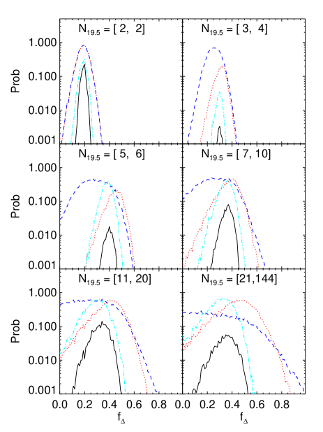
Figure 8.— The KS test probabilities as function of $f_{\Delta}$ for 6 different $N_{\rm 19.5}$ bins. The dotted, dashed and dot-dashed lines show the probabilities$P_{\rm BGG},P_{\rm SGG},P_{\rm GAP}$ respectively, while the solid lines show the combined probability $P_{\rm B,S,G}$ (see Section 4.4 for detail)

We show the $P_{\rm B,S,G}$ as function of $f_{\Delta}$ with solid lines for different $N_{\rm 19.5}$ bins in Fig. 8, whereas the $P_{\rm BGG}$, $P_{\rm SGG}$ and $P_{\rm GAP}$ are shown by the dotted, dashed and dot-dashed lines respectively. Remarkably, the constraints from the BGGs($P_{\rm BGG}$), SGGs($P_{\rm SGG})$ and the magnitude gap($P_{\rm GAP}$) on this gap dependent BGG brightening model are in good consistence with each other. As in Section 4.1 , we take the value of $f_{\Delta}$, where the accumulated $P_{\rm B,S,G}$ from $f_{\Delta}=0$ is half of the accumulated $P_{\rm B,S,G}$ from $f_{\Delta}=0$ to $f_{\Delta}=1$, as the best model estimate. The 68 percentiles on each side of the best model are then used as the error estimates. The best estimates of $f_{\Delta}$ are about $0.2$-$0.4$, with weak dependence on $N_{\rm 19.5}$. They are plotted in the bottom panel of Fig. 7 and listed in Table 1.

For each richness bin, we also calculate the average BGG dimming/brightening from Equ. 6 using the best estimates of $f_{\Delta}$ and plot them as the open diamonds in the top panel of Fig. 7, where the error-bars are obtained from the error estimates of $f_{\Delta}$. As we can see, the average BGG dimming/brightening of the $G$ model is in excellent agreement with that of the $C$ model in Section 4.1. Moreover, because of the further constraint from the $G^{*}_{1,2}$ distribution, the constraints on the average BGG brightening in the $G$ model are tighter than that in the $C$ model .

To have a better visualization of our gap dependent BGG brightening model, we make predictions for the $M_{1}$, $M_{2}$ and $G_{1,2}$ distributions as functions of $N_{\rm 19.5}$, and compare them with the corresponding observational results. To do this, we first construct a ‘BGG-dimmed’ sample using the best model of $f_{\Delta}$ for each $N_{\rm 19.5}$ bin. We then use the $M_{\rm r}$ distributions of the ‘BGG-dimmed’ sample as the primordial CLFs of the group members. These primordial CLFs are shown as the solid histograms in Fig. 9, where the observed CLFs (already shown as the solid histograms in Fig. 3) are shown as the dotted histograms for comparison. For reference, we also plot the luminosity distribution of the single galaxies as the dashed curve in each panel after normalized to the same number of the group members in the corresponding $N_{\rm 19.5}$ bin. By comparing with the luminosity distribution of the single galaxies, we see that, after considering the BGG brightening in different $N_{\rm 19.5}$ bins, the primordial CLF still changes systematically with group richness , in the sense that group members are also on average brighter in groups with higher richness.

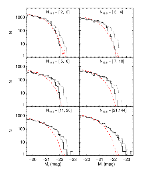
Figure 9.— The primordial conditional luminosity function of the group members in six $N_{\rm 19.5}$ bins (solid histograms). In each panel, the dotted histogram show the observed conditional luminosity function, while the dashed line show the luminosity function of the single galaxies which has been normalized to the number of the group members in that richness bin.

With the primordial CLFs in different $N_{\rm 19.5}$ bins, we generate 100,000 mock groups for each $N_{\rm 19.5}$ using a Monte-Carlo method, and obtain $M^{*}_{1}$ and $M_{2}$ for each mock group by sorting the group members in luminosity ranks. Next, we brighten $M^{*}_{1}$ of each mock group with an amount of

$$\Delta M=f_{\Delta}/(1-f_{\Delta})*G^{*}_{1,2}\,,$$ (8)

where $f_{\Delta}$ takes the best estimate shown in Fig. 7. In Equ. 8, $G^{*}_{1,2}$ is the magnitude gap of the OS sample, i.e. the gap before the BGG brightening, so that Equ. 8 takes a different formulism from Equ. 6. These new mock groups after BGG brightening are referred to as the model groups, and have $M_{1}=M^{*}_{1}-\Delta M$ and $G_{1,2}=G^{*}_{1,2}+\Delta M$. We then calculate the mean and dispersion of the $M_{1}$, $M_{2}$ and $G_{1,2}$ distributions of the model groups for each $N_{\rm 19.5}$. The mean and dispersion so obtained as functions of $N_{\rm 19.5}$ and $M_{\rm h}$ are plotted as the solid lines in Fig. 10, 11,12, respectively. Eq. (2) is used in converting $N_{\rm 19.5}$ to $M_{\rm h}$. Since the number of model groups for each $N_{\rm 19.5}$ is large, their statistical fluctuation is small. For comparison, the results of the real groups are plotted as the triangles in these figures. In Fig. 10 and 12, we also plot the results of the model groups before the BGG brightening (i.e. OS model predictions) as the dashed lines. As one can see, after applying a simple BGG brightening, the distributions of $M_{1}$ and $G_{1,2}$ both become in good agreement with the observed distributions. For the SGGs shown in Fig. 11, there are excellent agreements between the observations and OS predictions. Similar conclusions have already been shown in Fig. 5. However, these two plots have different implications. Fig. 5 shows that the SGGs are consistent with the extreme value distribution of the satellite population and are independent of the BGGs. Here in Fig.11, on the other hand, the SGGs and BGGs are assumed to originate from the same population, and the SGGs are in good consistence with OS predictions after the BGG brightening has been taken into account.

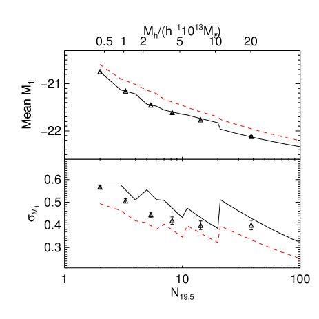
Figure 10.— The mean and scatter of the magnitude of BGGs ($M_{1}$) as function of $N_{\rm 19.5}$ and $M_{\rm h}$. The abscissa of $M_{\rm h}$ is labelled on top of the figure. The triangles show the results of our real groups. The dashed lines show the model prediction from OS, while the solid lines show the results after applying a gap-dependent BGG brightening.

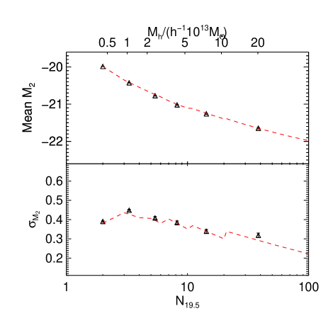
Figure 11.— The mean and scatter of the magnitude of SGGs $M_{2}$ as function of $N_{\rm 19.5}$ and $M_{\rm h}$. The triangles show the results of our real groups, while the dashed lines show our model prediction from OS.

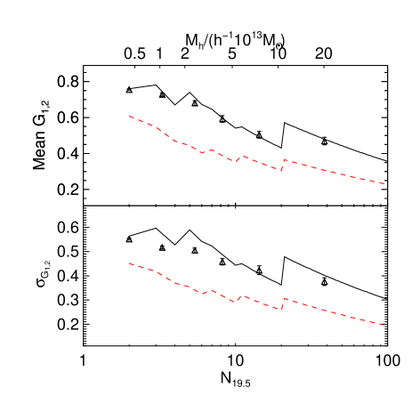
Figure 12.— The mean and scatter of the magnitude gap $G_{1,2}$ as function of $N_{\rm 19.5}$ and $M_{\rm h}$. The triangles show the results of our real groups. The dashed lines show the model prediction from OS, while the solid line shows the results after applying a gap-dependent BGG brightening.

5. The Tremaine-Richstone test

Tremaine & Richstone (1977) defined two parameters to test the statistical nature of BGGs (hereafter TR tests) using the dispersion of the absolute magnitude of the BGGs, $\sigma_{\rm M_{1}}$, and the mean ($\bar{G}_{1,2}$) and dispersion ($\sigma_{\rm G_{1,2}}$) of the magnitude gap $G_{1,2}$:

$$T_{1}\equiv\frac{\sigma_{\rm M_{1}}}{\bar{G}_{1,2}}\,;$$

$$T_{2}\equiv\frac{\sigma_{\rm G_{1,2}}}{\bar{G}_{1,2}}\,.$$ (9)

For the tail-end of a statistical distribution with an exponential decay, Tremaine & Richstone (1977) showed that these two test parameters have $T_{1}\geq 1$ and $T_{2}\geq 0.82$. That means, if the BGGs are drawn from the same population as the other members, the expected magnitude gap $\bar{G}_{1,2}$ should be smaller than the scatter of the BGG magnitudes and be of the same order as its own dispersion. The TR tests are not sensitive to the shape of the assumed luminosity function (except the exponential decay) and the variation from cluster to cluster, so are widely used to test whether the brightest cluster galaxies are consistent with an extreme value population (Geller & Postman, 1983; Postman & Lauer, 1995; Loh & Strauss, 2006; Lin et al., 2010). However, the applicability of the TR tests has not been validated for the low mass/richness groups.

Figure 13.— The TR-test parameters as function of group richness. The left, middle and right panels show the results for different group samples. In each panel, the triangles show the TR parameters of the group sample in different richness bins, while the solid line shows the statistical model prediction from Monte-Carlo simulations. The horizontal lines show the critical values of Tremaine & Richstone (1977). Left: real groups; Middle: groups whose BGGs have been dimmed by the best $C$ model (Section 4.1); Right: groups whose BGGs have been dimmed by the best $G$ model (Section 4.4).

We carry out the TR tests for three different group samples. The first is the real group sample. The second is the group sample with the BGGs dimmed using the best $C$ model (Section 4.1), while the third one is the group sample whose BGGs are dimmed using the best $G$ model (Section 4.4). All three group samples are also divided into six $N_{\rm 19.5}$ bins as before. The TR test values are calculated for groups within each $N_{\rm 19.5}$ bin, and the results are shown as the triangles in Fig. 13, with the left, middle and right panels showing the results for the three different samples, respectively. The error-bars of the TR-tests are estimated from 100 boot-strap re-samplings.

For each sample, we also calculate the values of TR parameters predicted by the OS as functions of group richness with Monte-Carlo simulations. Specifically, we generate 100,000 random groups for each $N_{\rm 19.5}$, as is done in Section 4.4. Note that the underlying distributions of these three group samples are different and our OS predictions are made in a self-consistent way. The values of the TR parameters predicted by the OS as functions of $N_{\rm 19.5}$ are shown as the solid line in each panel of Fig. 13. Again, because of the large size of the Monte-Carlo sample, the uncertainties of the predicted values are negligible. The critical TR test values suggested for rich clusters by Tremaine & Richstone (1977) , $T_{1}=1$, and $T_{2}=0.82$ are shown as the dotted horizontal lines in each panel.

As one can see from the solid lines in different panels of Fig. 13, the dependence of the OS predictions on the underlying distributions is quite weak. This result confirms that the TR test is not sensitive to the shape of the luminosity function of the group members. However, there is a weak dependence of the test parameters on the group richness. Both $T_{1}$ and $T_{2}$ increase monotonically but slowly with richness and approach their asymptotic values at $N_{\rm 19.5}>30$. The two criteria, $T_{1}\geq 1$ and $T_{2}\geq 0.82$, are achieved only at $N_{\rm 19.5}>10$, while the expectation values $T_{1}=1.29$ and $T_{2}=1$ suggested by Bhavsar & Barrow (1985) are not achieved even at $N_{\rm 19.5}=100$.

For the real groups, $T_{1}$ is systematically smaller than the statistical model prediction, while $T_{2}$ shows agreement with the model (left panels of Fig. 13). Because BGGs are expected to have experienced brightening, the mean magnitude gap $\bar{G}_{1,2}$ of the real groups are systematically larger than the OS prediction (Fig. 12 ). As a result, $T_{1}$ is systematically smaller than the OS prediction. On the other hand, since the scatter in the $G_{1,2}$ of the real groups is also systematically larger than the OS prediction (Fig. 12), the test parameter $T_{2}$ appears consistent with the OS prediction. Because of this coincidence, different answers can be obtained by using different TR tests for high-richness groups. This has been noticed by Lin et al. (2010), who found that the BGGs of high-mass clusters are not consistent with a statistical sample based on $T_{1}$, but are consistent when $T_{2}$ is used.

For the two different BGG-dimmed samples, the TR test values are quite different. For the constant BGG dimming model (middle panels, $C$ model in Section 4.1), $T_{1}$ is consistent with the OS prediction, while $T_{2}$ becomes systematically larger than the OS prediction. For the gap-dependent BGG dimming model (right panels, $G$ model in Section 4.4), both of the test parameters are roughly consistent with the OS predictions. The different behaviors of the two BGG-dimmed models are mainly caused by the way how the BGGs are dimmed. For the $C$ model, the BGGs are dimmed by a richness-dependent constant, the scatter in $G_{1,2}$ is thus roughly preserved, so that the value of $T_{2}$ increases systematically due to the BBG dimming. For the $G$ model, on the other hand, the mean and scatter of $G_{1,2}$ are both decreased due to the gap-dependent dimming, so that the values of $T_{2}$ remain unchanged after BGG dimming. This can be understood in another way, the $T_{2}$ values of primordial groups before the BGG brightening are expected to be consistent with the OS prediction. Thus, only when the BGG brightening process changes the mean and scatter of $G_{1,2}$ in a similar manner, can the $T_{2}$ values of the evolved groups remain consistent with the OS prediction. In this sense, the agreement shown in the lower left panel of Fig. 13 may not be a coincidence, but is a result of how BGGs are brightened.

Given these different behaviors of $T_{1}$ and $T_{2}$, it seems that $T_{1}$ is more useful than $T_{2}$ in testing whether BGGs are consistent with the OS, while $T_{2}$ may be useful in testing the details how the BGGs are brightened.

6. Summary

In this study, we test the statistical hypothesis of BGGs using a large sample of groups of galaxies selected from the DR7 of SDSS. We define a richness parameter $N_{\rm 19.5}$, the number of the group members with $M_{\rm r}<-19.5$ mag, to parameterize the host halo mass of each group. By dividing the groups into different $N_{\rm 19.5}$ bins, we measure the conditional luminosity distribution of the group members and build the corresponding statistical sample of groups by Monte-Carlo simulations. By comparing the real groups and the statistical sample, we study the statistical properties of the BGGs and other members. Our results can be summarized as follows:

• The BGGs are systemically brighter than the OS model prediction, which can be explained by a special BGG brightening process.

• To make the distribution of the BGG luminosities consistent with the EVS, the BGGs on average have to be dimmed by about $\sim 0.2$ mag.

• Taking into account the BGG brightening, the luminosity distribution of the SGGs is in good agreement with the OS.

• To simultaneously reproduce the distributions of the magnitudes of BGG, SGG and their gap, the brightening of a BGG should be correlated with the gap $G_{1,2}$ (or $G^{*}_{1,2}$). Such a brightening will boost $G^{*}_{1,2}$ by an amount of $\sim 50$ percent relative to the EVS of the underlying distribution.

The above results may provide some insight into the formation and evolution of the BGGs. The BGGs may have originated from the same statistical processes as other bright galaxies. On top of that, BGGs should also have experienced some brightening process which not be experienced by other bright galaxies. The brightening is mainly due to the growth of stellar mass, and may be related to local processes, such as galactic cannibalism and/or star formation in cooling flows. On average, the excess over the expectation of the EVS is about 20 percent for groups with halo masses $M_{\rm h}>10^{13}h^{-1}M_{\odot}$. The excess of stellar mass of a BGG is more significant if itself is more prominent inside its group. Such a scenario is in good agreement with the evolution of BGGs through minor mergers (e.g. Edwards & Patton, 2012).

In such a scenario, the BGGs are the central galaxies in groups. However, as shown by Skibba et al. (2011), the BGGs may not always be the centrals. The fraction of non-central BGGs may be as high as 25 to 40 percent. We have tested such a possibility by assuming that a fraction of BGGs, $f_{\rm BNC}$, are not the centrals and so have not experienced any brightening effects (i.e. $\Delta M$=0). We find such a scenario is also acceptable, but our statistical model cannot provide any strong constraint on $f_{\rm BNC}$ could be. In the test we have also assumed that the current BGGs are the initial BGGs. It is also possible that an initial central galaxy is not the BGG but becomes the BGG only after the brightening process. For the $C$ model, our statistical data cannot provide any constraints on such a possibility, as discussed in Section 4.1. Such a scenario is not compatible with the $G$ model by definition. Finally, we emphasize again that our results are statistical. How much the BGGs are brightened for specific groups may depend on the details of their formation processes(as we haven shown in Appendix A). In a future paper, we will divide groups into subsamples according to intrinsic properties in addition to group richness, and examine how the growth of the BGGs may depend on these other properties.

Table 1The average halo mass $M_{\rm h}$, the number of groups $N_{\rm{gro}}$, the number of group members $N_{\rm{gal}}$, the best estimations of model parameters $\Delta\bar{M}$(Section 4.1), $f_{\Delta}$(Section 4.4) in six $N_{\rm 19.5}$ bins.

$N_{\rm 19.5}$	2-2	3-4	5-6	7-10	11-20	21-144
$N_{\rm{gro}}$	9,817	3,620	1,013	765	494	305
${\rm log}\,M_{\rm h}$	12.61	13.05	13.41	13.63	13.88	14.30
$N_{\rm{gal}}$	19,634	11,958	5,457	6,261	7,072	11,699
$\Delta\bar{M}$	$0.09^{+0.01}_{-0.01}$	$0.20^{+0.03}_{-0.04}$	$0.30^{+0.06}_{-0.06}$	$0.23^{+0.07}_{-0.06}$	$0.19^{+0.07}_{-0.07}$	$0.22^{+0.10}_{-0.10}$
$f_{\Delta}$	$0.19^{+0.02}_{-0.02}$	$0.30^{+0.02}_{-0.02}$	$0.40^{+0.03}_{-0.04}$	$0.36^{+0.04}_{-0.04}$	$0.33^{+0.06}_{-0.07}$	$0.35^{+0.09}_{-0.09}$

Appendix A The group richness $N_{18.5}$

In this section, we test the BGG brightening model with a new sample of groups whose complete magnitude limit reaches to $-18.5$ mag by applying a lower redshift limit ($z<0.506$) to the group catalog of Yang et al. (2007). Similar as $N_{\rm 19.5}$, $N_{18.5}$ is defined as the number of the group members brighter than $-18.5$ mag. In the DR7 version of the group catalog of Yang et al. (2007), there are 54,497 groups with $N_{18.5}\geq 1$ at $z<0.506$. The number of their members is 80,761. We name this new group sample as the $N_{18.5}$ groups so as to be distinguished from the $N_{\rm 19.5}$ groups we used in the main text. Because of the including of the fainter members, the richest group now has $N_{18.5}=284$.

For the $N_{18.5}$ groups, we calculate both $N_{18.5}$ and $N_{\rm 19.5}$ for each group. In Fig. 14, we plot their $N_{\rm 19.5}$ versus $N_{18.5}$ . At each $N_{\rm 19.5}$ , we calculate the mean $N_{18.5}$ and plot them as the triangles. As we can see, there is a tight correlation between$N_{18.5}$ and $N_{\rm 19.5}$ for high richness groups. For the low richness groups, there are significant scatters between each other. For the $N_{\rm 19.5}$ groups in the main text, all of them have $N_{\rm 19.5}\geq 1$ . However, for the $N_{18.5}$ groups, there are a significant fraction of groups with $N_{\rm 19.5}=0$ . These are the groups with all their members fainter than $-19.5$ mag but with at least one member brighter than $-18.5$ mag. The number of such $N_{\rm 19.5}=0$ groups is as high as 26,625 and their $N_{18.5}$ ranges from 1 to 4. Also, because the $N_{\rm 19.5}=0$ groups have no member brighter than $-19.5$ mag, no halo mass has been estimated in the group catalog of Yang et al. (2007).

We fit a power law relation between $N_{18.5}$ and $N_{\rm 19.5}$ for $N_{\rm 19.5}>0$ groups and obtain

$$N_{18.5}=1.44N_{19.5}^{1.08}\,.$$ (A1)

This fitting relation is shown as the solid line in Fig. 14. As we can see, this relation fits the mean $N_{18.5}$ as function of $N_{\rm 19.5}$ very well.

Figure 14.— The correlation between $N_{18.5}$ and $N_{\rm 19.5}$ for the $N_{18.5}$ groups . The triangles show the mean $N_{18.5}$ at each given $N_{\rm 19.5}$. The solid line shows the fitting line of Equ. A1

.

To test our BGG brightening model with the new $N_{18.5}$ sample, we make analysis on the average BGG brightening($\Delta\bar{M}$) using the same algorithm as that in Section 4.1.We bin the $N_{18.5}$ groups into 4 $N_{18.5}$ bins( [2,2], [3,5], [6,10], [11,274]), where the numbers of the groups are 5069, 2148, 519 and 441 respectively. The best estimates $\Delta\bar{M}$ for the groups in the four bins are 0.18, 0.34, 0.33 and 0.32 mag respectively. To compare with the results of $N_{\rm 19.5}$ groups in Section 4.1, we show the $\Delta\bar{M}$ as function of their average $N_{\rm 19.5}$ for the $N_{18.5}$ groups as the triangles in Fig. 15. The results of $N_{\rm 19.5}$ groups in Section 4.1 so that are plotted as the open squares for comparison.

As we can see, for the high richness groups, the $\Delta\bar{M}$ from the $N_{18.5}$ groups are in consistence with the $N_{\rm 19.5}$ groups. However, for the low richness groups, the results show discrepancy. The $\Delta\bar{M}$ of the $N_{\rm 19.5}=2$ groups is $\sim 0.1$ mag, whereas the $\Delta\bar{M}$ of the groups in the $N_{18.5}=[3,5]$ bin is $\sim 0.3$ mag although their average $N_{\rm 19.5}$ is also about 2. This discrepancy is caused by the fact that there are significant scatters between $N_{18.5}$ and $N_{\rm 19.5}$ for the low richness groups. For example, although the mean $N_{\rm 19.5}$ of the groups in the $N_{18.5}=[3,5]$ bin is close to 2, their $N_{\rm 19.5}$ ranges are from 0 to 5. There are 2148 groups within the $N_{18.5}=[3,5]$ bin, however, only less than half of of them(893) have $N_{\rm 19.5}=2$.

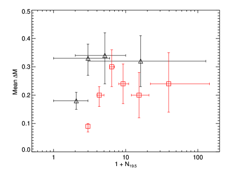
Figure 15.— The average BGG brightening($\Delta\bar{M}$) of the groups as function of $N_{\rm 19.5}$. The triangles show $\Delta\bar{M}$ of the groups in 4 $N_{18.5}$ bins, while the squares show the groups in 6 $N_{\rm 19.5}$ bins (see Fig. 7). The vertical error-bars show the 68 percentiles of the likelihood distribution, while the horizontal error-bars represent the $N_{\rm 19.5}$ ranges of the groups in each given bin.

Besides the large scatter between $N_{\rm 19.5}$ and $N_{18.5}$, the large discrepancy in $\Delta\bar{M}$ for the low richness group may also imply that the growth of the BGGs may not depend on any single richness parameter ($N_{18.5}$ or $N_{\rm 19.5}$) in a simple way. To show this, we make an analysis on the dependence of $\Delta M$ on both $N_{18.5}$ and $N_{\rm 19.5}$. In the $N_{18.5}$ group sample, there are 2,225 groups with $N_{\rm 19.5}=2$ and their $N_{18.5}$ range from 2 to 11. For these $N_{\rm 19.5}=2$ groups, a group with $N_{18.5}=2$ means that their is no group member with luminosity between $-19.5$ and $-18.5$ mag. On the other hand, a group with $N_{18.5}=11$ means it has 9 members within the luminosity range $-19.5<M_{r}\leq-18.5$. Therefore, our test is whether the brightening of the BGGs is correlated with the number of the group members in between $-19.5<M_{r}\leq-18.5$.

We divide the above 2,225 $N_{\rm 19.5}=2$ groups into four sub-samples according to their $N_{18.5}$ values. The four sub-samples are the groups with $N_{18.5}$ being 2,3,4 and $>4$ respectively. The number of the groups in these four sub-sample are 1270, 573, 232 and 150 accordingly. We estimate the $\Delta\bar{M}$ of the BGGs for these 4 $N_{\rm 19.5}=2$ sub-samples using the same algorithm as that in Section 4.1. The best estimates of the $\Delta\bar{M}$ of these 4 sub-samples are shown in Fig. 16. As can be seen, although all the sub-samples have $N_{\rm 19.5}=2$, the $\Delta\bar{M}$ shows a strong dependence on $N_{18.5}$. The $\Delta\bar{M}$ is systematically larger for the groups with larger $N_{18.5}$. The sub-sample of the groups with $N_{18.5}=2$ is the majority of the global $N_{\rm 19.5}=2$ sample(1270 of 2225), which might be the reason that the $\Delta M$ of this sub-sample is close to the result of the general $N_{\rm 19.5}=2$ sample(Section 4.1, $\sim 0.1$ mag). The increase of $\Delta\bar{M}$ with the increasing number of faint members($-19.5<M_{r}\leq-18.5$) might be qualitatively explained by that the BGGs can grow more through cannibalization if they have more faint satellites. However, a quantitative explanation needs a more detailed modeling of the growth of the BGGs. We will leave such a detailed study in forthcoming.

Figure 16.— The average BGG brightening($\Delta\bar{M}$) of the $N_{\rm 19.5}=2$ groups as function of their $N_{18.5}$.

Appendix B The most massive galaxies of groups

As described in Yang et al. (2007), the stellar mass of all group member galaxies have been computed using fitting formula of Bell et al. (2003),

$${\rm log}[M_{\rm s}/(h^{-2}M_{\odot})]=-0.406+1.097[^{0.0}(g-r)]-0.4(^{0.0}M_{\rm r}-5{\rm log}h-4.64)\,,$$ (B1)

where ${}^{0.0}(g-r)$ and ${}^{0.0}M_{\rm r}$ are the SDSS $g-r$ color and $r$ band absolute magnitude $K$-corrected and evolution corrected to redshift $z=0.0$.

As given redshift $z$, for the SDSS main galaxy sample, the galaxies are volume complete at the stellar mass limit ${\rm log}[M_{\rm{\rm s,lim}}]$. van den Bosch et al. (2008) obtained a fitting relation of the stellar mass limit $M_{\rm s,lim}$ as function of redshift $z$,

$${\rm log}[M_{\rm{\rm s,lim}}/(h^{-2}M_{\odot})]=\frac{4.852+2.246{\rm log}D_{L}(z)+1.123{\rm log}(1+z)-1.186z}{1-0.067z}$$ (B2)

where $D_{L}(z)$ is the luminosity distance at redshift $z$. For us, we select the groups with redshift $z<0.075$ and so that obtain a volume complete sample of members down to stellar mass $M_{\rm s}\sim 3\times 10^{10}h^{-2}M_{\odot}$. The stellar-mass-defined group richness $N_{s}$ is accordingly defined as the number of members with stellar mass higher than $3\times 10^{10}h^{-2}M_{\odot}$. We show the correlation between $N_{s}$ and host halo mass $M_{\rm h}$ in Fig. 17.

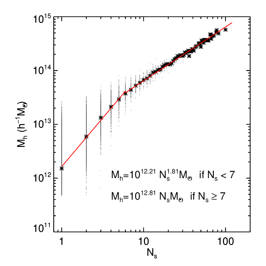
Figure 17.— The correlation between the stellar-mass-defined group richness$N_{\rm s}$ and host halo mass. The dashed line shows the fitting relation of equation B3.

We also fit a broken power-law relation between $M_{\rm h}$ and $N_{\rm s}$ with the break point at $N_{\rm s}=7$. For high richness groups($N_{\rm s}\geq 7$), we fix the power law index $n=1$. While for low richness groups($N_{\rm s}<7$), we get the power law index $n=1.81$ from a least square fitting of the linear relation between ${\rm log}M_{\rm h}$ and ${\rm log}N_{\rm s}$. The resulted fitting formula is shown as equation (B3) and plotted as the solid line in Fig. 17.

$$M_{\rm h}=\left\{\begin{array}[]{ll}10^{12.21}\,N_{\rm s}^{1.81}\,h^{-1}M_{\odot}&\mbox{if $N_{\rm s}<7$}\\ 10^{12.81}\,N_{\rm s}\,h^{-1}M_{\odot}&\mbox{if $N_{\rm s}\geq 7$}\end{array}\right.$$ (B3)

As for BGGs, we test the model that the most massive galaxies(MMGs) of groups are initially a statistical population, and then evolved with their stellar massed increased. We divide the group sample into 5 $N_{s}$ bins. The ranges of the 5 $N_{\rm s}$ bins are [2,2], [3,4], [5,6], [7,10], [11,100] respectively. We also parameterize the average stellar mass increment of MMGs in each richness bin with a simple parameter $\Delta{\rm log}M_{s}$. As that in Section 4.1, we also require $\Delta M_{s}$ can not be larger than the stellar mass difference between the MMG and the second most massive galaxy. We use KS test to check whether the distribution of the stellar masses of the MMGs and the second most massive galaxies are consistent with the ‘shuffled’ groups as that done in Fig. 6. We show the KS test probabilities $P_{\rm MMG}$, $P_{\rm SMG}$ and the combined probability ($P_{\rm M,S}\equiv P_{\rm MMG}*P_{\rm SMG}$) as functions of $\Delta{\rm log}M_{s}$ for 5 $N_{\rm s}$ bins in Fig. 18.

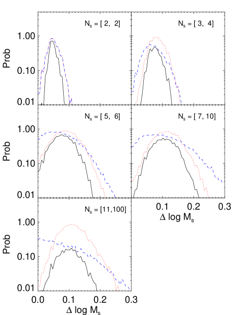
Figure 18.— The KS test probabilities $P_{\rm MGG}$, $P_{\rm SMG}$ and $P_{\rm M,S}$ as function of the average stellar mass increment $\Delta{\rm log}M_{s}$ for 6 different $N_{\rm 19.5}$ bins, which are shown as the dotted, dashed and solid lines respectively in each panel.

As for BGGs, we take the point where the accumulated probability from $\Delta{\rm log}\bar{M}_{s}=0$ is half of the accumulated probability that from $\Delta{\rm log}\bar{M}_{s}=0$ to 0.3 as the best estimation of the $\Delta{\rm log}M_{s}$. The best estimations of the average stellar mass increment($\Delta{\rm log}\bar{M}_{s}$) in logarithm space are [0.05, 0.08, 0.08, 0.10,0.11] dex for five richness bins respectively. The uncertainties of $\Delta{\rm log}\bar{M}_{s}$ are also then calculated from the 68 percentiles of the likelihood distribution on each side. The $\Delta{\rm log}\bar{M}_{s}$ together with their uncertainties are plotted in the top panel of Fig. 7 and are listed in Table 1.

References

- Abazajian (2009) Abazajian, K. N. e. a. 2009, Astrophys. J., 182, 543
- Andreon & Hurn (2010) Andreon, S. & Hurn, M. A. 2010, MNRAS, 404, 1922
- Ascaso et al. (2011) Ascaso, B., Aguerri, J. A. L., Varela, J., Cava, A., Bettoni, D., Moles, M., & D’Onofrio, M. 2011, ApJ, 726, 69
- Becker et al. (2007) Becker, M. R., McKay, T. A., Koester, B., Wechsler, R. H., Rozo, E., Evrard, A., Johnston, D., Sheldon, E., Annis, J., Lau, E., Nichol, R., & Miller, C. 2007, ApJ, 669, 905
- Bell et al. (2003) Bell, E. F., McIntosh, D. H., Katz, N., & Weinberg, M. D. 2003, ApJS, 149, 289
- Bernardi et al. (2007) Bernardi, M., Hyde, J. B., Sheth, R. K., Miller, C. J., & Nichol, R. C. 2007, AJ, 133, 1741
- Bernstein & Bhavsar (2001) Bernstein, J. P. & Bhavsar, S. P. 2001, MNRAS, 322, 625
- Bhavsar (1989) Bhavsar, S. P. 1989, ApJ, 338, 718
- Bhavsar & Barrow (1985) Bhavsar, S. P. & Barrow, J. D. 1985, MNRAS, 213, 857
- Blanton et al. (2005) Blanton, M. R., Schlegel, D. J., Strauss, M. A., Brinkmann, J., Finkbeiner, D., Fukugita, M., Gunn, J. E., Hogg, D. W., Ivezić, Ž., Knapp, G. R., Lupton, R. H., Munn, J. A., Schneider, D. P., Tegmark, M., & Zehavi, I. 2005, AJ, 129, 2562
- Cooray & Milosavljević (2005) Cooray, A. & Milosavljević, M. 2005, ApJ, 627, L85
- Dobos & Csabai (2011) Dobos, L. & Csabai, I. 2011, MNRAS, 414, 1862
- Dubinski (1998) Dubinski, J. 1998, ApJ, 502, 141
- Edwards & Patton (2012) Edwards, L. O. V. & Patton, D. R. 2012, ArXiv e-prints
- Geller & Peebles (1976) Geller, M. J. & Peebles, P. J. E. 1976, ApJ, 206, 939
- Geller & Postman (1983) Geller, M. J. & Postman, M. 1983, ApJ, 274, 31
- Hansen et al. (2005) Hansen, S. M., McKay, T. A., Wechsler, R. H., Annis, J., Sheldon, E. S., & Kimball, A. 2005, ApJ, 633, 122
- Hansen et al. (2009) Hansen, S. M., Sheldon, E. S., Wechsler, R. H., & Koester, B. P. 2009, ApJ, 699, 1333
- Hearin et al. (2013a) Hearin, A. P., Zentner, A. R., Berlind, A. A., & Newman, J. A. 2013a, MNRAS, 433, 659
- Hearin et al. (2013b) Hearin, A. P., Zentner, A. R., Newman, J. A., & Berlind, A. A. 2013b, MNRAS, 430, 1238
- Komatsu et al. (2011) Komatsu, E., Smith, K. M., Dunkley, J., Bennett, C. L., Gold, B., Hinshaw, G., Jarosik, N., Larson, D., Nolta, M. R., Page, L., Spergel, D. N., Halpern, M., Hill, R. S., Kogut, A., Limon, M., Meyer, S. S., Odegard, N., Tucker, G. S., Weiland, J. L., Wollack, E., & Wright, E. L. 2011, ApJS, 192, 18
- Lin et al. (2010) Lin, Y.-T., Ostriker, J. P., & Miller, C. J. 2010, ApJ, 715, 1486
- Liu et al. (2008) Liu, F. S., Xia, X. Y., Mao, S., Wu, H., & Deng, Z. G. 2008, MNRAS, 385, 23
- Loh & Strauss (2006) Loh, Y.-S. & Strauss, M. A. 2006, MNRAS, 366, 373
- More (2012) More, S. 2012, ApJ, 761, 127
- Paranjape & Sheth (2012) Paranjape, A. & Sheth, R. K. 2012, MNRAS, 423, 1845
- Pasquali et al. (2010) Pasquali, A., Gallazzi, A., Fontanot, F., van den Bosch, F. C., De Lucia, G., Mo, H. J., & Yang, X. 2010, MNRAS, 407, 937
- Peebles (1968) Peebles, P. J. E. 1968, ApJ, 153, 13
- Postman & Lauer (1995) Postman, M. & Lauer, T. R. 1995, ApJ, 440, 28
- Rafferty et al. (2008) Rafferty, D. A., McNamara, B. R., & Nulsen, P. E. J. 2008, ApJ, 687, 899
- Rozo et al. (2010) Rozo, E., Wechsler, R. H., Rykoff, E. S., Annis, J. T., Becker, M. R., Evrard, A. E., Frieman, J. A., Hansen, S. M., Hao, J., Johnston, D. E., Koester, B. P., McKay, T. A., Sheldon, E. S., & Weinberg, D. H. 2010, ApJ, 708, 645
- Schlegel et al. (2009) Schlegel, D., White, M., & Eisenstein, D. 2009, in Astronomy, Vol. 2010, astro2010: The Astronomy and Astrophysics Decadal Survey, 314
- Skibba et al. (2011) Skibba, R. A., van den Bosch, F. C., Yang, X., More, S., Mo, H., & Fontanot, F. 2011, MNRAS, 410, 417
- Tal et al. (2012) Tal, T., Wake, D. A., van Dokkum, P. G., van den Bosch, F. C., Schneider, D. P., Brinkmann, J., & Weaver, B. A. 2012, ApJ, 746, 138
- Tavasoli et al. (2011) Tavasoli, S., Khosroshahi, H. G., Koohpaee, A., Rahmani, H., & Ghanbari, J. 2011, PASP, 123, 1
- Tinker et al. (2008) Tinker, J., Kravtsov, A. V., Klypin, A., Abazajian, K., Warren, M., Yepes, G., Gottlöber, S., & Holz, D. E. 2008, ApJ, 688, 709