Critical exponents in Ising Spin Glasses

Abstract

Extensive simulations are made of the spin glass susceptibility and correlation length in five dimension Ising Spin Glasses (ISGs) with Gaussian and bimodal interaction distributions. Once the transition temperature is accurately established using a standard criterion, critical exponents and correction terms can be readily estimated by extrapolating measurements made in the thermodynamic limit regime. The data show that the critical exponents of the susceptibility $\gamma$ and of the correlation length $\nu$ depend on the form of the interaction distribution. This observation implies that quite generally critical exponents are not universal in ISGs.

I Introduction

The universality of critical exponents is an important and remarkably elegant property of standard second order transitions, which has been explored in great detail through the Renormalization Group Theory. The universality hypothesis states that for all systems within a universality class the critical exponents are strictly identical and do not depend on the microscopic parameters of the model. However, universality is not strictly universal; there are known “eccentric”models which violate the universality rule in the sense that their critical exponents vary continuously as a function of a control variable. The most famous example is the eight vertex model solved exactly by Baxter baxter:71 ; there are other scattered cases.

For Ising Spin Glasses (ISGs), the form of the interaction distribution is a microscopic control parameter. It has been assumed that the members of the ISG family of transitions obey standard universality rules, following the generally accepted statement that “Empirically, one finds that all systems in nature belong to one of a comparatively small number of universality classes”stanley:99 .

ISG transition simulations are much more demanding numerically than are those on, say, pure ferromagnet transitions with no interaction disorder. The traditional approach in ISGs has been to study the temperature and size dependence of observables in the near-transition region and to estimate the critical temperature and exponents through finite size scaling relations after taking means over large numbers of samples. Finite size corrections to scaling should be allowed for explicitly which can be delicate. Usually it has been concluded that the numerical data are compatible with universality katzgraber:06 ; hasenbusch:08 ; jorg:08 even though the estimates of the critical exponents have varied considerably from one publication to the next (see Ref. katzgraber:06 for a tabulation of historic estimates).

We have estimated the critical exponents in two ISGs in dimension $5$ using a strategy complementary to the standard finite size scaling method. First we use the Binder cumulant to estimate the critical temperature $\beta_{c}$ reliably and with precision through finite size scaling notebeta . Then using the scaling variable and scaling expressions appropriate for ISGs daboul:04 ; campbell:06 we estimate the temperature dependence of the thermodynamic limit (ThL) ISG susceptibility $\chi(\beta,\infty)$ and second moment correlation length $\xi(\beta,\infty)$ over the entire paramagnetic temperature range from $\beta=0$ to criticality. From these data we estimate the critical exponents and the leading Wegner correction terms wegner:72 . The numerical data show conclusively that for the ISGs in dimension $5$ critical exponents do depend on the form of the interaction distribution. It is relevant that it has been shown experimentally that in Heisenberg spin glasses the critical exponents depend on the strength of the Dzyaloshinski-Moriya interaction campbell:10 .

The Hamiltonian is as usual

$$\mathcal{H}=-\sum_{ij}J_{ij}S_{i}S_{j}$$ (1)

with the near neighbor symmetric bimodal ($\pm J$) or Gaussian distributions normalized to $\langle J_{ij}^{2}\rangle=1$. The Ising spins live on simple [hyper]cubic lattices with periodic boundary conditions.

A natural scaling variable for ISGs with symmetric interaction distributions is $\tau=1-(\beta/\beta_{c})^{2}$ singh:86 ; daboul:04 ; then the standard ThL ISG susceptibility including the leading Wegner correction term wegner:72 is

$$\chi(\beta)=C_{\chi}\tau^{-\gamma}\left(1+a_{\chi}\tau^{\theta}\right)$$ (2)

where $\gamma$ is the critical exponent and $\theta$ the Wegner correction exponent, both of which are characteristic of a university class. As $\chi(\beta=0)=1$, $C_{\chi}=1/(1+a_{\chi})$. Following a protocol well-established for the ferromagnetic case kouvel:64 ; butera:02 one can define a temperature dependent effective exponent $\gamma(\beta)=-\partial\ln\chi(\beta)/\partial\ln\tau$ with $\gamma(\beta)$ tending to the critical $\gamma$ as $\tau\to 0$. A useful exact infinite temperature limit rule from High Temperature Series Expansions (HTSE) for ISGs on simple [hyper]cubic lattices in dimension $d$ daboul:04 is $\gamma(\beta=0)=2d\beta_{c}^{2}$. Samples of size $L$ are in the ThL regime as long as the condition $L>\xi(\beta)$ is satisfied. The exact ThL $\chi(\beta,\infty)$ can be calculated for bimodal and Gaussian ISGs in any dimension using the high temperature series terms tabulated by Daboul et al. daboul:04 over a range of $\beta$ limited by the number of terms ($15$ for bimodal interactions and $13$ for Gaussian) whose values have been explicitly evaluated.

The analogous natural scaling expression for the ISG second moment correlation length $\xi(\beta)$ is campbell:06

$$\xi(\beta)/\beta=C_{\xi}\tau^{-\nu}\left(1+a_{\xi}\tau^{\theta}\right)$$ (3)

or, alternatively, define $\nu(\beta)=-\partial\ln(\xi(\beta)/\beta)/\partial\ln\tau$. The reason for the factor $1/\beta$ is spelt out in Ref. campbell:06 . The $\beta=0$ limit in ISGs in simple [hyper]cubic lattices of dimension $d$ is $\nu(\beta=0)=(d-K/3)\beta_{c}^{2}$ where $K$ is the kurtosis of the interaction distribution.

When samples of finite size $L$ are in the ThL regime, $\chi(L,\beta)$, $\xi(L,\beta)$ and other observables are independent of $L$. Working in the ThL has a number of advantages: the temperatures studied are higher than the critical temperature so equilibration is facilitated, the sample to sample variations are automatically much weaker than at criticality, and there are no finite size scaling corrections to take into account. It can be noted that the particular critical exponent $\eta$ can be estimated without needing $\beta_{c}$ as an input parameter campbell:06 . Otherwise for the temperature dependent effective exponents $\gamma(\tau,L)$ and $\nu(\tau,L)$ it is important to already have an accurate and reliable estimate of $\beta_{c}$ from finite size critical data such as the familiar Binder cumulant or correlation length ratio, or link overlap criteria lundow:13 ; lundow:13a . For the present analysis we have used the critical behavior of the Binder cumulant $g(\beta,L)$ for estimating $\beta_{c}$ as among the dimensionless variables it showed the small finite size corrections for the ISGs studied. Results from the correlation length ratio $\xi(\beta,L)/L$ and link overlap parameters were fully consistent with the Binder estimate. The limit of the ThL regime for each $L$ can be identified by inspection; with $\beta_{c}$ fixed, the envelope curve for the whole set of the ThL regime $\gamma(\tau)$ data points can be extrapolated to $\tau=0$ to obtain an estimate of each of the critical exponents.

A particularly useful method for extending the susceptibility data to criticality is to plot $y=\partial\beta^{2}/\partial\ln\chi(\beta)$ against $x=\beta^{2}$. If correction terms beyond the leading Wegner term can be considered negligible there is an exact expression for the ThL regime:

$$\frac{\partial\beta^{2}}{\ln\chi(\beta)}=\frac{\beta_{c}^{2}\tau(1+a_{\chi}\tau^{\theta})}{\gamma+(\gamma-\theta)a_{\chi}\tau^{\theta}}$$ (4)

The critical intercept $y=0$ occurs when $x=\beta_{c}^{2}$, and the initial slope starting at the intercept is $\partial y/\partial x=-1/\gamma$. If ThL $\chi(\beta,L)$ data to sufficiently large $L$ are available and if the higher order Wegner correction terms are indeed negligible (this should generally be the case except in the region of very small $\beta$) then the four parameters $\beta_{c}^{2},\gamma,\theta$, and $a_{\chi}$ can in principle all be estimated from a single fit to this plot of $\chi(\beta,L)$ data. From the generic form of the HTSE the high temperature $x=0$ intercept is $y=1/2d$ for an ISG in dimension $d$, whatever the interaction distribution and whatever $\beta_{c}$. This reduces the number of free parameters to three, as the condition $a_{\chi}\theta/(a_{\chi}+1)=\gamma-2d\beta_{c}^{2}$ follows. In addition, if $\beta_{c}^{2}$ is already accurately known from independent observations such as finite size scaling, then the precision on the estimates of the other parameters is obviously greatly improved as the fit reduces to a two free parameter interpolation.

There is an analogous expression for $\xi(\beta)/\beta$:

$$\frac{\partial\beta^{2}}{\ln(\xi(\beta)/\beta)}=\frac{\beta_{c}^{2}\tau(1+a_{\xi}\tau^{\theta})}{\nu+(\nu-\theta)a_{\xi}\tau^{\theta}}$$ (5)

with the same $\beta_{c}^{2}$ and $\theta$ as for $\chi(\beta)$. The $y=0$ intercept is again $x=\beta_{c}^{2}$, with an initial slope at the intercept equal to $\partial y/\partial x=-1/\nu$. The $x=0$ intercept is $y=3/(3d-K)$, where again $d$ is the dimension and $K$ the interaction distribution kurtosis. Then, by analogy with Eq. (4), the condition $a_{\xi}\theta/(a_{\xi}+1)=\nu-((3d-K)/3)\beta_{c}^{2}$ holds, so $\nu$ is the only remaining free parameter in the Eq. (5) fit.

The simulations were carried out using exchange Monte Carlo on $256$ samples at each size. Error bars on the finite difference derivatives in Eqs. (4) and  (5) are from the bootstrap method, though it is clear that for a finite difference derivative such estimates are not very meaningful.

For the $5$d Gaussian ISG the HTSE critical temperature and exponent estimates are daboul:04 $\beta_{c}=0.4207(35)$ and $\gamma=1.75(15)$. From the intersections of the present $g(\beta,L)$ curves $\beta_{c}=0.419(1)$, see Fig. 1. No finite size correction for the Binder cumulant is visible, so the $\beta_{c}$ estimate is particularly reliable. There is full agreement between the $\beta_{c}$ estimate from $g(\beta,L)$ and the HTSE central value, with the former being considerably more accurate. With $\beta_{c}^{2}$ fixed at $0.419^{2}=0.1755$, the optimal interpolation fit to the HTSE and simulation ISG susceptibility data using Eq. (4), Fig. 2, is with parameters $\gamma=1.62(3),\theta=3.0(5)$, and $a_{\chi}=-0.0445(50)$. These values are the best fit estimates and the error bars allow for the residual uncertainty in $\beta_{c}$. The final tabulated HTSE $\gamma$ estimate in daboul:04 appears to be in only marginal agreement with the present estimate. However, it can be noted that each individual HTSE Dlog Padé $\beta_{c}^{2}$ estimate is accompanied by a $\gamma$ estimate in almost perfect one-to-one correspondence, see Fig. 7 of Ref. daboul:04 . Reading off this figure, if $\beta_{c}^{2}=0.1755$, then $\gamma\sim 1.61$. Hence there is excellent agreement between the present $\gamma$ estimate and the HTSE Dlog Padé estimates. The present high $\theta$ and low $a_{\chi}$ estimates show that Wegner correction is weak and the residual leading correction term is of high order. This may explain why estimates from the M1 and M2 HTSE protocols daboul:04 are different from the Dlog Padé estimates in this particular case.

The correlation length $\xi(\beta,L)$ simulation data were analysed following just the same procedure using Eq. (5), with $\beta_{c}^{2}$ and $\theta$ held fixed at the same values as estimated above. Unfortunately there are no HTSE results available except for the $\beta^{2}=0$ limit point. The $\xi(\beta,L)$ simulation data are intrinsically more noisy than the $\chi(\beta,L)$ data. The optimal fit to the $\partial\beta^{2}/\partial\ln(T\xi(\beta))$ data plot for the Gaussian interactions, Fig. 3, with the same $\beta_{c}^{2}$ and $\theta$ gave the estimate $\nu=0.71(2)$ and $a_{\xi}=0.004(2)$ (or $C_{\xi}\sim 1.00$). The Wegner correction term is tiny. From the general scaling rule $\gamma=(2-\eta)\nu$, we can estimate $\eta=-0.28(4)$.

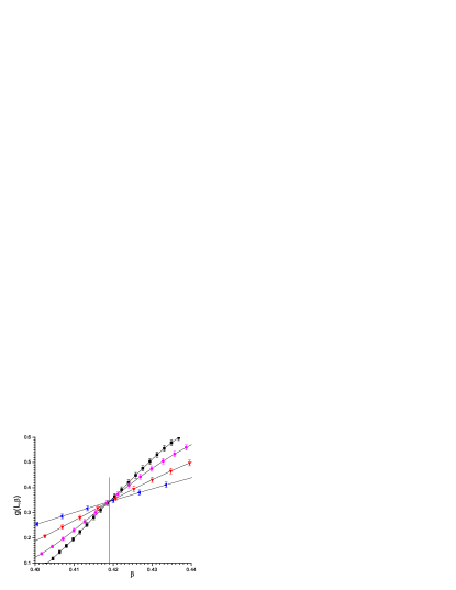
Figure 1: (Color online) The Binder cumulant $g(\beta,L)$ for even $L$ $5$d Gaussian interaction samples; symbol coding: black squares $L=10$, pink circles $L=8$, red inverted triangles $L=6$, blue left triangles $L=4$. The vertical red line corresponds to $\beta_{c}=0.419$.

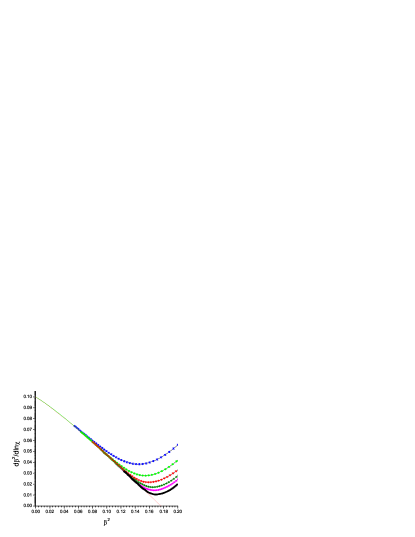
Figure 2: (Color online) $\partial\beta^{2}/\partial\ln\chi(\beta)$ for $5$d Gaussian interaction samples. Symbol coding as in Fig. 1 plus olive triangle $L=7$, green diamond $L=5$. The full green curve calculated directly from HTSE continues to represent the ThL $\chi(\beta)$ up to $\beta^{2}\sim 0.13$. Dashed red curve: fit Eq. (4). The overall ThL envelope can be seen by inspection.

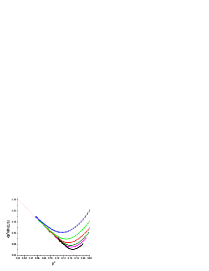
Figure 3: (Color online) $\partial\beta^{2}/\partial\ln(\xi(\beta)/\beta)$ for $5$d Gaussian interaction samples. Symbol coding as in Fig. 2.

For the $5$d bimodal ISG the HTSE critical temperature estimate daboul:04 is $\beta_{c}=0.3925(40)$. From the intersections of the $g(\beta,L)$ curves $\beta_{c}=0.3925(10)$, Fig. 4. The finite size $g(\beta,L)$ corrections are stronger than in the Gaussian case. There is full agreement between the Binder cumulant $\beta_{c}$ estimate and the central value of the HTSE $\beta_{c}$ estimate, with the former error bars being considerably smaller than the HTSE error bars. With $\beta_{c}^{2}$ fixed at $0.3925^{2}=0.1540$, the optimal interpolation fit to the HTSE and simulation ISG susceptibility data using Eq. (4), Fig. 4, is with fit parameters $\gamma=1.99(4),\theta=0.88(5)$, and $a_{\chi}=0.89$ (so $C_{\chi}=0.53$). These values are the best fit estimates and the error bars allow for the residual uncertainty in $\beta_{c}$. The agreement with the central HTSE estimate $\gamma=1.95(15)$ is excellent but the errors on the present value are much smaller because the estimate is based on information from both HTSE and from simulations. The same data can be plotted as $\gamma(\tau)$ against $\tau$ up to $\tau=0$ where a consistent estimate of $\gamma$ is obtained, or as $\chi(\tau)\tau^{\gamma}$ against $\tau^{\theta}$, where the ThL regime data indeed fall on a straight line with intercept $C_{\chi}=1/(1+a_{\chi})$ confirming that the higher order Wegner corrections are negligible. It can be noted that the HTSE analysis daboul:04 provided only a rough estimate $\theta\sim 1.0$; no indication of the sign or value of the important correction term strength parameter $a_{\chi}$ was given.

Figure 4: (Color online) The Binder cumulant $g(\beta,L)$ for $5$d bimodal interaction samples with color coding as in Fig 1. The vertical red line corresponds to $\beta_{c}=0.3925$.

Figure 5: (Color online) $\partial\beta^{2}/\partial\ln\chi(\beta)$ for $5$d bimodal interaction samples. Symbol coding as in Fig. 2. Continuous green curve calculated from the exact terms in the HTSE ISG susceptibility tabulation daboul:04 (continues up to $\beta^{2}\sim 0.10$). Dashed red curve : fit Eq. (4).

The correlation length $\xi(\beta,L)$ simulation data were analysed using Eq. (5). The optimal fit was with $\nu=0.86(2)$ and $a_{\xi}=0.19$ (or $C_{\xi}=0.84$). The analogous alternative plots were made for $\xi(\beta,L)$ as for $\chi(\beta,L)$, and again full consistency was observed. The estimate $\eta=-0.32(4)$ follows from the scaling rule $\gamma=\nu(2-\eta)$.

II Conclusions

In conclusion, numerical information on finite size scaling observables, on the ISG susceptibility and on the correlation length from simulations has been combined with information from the exact 15 (bimodal) or 13 (Gaussian) term HTSE susceptibility tables daboul:04 to obtain high precision empirical estimates of the critical temperatures $\beta_{c}$, the critical exponents $\gamma$ and $\nu$, and the parameters of the leading Wegner correction terms, for the bimodal and Gaussian ISGs in dimension $5$. The $\beta_{c}$ values are in full agreement with, but are considerably more precise than, estimates from HTSE alone daboul:04 . As a result and because of the use of a novel analysis protocol for the ThL data, the precision on the $\gamma$ estimates is improved by a factor of the order of $5$ as compared with the estimates obtained in Ref. daboul:04 . The present $\nu$ estimates are of similar quality to those for $\gamma$; there are no published $\nu$ values in dimension $5$ to compare with.

The accurate estimates of $\gamma$ and $\nu$ show that the bimodal and Gaussian ISGs in $5$d have different critical exponents. Results in dimension $4$ lundow:13a and a reanalysis of data in dimension $3$ taking special care concerning the estimates of the critical temperatures lundow confirm this conclusion. These results clearly imply that in the entire family of ISGs the critical exponents are dependent on the form of the interaction distribution, a “microscopic”parameter. Other model parameters, such as a bias in the interaction distribution, could be explored. It would obviously be of fundamental interest to understand the basic origin of this lack of universality at ISG transitions.

III Acknowledgements

We are very grateful to K. Hukushima for comments and communication of unpublished data. We thank Amnon Aharony for constructive criticism. The computations were performed on resources provided by the Swedish National Infrastructure for Computing (SNIC) at the High Performance Computing Center North (HPC2N).

References

- (1) R. Baxter, Phys. Rev. Lett. 26, 832 (1971)
- (2) H. E. Stanley, Rev. Mod. Phys. 71, S358 (1999)
- (3) H. G. Katzgraber, M. Korner, and A. P. Young, Phys. Rev. B 73, 224432 (2006).
- (4) M. Hasenbusch, A. Pelissetto, and E. Vicari, Phys. Rev. B 78, 214205 (2008).
- (5) T. Jörg and H. G. Katzgraber, Phys. Rev. B 77, 214426 (2008).
- (6) We will use inverse temperatures throughout.
- (7) D. Daboul, I. Chang and A. Aharony, Eur. Phys. J. B 41, 231 (2004).
- (8) I. A. Campbell, K. Hukushima, and H. Takayama, Phys. Rev. Lett. 97, 117202 (2006).
- (9) F. Wegner, Phys. Rev. B 5, 4529 (1972).
- (10) I. A. Campbell and D. C. M. C. Petit, J. Phys. Soc. Japan, 79, 011006 (2010)
- (11) R. R. P. Singh and S. Chakravarty, Phys. Rev. Lett. 57, 245 (1986).
- (12) J. Kouvel and M. E. Fisher, Phys. Rev. A 136, 1626 (1964).
- (13) P. Butera and M. Comi, Phys. Rev. B 65,144431 (2002).
- (14) P. H. Lundow and I. A. Campbell, Phys. Rev. E 87, 022102 (2013)
- (15) P. H. Lundow and I. A. Campbell, arXiv:1302.1100
- (16) P. H. Lundow and I. A. Campbell, unpublished.